Generalized dynamical equation and low energy nucleon dynamics

Abstract

Low energy nucleon dynamics is investigated by using the generalized dynamical equation derived in [J. Phys. A v.32, 5657 (1999)]. This equation extends quantum dynamics to describe the time evolution in the case of nonlocal-in-time interactions. We show that the use of the generalized dynamical equation, which allows one to take into account that effective actions in quantum field theory, arising after integrating out certain degrees of freedom, are generally nonlocal, provides a new way to formulate the effective theory of nuclear forces. In this way we construct the most general possible operator describing the short-range part of the $NN$ interaction in the ${}^{1}S_{0}$ channel. In particular, this operator can be incorporated into the chiral potential model. This is shown to provide an extension of the standard chiral approach. Being equivalent to the chiral potential model for some values of the constants characterizing the short-range of the $NN$ interaction this approach allows the solutions that cannot be reproduced by any potential model. In this way we find that for certain values of the constants inconsistent with potentials models the effect of the short-range forces on the half off-shell $2N$ $T$-matrix with high off-shell momenta grows in magnitude rapidly as the kinetic energy of outgoing protons decreases at laboratory energies below $15$ $MeV$. We show that this effect may be the origin of the existing discrepancy between the theory and experiment in describing the proton-proton bremsstrahlung.

I Introduction

Ideas from the foundations of quantum mechanics are being applied now to many branches of physics. In the quantum mechanics of particles interacting through the Coulomb potential one deals with a well-defined interaction Hamiltonian and the Schrödinger equation governing the dynamics of the theory. This theory is perfectly consistent and provides an excellent description of atomic phenomena at low energies. It is natural to expect that low energy nuclear physics can be described in the same way. However, one has not yet constructed a fundamental nucleon-nucleon (NN) potential. Nowadays there exist phenomenological $NN$ potentials which successfully describe scattering data to high precision, but they do not emerge from QCD and contain $ad$ $hoc$ form factors. A first attempt to systematically solve the problem of low energy nucleon dynamics and construct a bridge to QCD was made by Weinberg EFT3 . He suggested to derive a $NN$ potential in time-ordered chiral perturbation theory (ChPT). However, such a potential is singular and the Schrödinger (Lippmann-Schwinger) equation does not make sense without regularization and renormalization. This means that in the effective field theory (EFT) of nuclear forces, which following the pioneering work of Weinberg has become very popular in nuclear physics (for a review, see Ref. rev ), the Schrödinger equation is not valid. On the other hand, the whole formalism of fields and particles can be considered as an inevitable consequence of quantum mechanics, Lorentz invariance, and the cluster decomposition principle Weinberg97 . Thus in the nonrelativistic limit QCD must reproduce low energy nucleon physics consistent with the basic principles of quantum mechanics. However, as it follows from the Weinberg analysis, QCD leads through ChPT to the low energy theory in which the Schrödinger equation is not valid. This means that either there is something wrong with QCD and ChPT or the Schrödinger equation is not the basic dynamical equation of quantum theory. Meanwhile, in Ref. R.Kh.:1999 it has been shown that the Schrödinger equation is not the most general equation consistent with the current concepts of quantum physics, and a more general equation of motion has been derived as a consequence of the basic postulates of the Feynman Feynman:1948 and canonical approaches to quantum theory. Being equivalent to the Schrödinger equation in the case of instantaneous interactions, this generalized dynamical equation permits the generalization to the case where the dynamics of a system is generated by a nonlocal-in-time interaction. The generalized quantum dynamics (GQD) developed in this way has proved an useful tool for solving various problems in quantum theory PRC:2002 ; PLA:2002 .

The GQD allows one to consider the problem of consistency of quantum mechanics with the low energy predictions of QCD from a new point of view. From this viewpoint, in investigating the consequences of ChPT we must not restrict ourselves to the assumption that the $NN$ interaction can be parametrized by a $NN$ potential, and low energy nucleon dynamics is governed by the Schrödinger equation. This dynamics may be governed by the generalized dynamical equation (GDE) with a nonlocal-in-time interaction operator when this equation is not equivalent to the Schrödinger equation, and hence the above divergence problems may be the cost of trying to describe low energy nucleon dynamics in terms of Hamiltonian formalism while this dynamics is really non-Hamiltonian. Another motivation for investigating the problem of the description of nucleon dynamics from the point of view of the formalism of the GQD is still existing discrepancy between the predictions of the modern $NN$ potential models and experiment. For example, there is a significant discrepancy between theory and experiment in describing the proton-proton ($pp$) bremsstrahlung M-S that is an accurate test of $NN$ interaction models. An important part of this discrepancy originates in a poor description of the $NN$ interaction at low energies C-T . The formalism of the GQD that reproduces the potential models of the $NN$ interaction in the particular case when this interaction is assumed to be instantaneous admits a more general class of such models, and only experiment such as the $pp$ bremsstrahlung can discriminate between them. In this context the discrepancy between the predictions of the potential models and experiment should mean that in describing nucleon dynamics one cannot ignore that the $NN$ interaction is nonlocal in time.

The aim of the present paper is twofold. From the one hand, we intend to show that the low energy predictions of QCD are consistent with the basic principles of quantum mechanics, but in this case a new insight into these principles provided by the formalism of the GQD is needed. On the other hand, it is our intention to demonstrate that this formalism allows one to formulate the effective theory of nuclear forces as an inevitable consequence of the basic principles of quantum mechanics and the symmetries of QCD. Being formulated in this way the theory of nuclear forces opens new possibilities for describing nucleon dynamics at low energies. In Sec. II we briefly consider the main features of the formalism of the GQD developed by one of the authors (R.G.) in Ref. R.Kh.:1999 . We mainly focus on the physical meaning of the GDE which is a direct consequence of the principle of the superposition of the probability amplitudes and the requirement that the evolution operator is unitary. This equation plays a key role in the present work.

In Sec. III we consider the pionless theory of nuclear forces. By focusing the attention on the ${}^{1}S_{0}$ channel, we show that the requirement that the two-nucleon $(2N)$ $T$-matrix satisfies the GDE and is consistent with the symmetries of QCD allows one to construct this $T$-matrix by expanding it in powers of $Q/\Lambda$ where $Q$ being some low energy scale, and $\Lambda$ is the scale at which the theory is expected to break down. In this way we can reproduce all results for the $NN$ scattering amplitudes obtained in the standard EFT of nuclear forces. It is important that these results are reproduced starting with a well defined $2N$ $T$-matrix without resorting to the regularization and renormalization procedures. In Sec. IV we show that the use of the GDE allows one to formulate the effective theory as a perfectly consistent theory free from UV divergences. Being formulated in this way, the effective theory keeps all advantages of the traditional nuclear physics approach. At the same time, its advantage over the traditional approach is that it allows one to find constraints on the off-shell behavior of the $2N$ $T$-matrix that are placed by the symmetries of QCD.

In Sec. V the proposed formalism is considered from the point of view of the Weinberg program for physics of the two-nucleon systems. The approach based on the derivation of a $NN$ potential from ChPT was pioneered by Weinberg Weinberg97 and developed by Ordônez Ordonez and van Kolck van Kolck . Recently the potential at fourth order of ChPT that reproduce the $NN$ data with the same accuracy as phenomenological high-precision potentials was developed by Entem and Machleidt Entem2 . We show that our formulation of the effective theory of nuclear forces is a generalization of the above approach. Instead of the Schrödinger (LS) equation, it is suggested to use the GDE. In this way we construct the most general possible operator describing the short-range part of the $NN$ interaction. We show that this operator can be incorporated into the chiral approach. Being equivalent to the chiral potential model for some values of the constants characterizing the short-range part of the $NN$ interaction this approach allows the solutions that cannot be reproduced by any potential model. In Sec. VI we show that the for certain values of the constants inconsistent with potentials models the effect of the short-range forces on the $2N$ $T$-matrix with high off-shell momenta grows in magnitude rapidly as the kinetic energy of outgoing protons decreases in the region below $15$ $MeV$. We also show that the fact that the existing microscopic $pp$ bremsstrahlung models cannot reproduce this effect may be the origin of the discrepancy between their predictions and the experimental data. We also show that our formalism allows one to modify the short-range parts of the existing high-precision potentials to improve their off-shell predictions keeping the phase shifts unchanged. New possibilities that the formalism of the GQD opens for solving three-body problem in nuclear physics are discussed in Sec. VII.

II Generalized quantum dynamics

The basic concept of the canonical formalism of quantum theory is that it can be formulated in terms of vectors of a Hilbert space and operators acting on this space. In this formalism the postulates that establish the connection between the vectors and operators and states of a quantum system and observables are used together with the dynamical postulate according to which the time evolution of a quantum system is governed by the Schrödinger equation. In the Feynman formalism quantum theory is formulated in terms of probability amplitudes without resorting to vectors and operators acting on a Hilbert space. Feynman’s theory starts with an analysis of the phenomenon of quantum interference. The results of this analysis which leads directly to the concept of the superposition of probability amplitudes are summarized by the following postulate Feynman:1948 :

The probability of an event is the absolute square of a complex number called the probability amplitude. The joint probability amplitude of a time-ordered sequence of events is the product of separate probability amplitudes of each of these events. The probability amplitude of an event which can happen in several different ways is a sum of the probability amplitudes for each of these ways.

The Feynman formulation is based on the assumption that the history of a quantum system can be represented by some path in space-time, and hence the probability amplitude of any event is a sum of the probability amplitudes that a particle has a completely specified path in space-time. The contribution from a single path is postulated to be an exponential whose (imaginary) phase is the classical action (in units of $\hbar$) for the path in question. This assumption is not as fundamental as the above principle of the superposition of probability amplitudes which follows directly from the analyzes of the phenomenon of quantum interference. This fact is emphasized, for example, in Feynman’s book Feyn , where a minimal set of physical principles which must be satisfied in any theory of fields and particles is analyzed. Feynman includes in this set neither the second postulate of his formalism nor the Schrödinger equation: The only quantum mechanical principle included in this set is the principle of the superposition of probability amplitudes. In Ref. R.Kh.:1999 it has been shown that, instead of processes associated with a completely specified path in space-time, one can use processes associated with completely specified instants of the beginning and end of interaction in a quantum system as alternative ways in which any event can happen. As it turned out, employing this class of alternatives allows one to derive a dynamical equation from the principle of the superposition without making supplementary assumptions like the second postulate of Feynman’s theory. By using this class of alternatives and the superposition principle, $\langle\psi|U(t,t_{0})|\varphi\rangle$, being the probability amplitude of finding a quantum system in the state $|\psi\rangle$ in a measurement at time $t$, if at time $t_{0}$ it was in the state $|\varphi\rangle$, can be represented in the form R.Kh.:1999

$$\langle\psi|U(t,t_{0})|\varphi\rangle=\langle\psi|\varphi\rangle+\int_{t_{0}}^{t}dt_{2}\int_{t_{0}}^{t_{2}}dt_{1}\langle\psi|\tilde{S}(t_{2},t_{1})|\varphi\rangle.$$ (1)

Here $\langle\psi|\tilde{S}(t_{2},t_{1})|\varphi\rangle$ is the probability amplitude that, if at time $t_{1}$ the system was in the state $|\varphi\rangle,$ then the interaction in the system will begin at time $t_{1}$ and end at time $t_{2}$ and at this time the system will be in the state $|\psi\rangle.$ By using the operator formalism, one can represent amplitudes $\langle\psi|U(t,t_{0})|\varphi\rangle$ by the matrix elements of the unitary evolution operator $U(t,t_{0})$ in the interaction picture. The operator $\tilde{S}(t_{2},t_{1})$ represents the contribution to the evolution operator from the process in which the interaction in the system begins at time $t_{1}$ and ends at time $t_{2}$. As has been shown in Ref. R.Kh.:1999 , for the evolution operator (1) to be unitary for any $t$ and $t_{0}$ the operator $\tilde{S}(t_{2},t_{1})$ must satisfy the equation

$$(t_{2}-t_{1})\tilde{S}(t_{2},t_{1})$$ (2)

$$= \int^{t_{2}}_{t_{1}}dt_{4}\int^{t_{4}}_{t_{1}}dt_{3}(t_{4}-t_{3})\tilde{S}(t_{2},t_{4})\tilde{S}(t_{3},t_{1}).$$

A remarkable feature of this equation is that it works as a recursion relation and allows one to obtain the operators $\tilde{S}(t_{2},t_{1})$ for any $t_{1}$ and $t_{2}$, if $\tilde{S}(t^{\prime}_{2},t^{\prime}_{1})$ corresponding to infinitesimal duration times $\tau=t^{\prime}_{2}-t^{\prime}_{1}$ of interaction are known. It is natural to assume that most of the contribution to the evolution operator in the limit $t_{2}\to t_{1}$ comes from the processes associated with the fundamental interaction in the system under study. Denoting this contribution by $H_{int}(t_{2},t_{1})$ we can write

$$\tilde{S}(t_{2},t_{1})\mathop{\to}\limits_{t_{2}\rightarrow t_{1}}H_{int}(t_{2},t_{1})+o(\tau^{\epsilon}),$$ (3)

where $\tau=t_{2}-t_{1}$. The parameter $\varepsilon$ is determined by demanding that $H_{int}(t_{2},t_{1})$ called the generalized interaction operator must be so close to the solution of Eq. (2) in the limit $t_{2}\mathop{\to}t_{1}$ that this equation has a unique solution having the behavior (3) near the point $t_{2}=t_{1}$. If $H_{int}(t_{2},t_{1})$ is specified, Eq. (2) allows one to find the operator $\tilde{S}(t_{2},t_{1})$, and hence the evolution operator. Thus Eq. (2) can be regarded as an equation of motion for states of a quantum system. This generalized dynamical equation allows one to construct the evolution operator by using the contributions from fundamental processes as building blocks. In the case of Hamiltonian dynamics the fundamental interaction is instantaneous. The generalized interaction operator describing such an interaction is of the form

$$H_{int}(t_{2},t_{1})=-2i\delta(t_{2}-t_{1})H_{I}(t_{1})$$ (4)

(the delta function $\delta(t_{2}-t_{1})$ emphasizes that the interaction is instantaneous). In this case Eq. (2) is equivalent to the Schrödinger equation R.Kh.:1999 with the operator $H_{I}(t)$ being an interaction Hamiltonian (in the interaction picture). At the same time, Eq. (2) permits the generalization to the case where the fundamental interaction in a quantum system is nonlocal in time, and hence the dynamics is non-Hamiltonian R.Kh.:1999 .

Let us now briefly consider (for details see Ref. R.Kh.:1999 ) the mathematical assumptions on which the formalism of the GQD is founded. As we already noted, in the canonical formalism the assumption that the evolution of a quantum system is governed by the Schrödinger equation is used as a dynamical postulate. On the other hand, since the operator $V(t)\equiv U(t,0)$ is postulated to be unitary with the group properties

$$V(t_{2},t_{1})=V(t_{2})V(t_{1}),\quad V(0)=1,$$

from Stone’s theorem it follows that, if this one-parameter group is weekly continuous, i.e.,

$$\langle\psi_{2}|V(t_{2})|\psi_{1}\rangle\mathop{\to}\limits_{t_{2}\to t_{1}}\langle\psi_{2}|V(t_{1})|\psi_{1}\rangle$$ (5)

for any $|\psi_{1}\rangle$ and $|\psi_{2}\rangle$ belonging to the Hilbert space, than it has a self-adjoint infinitesimal generator $H$:

$$V(t)=\exp(-iHt),\quad idV(t)/dt=HV(t).$$

Identifying $H$ with the total Hamiltonian as usual, we get the Schrödinger equation. Thus the assumption that this equation governs the dynamics of a system is equivalent to the assumption that the evolution operator satisfies the condition (5). However, from the physical point of view, Eq. (5) must not be satisfied for any states belonging to the Hilbert space. In fact, there are normalized vectors in the Hilbert space that represent the states for which energy of a system is infinite. From the point of view of the states with infinite energy $|\psi_{in}\rangle$ any time interval $\delta t$ is infinite, and hence the evolution operator $U(\delta t,0)\equiv 1+R(\delta t,0)$ must be independent of $\delta t$, i.e., must be constant

$$\langle\psi^{\prime}_{in}|U(\delta t,0)|\psi_{in}\rangle=\langle\psi^{\prime}_{in}|\psi_{in}\rangle+\langle\psi^{\prime}_{in}|R(\infty,0)|\psi_{in}\rangle.$$

This means that for the evolution operator to be weekly continuous, $\langle\psi^{\prime}_{in}|R(\infty,0)|\psi_{in}\rangle$ must be zero. However, in quantum field theory, for example, this is not the case because in this theory renormalization is necessary to effectively cut off intermediate states with infinite energy. On the other hand, the states $|\psi_{in}\rangle$ are not physically realizable, and hence from the physical point of view it is enough to require that the condition (5) must be satisfied only for the physically realizable states. The main idea of the formalism of the GQD is that in describing the dynamics of a system one need not to restrict oneself to the assumption that the evolution operator is necessarily weekly continuous, and therefore dynamics is necessarily governed by the Schrödinger equation. In Ref. R.Kh.:1999 it has been shown that the current concepts of quantum physics generate the dynamical principle in which the above assumption does not play any role. In this way the GDE has been derived as the most general dynamical equation. This equation allows one to construct the evolution operator starting with the contributions from the processes with infinitesimal duration times of interaction that are described by the interaction operator $H_{int}(t_{2},t_{1})$, while the Schrödinger equation constructs the evolution operator starting with the contributions from the processes with instantaneous interaction that are described by the interaction Hamiltonian. The GDE allows one to describe, in a consistent way, the dynamics of a quantum system with a nonlocal in time interaction. This equation is equivalent to the Schrödinger equation in the case when the interaction in a system is instantaneous. In the case of nonlocal-in-time interactions the dynamics is determined by the behavior of the interaction operator $H_{int}(t_{2},t_{1})$ in the infinitesimal neighborhood of the point $t_{2}=t_{1}$, i.e., such a nonlocality has no a definite scale. This scale should depend on the problem we consider: Some duration time of interaction may seem as infinitesimal from the point of view of low energy physics, but at the same time it may seem as finite from viewpoint of high energy physics. Thus the GDE allows one to take into account, in a consistent way, that every theory with which we deal is a low energy approximation to a more fundamental one and provides a bridge between them. This is may be important for describing the dynamics in the effective theory of nuclear forces. In this case the duration times of interaction much above the time scale of low energy nuclear physics but much below the scale at which high energy degrees of freedom come into play should be considered as ”infinitesimal”, and the operator describing the processes with such duration times of interaction can be used as an effective interaction operator.

By using Eq. (1), for $U(t,t_{0})$, we can write

$$U(t,t_{0}) = {\bf 1}+\frac{i}{2\pi}\int^{\infty}_{-\infty}dx\exp[-i(z-H_{0})t]$$

$$\times (z-H_{0})^{-1}T(z)(z-H_{0})^{-1}\exp[i(z-H_{0})t_{0}],$$

where $z=x+iy$, $y>0$, and $H_{0}$ is the free Hamiltonian. The operator $T(z)$ is defined by

$$T(z)=i\int_{0}^{\infty}d\tau\exp(iz\tau)\tilde{T}(\tau),$$ (7)

where $\tilde{T}(\tau)=\exp(-iH_{0}t_{2})\tilde{S}(t_{2},t_{1})\exp(iH_{0}t_{1})$, and $\tau=t_{2}-t_{1}$. In terms of the $T$-matrix defined by Eq. (7) the equation of motion (2) can be rewritten in the form R.Kh.:1999

$$\frac{d\langle\psi_{2}|T(z)|\psi_{1}\rangle}{dz}=-\sum\limits_{n}\frac{\langle\psi_{2}|T(z)|n\rangle\langle n|T(z)|\psi_{1}\rangle}{(z-E_{n})^{2}},$$ (8)

where $n$ stands for the entire set of discrete and continuous variables that characterize the system in full, and $|n\rangle$ are the eigenvectors of $H_{0}$. As it follows from Eqs. (3) and (7), the boundary condition on this equation is of the form

$$\langle\psi_{2}|T(z)|\psi_{1}\rangle\mathop{\to}\limits_{|z|\mathop{\to}\infty}\langle\psi_{2}|B(z)|\psi_{1}\rangle+o\left(|z|^{-\beta}\right)$$

$$=\langle\psi_{2}|B(z)|\psi_{1}\rangle+O\left\{h(z)\right\},$$ (9)

$$B(z)=i\int_{0}^{\infty}d\tau\exp(iz\tau)H_{int}^{(s)}(\tau),$$ (10)

where

$$H^{(s)}_{int}(t_{2}-t_{1})=\exp(-iH_{0}t_{2})H_{int}(t_{2},t_{1})\exp(iH_{0}t_{1})$$

is the interaction operator in the Schrödinger picture, and $h(z)$ is an arbitrary function satisfying the condition $h(z)=o\left(|z|^{-\beta}\right)$, $|z|\to\infty$, with $\beta=\varepsilon+1$. In the case of the Hamiltonian dynamics when $H_{int}^{(s)}(\tau)=-2i\delta(\tau)H_{I}$, with $H_{I}$ being the interaction Hamiltonian in the Schrödinger picture, $B(z)=H_{I}$, and the boundary condition (9) takes the form

$$T(z)\mathop{\to}\limits_{|z|\mathop{\to}\infty}H_{I}.$$ (11)

Equation (8) with this boundary condition is equivalent to the Lippmann-Schwinger (LS) equation with the interaction Hamiltonian $H_{I}$. By definition, the operator $B(z)$ is the interaction operator in the energy representation. This operator must be so close to the relevant solution of Eq. (8) in the limit $|z|\to\infty$ that this differential equation has a unique solution having the asymptotic behavior (9). For this the operator $B(z)$ must satisfy the condition

$$\frac{d\langle\psi_{2}|B(z)|\psi_{1}\rangle}{dz} = -\sum\limits_{n}\frac{\langle\psi_{2}|B(z)|n\rangle\langle n|B(z)|\psi_{1}\rangle}{(z-E_{n})^{2}}$$ (12)

$$+ o(|z|^{-\beta-1}),\qquad|z|\to\infty.$$

From Eq. (II) it follows that the evolution operator in the Schrödinger picture can be represented in the form

$$U_{s}(t,0)=\frac{i}{2\pi}\int\limits_{-\infty}^{\infty}dx\exp(-izt)G(z),$$ (13)

where $z=x+iy$, $y>0$, and

$$G(z)=G_{0}(z)+G_{0}(z)T(z)G_{0}(z)$$ (14)

with $G_{0}(z)=\frac{1}{z-H_{0}}.$ Being equivalent to representation (1), Eqs. (13) and (14) express the principle of the superposition of probability amplitudes. In the ordinary quantum mechanics the similar equation plays an important role and establishes the connection between the evolution operator and the Green operator $G(z)$ which is defined by

$$G(z)=\frac{1}{z-H},$$ (15)

with $H$ being the total Hamiltonian. Such a form of the Green operator follows from the fact that in the Hamiltonian formalism the evolution operator satisfies the Schrödinger equation. In the canonical formalism the $T$-matrix is defined by Eq. (14) starting with the Green operator of the form (15). In the formalism of the GQD the $T$-matrix plays a more fundamental role. It is defined by Eq. (7), and in this case the starting point is representation (1) with $\tilde{S}(t_{2},t_{1})$ being the contribution to the evolution operator from the processes in which the interaction begins at time $t_{1}$ and ends at time $t_{2}$. In this case the operator $G(z)$ itself is defined by Eq. (14) via the $T$-matrix. This is a more general definition of the Green operator, since representation (1) is a consequence of the principle of the superposition of probability amplitudes and must be valid in any case while the evolution operator can be represented in the form (13) with the operator $G(z)$ given by Eq. (15) only in the case where the interaction in a system is instantaneous.

As has been shown in Ref. PRC:2002 , there is a one-to-one correspondence between the character of the dynamics and the large-momentum behavior of the $T$-matrix. If this behavior satisfies the requirements of ordinary quantum mechanics, then the interaction in a system is instantaneous and the dynamics is Hamiltonian. In the case where this behavior is ”bad”, i.e., does not meet the requirements of the ordinary quantum mechanics, the interaction generating the dynamics of the system must necessarily be nonlocal-in-time. Let us now illustrate this point by using the model developed in Refs. R.Kh.:1999 ; PRC:2002 as a test model demonstrating the possibility of the extension of quantum dynamics provided by the GQD. This model describes the evolution of the system of two identical nonrelativistic particles with the mass $m$ whose interaction is separable, and hence the interaction operator has the form

$$<{\bf p}_{2}|H_{int}^{(s)}(\tau)|{\bf p}_{1}>=\varphi^{*}({\bf p}_{2})\varphi({\bf p}_{1})f(\tau),$$

where ${\bf p}$ is the relative momentum of the particles, and $f(\tau)$ is some function of the duration time $\tau$ of the interaction in the system. It is assumed that in the limit $|{\bf p}|\to\infty$ the form factor $\varphi({\bf p})$ behave as

$$\varphi({\bf p})\sim|{\bf p}|^{-\alpha},\quad{(|{\bf p}|\mathop{\to}\infty).}$$

In this case the general solution of Eq. (8) is PRC:2002

$$\langle{\bf p}_{2}|T(z)|{\bf p}_{1}\rangle=\frac{\varphi^{*}({\bf p}_{2})\varphi({\bf p}_{1})}{g_{a}^{-1}+(z-a)\int\frac{d^{3}k}{(2\pi)^{3}}\frac{|\varphi({\bf k})|^{2}}{(z-E_{k})(a-E_{k})}},$$ (16)

where $g_{a}=t(a)$, and $a\in(-\infty,0]$. In the case $\alpha>\frac{1}{2}$, the amplitude $\langle{\bf p_{2}}|T(z)|{\bf p_{1}}\rangle$ given by Eq. (16), tends to $\lambda\varphi^{*}({\bf p}_{2})\varphi({\bf p}_{1})$, where

$$\lambda=\left(g_{a}^{-1}+\int\frac{d^{3}k}{(2\pi)^{3}}\frac{|\varphi({\bf k})|^{2}}{a-E_{k}}\right)^{-1}.$$

From Eqs. (9) and (10) it follows that in this case the interaction operator $H_{int}^{(s)}(\tau)$ should be of the form

$$<{\bf p}_{2}|H_{int}^{(s)}(\tau)|{\bf p}_{1}>=-2i\lambda\delta(\tau)\varphi^{*}({\bf p}_{2})\varphi({\bf p}_{1}),$$

and hence the dynamics of the system is Hamiltonian and is governed by the Schrödinger equation with the potential $\langle{\bf p_{2}}|V|{\bf p_{1}}\rangle=\lambda\varphi^{*}({\bf p}_{2})\varphi({\bf p}_{1})$. In the case $\alpha<\frac{1}{2}$, the $T$-matrix (16) tends to zero as $|z|\mathop{\to}\infty$

$$\langle{\bf p_{2}}|T(z)|{\bf p_{1}}\rangle\mathop{\to}\limits_{|z|\mathop{\to}\infty}\varphi^{*}({\bf p}_{2})\varphi({\bf p}_{1})$$

$$\times\left(b_{1}(-z)^{\alpha-\frac{1}{2}}+b_{2}(-z)^{2\alpha-1}\right)+o(|z|^{2\alpha-1}),$$

where $b_{1}=-4\pi\cos(\alpha\pi)m^{\alpha-\frac{3}{2}}$ and $b_{2}=b_{1}|a|^{\frac{1}{2}-\alpha}-b_{1}^{2}(\tilde{M}(a)+g_{a}^{-1})$ with

$$\tilde{M}(a)=\int\frac{d^{3}k}{(2\pi)^{3}}\frac{|\varphi({\bf k})|^{2}-|{\bf{k}}|^{-2\alpha}}{a-E_{k}}.$$

In this case the dynamics is non-Hamiltonian and, as it follows from Eqs. (9) and (10), is generated by the nonlocal-in-time interaction operator

$$<{\bf p}_{2}|{H}^{(s)}_{int}(\tau)|{\bf p}_{1}> = \varphi^{*}({\bf p}_{2})\varphi({\bf p}_{1})$$ (17)

$$\times \left(a_{1}\tau^{-\alpha-\frac{1}{2}}+a_{2}\tau^{-2\alpha}\right),$$

where $a_{1}=4\pi i\cos(\alpha\pi)m^{\alpha-\frac{3}{2}}\Gamma^{-1}(\frac{1}{2}-\alpha)\exp[i(-\frac{\alpha}{2}+\frac{1}{4})\pi]$, and $a_{2}$ is a free parameter of the theory. The solution of Eq. (8) with the interaction operator (17) is of the form

$$\langle{\bf p}_{2}|T(z)|{\bf p}_{1}\rangle=\frac{b_{1}^{2}\varphi^{*}({\bf p}_{2})\varphi({\bf p}_{1})}{-b_{2}+b_{1}(-z)^{\frac{1}{2}-\alpha}-\tilde{M}(z)b_{1}^{2}}.$$

III The pionless theory of nuclear forces

The Weinberg program for low energy nucleon physics employs the analysis of time-ordered diagrams for the $2N$ $T$-matrix in ChPT to derive a $NN$ potential and then to use it in the LS equation for constructing the full $NN$ $T$-matrix. Obviously the starting point for this program is the assumption that in the nonrelativistic limit ChPT leads to low energy nucleon dynamics which is Hamiltonian and is governed by the Schrödinger equation. However, the fact that the chiral potentials constructed in this way are singular and lead to UV divergences means that this is not the case. At the same time, the GQD allows one to analyze the predictions of ChPT without making $a$ $priori$ assumptions about the character of low energy nucleon dynamics: This character should results from the analysis. Let us consider, for example, the low energy predictions of ChPT for the $2N$ system in the ${}^{1}S_{0}$ channel. At very low energy even the pion field can be integrated out, and the diagrams of the ChPT take the form of the diagrams being produced by the effective Lagrangian containing only contact interactions among nucleons and derivatives thereof Kaplan2 . From the analysis of time-ordered diagrams of this theory it follows that the $2N$ $T$-matrix in the ${}^{1}S_{0}$ channel must be of the form

$$\langle{\bf p_{2}}|T(z)|{\bf p_{1}}\rangle=\sum\limits_{n,m=0}^{\infty}p_{2}^{2n}p_{1}^{2m}t_{nm}(z),\\ |{\bf p}_{1}|<\Lambda,\quad|{\bf p}_{2}|<\Lambda,$$

where ${\bf p}_{i}$ is relative momentum of nucleons, and the functions $t_{nm}(z)$ are of order $O\{(Q/\Lambda)^{2n+2m}\}$. On the other hand, the $2N$ $T$-matrix must satisfy the GDE of the form (8). From Eq. (III) it follows that for $T(z,{\bf p_{2}},{\bf p_{1}})\equiv\langle{\bf p_{2}}|T(z)|{\bf p_{1}}\rangle$, we can write

$$T(z,{\bf p_{2}},{\bf p_{1}})=\sum\limits_{n=0}^{\infty}p_{2}^{2n}{\cal T}_{n}(z,{\bf p}_{1}),\quad|{\bf p_{2}}|<\Lambda,$$

$$T(z,{\bf p_{2}},{\bf p_{1}})=\sum\limits_{n=0}^{\infty}p_{1}^{2n}\tilde{\cal T}_{n}(z,{\bf p}_{2}),\quad|{\bf p_{1}}|<\Lambda,$$

$${\cal T}_{n}(z,{\bf p})=\sum\limits_{m=0}^{\infty}p^{2m}t_{nm}(z),\quad|{\bf p}|<\Lambda,$$

$$\tilde{\cal T}_{n}(z,{\bf p})=\sum\limits_{m=0}^{\infty}p^{2m}t_{mn}(z),\quad|{\bf p}|<\Lambda.$$ (18)

By using these expansions, Eq. (8) for the $2N$ $T$-matrix can be written in the form

$$\frac{dT(z,{\bf p_{2}},{\bf p_{1}})}{dz} = \tilde{\cal T}_{0}(z,{\bf p_{2}}){\cal T}_{0}(z,{\bf p_{1}})\frac{dM_{0}(z)}{dz}$$ (19)

$$+ {\cal F}(z,{\bf p_{2}},{\bf p_{1}}),$$

with

$$M_{0}(z)=zm\int\frac{d^{3}k}{(2\pi)^{3}}\frac{1}{(zm-k^{2})E_{k}}=\frac{m}{4\pi}\sqrt{-zm},$$

$${\cal F}(z,{\bf p_{2}},{\bf p_{1}})=-\int\frac{d^{3}k}{(2\pi)^{3}}\frac{F_{1}(z,{\bf p_{2}},{\bf p_{1}},{\bf k}/\Lambda)}{(z-E_{k})^{2}},$$ (20)

$${\cal F}_{1}(z,{\bf p_{2}},{\bf p_{1}},{\bf k}/\Lambda) = T(z,{\bf p_{2}},{\bf k})T(z,{\bf k},{\bf p_{1}})$$

$$- \tilde{\cal T}_{0}(z,{\bf p}_{2}){\cal T}_{0}(z,{\bf p}_{1}).$$

The function ${\cal F}(z,{\bf p_{2}},{\bf p_{1}})$ is of order $O\{Q/\Lambda\}$. This is because, Eq. (20) can be rewritten in the form

$${\cal F}(z,{\bf p_{2}},{\bf p_{1}})=-\frac{m}{\Lambda}\int\frac{d^{3}\tilde{k}}{(2\pi)^{3}}\frac{F_{1}(z,{\bf p_{2}},{\bf p_{1}},\tilde{\bf k})}{(mz/\Lambda^{2}-\tilde{k}^{2})^{2}},$$

where $\tilde{k}=k/\Lambda$ and $F_{1}(z,{\bf p_{2}},{\bf p_{1}},\tilde{\bf k})=o\{\tilde{k}^{2}\},$ $\tilde{k}\to 0$, due to the above substraction. This allows one to construct the $2N$ $T$-matrix in the spirit of the effective theory by expanding it in powers of $Q/\Lambda$

$$T(z,{\bf p_{2}},{\bf p_{1}})=T^{(2{\cal N})}(z,{\bf p_{2}},{\bf p_{1}})+O\left\{(Q/\Lambda)^{2{\cal N}+1}\right\},$$

where $T^{({2\cal N})}(z,{\bf p_{2}},{\bf p_{1}})$ is the sum of the first ${\cal N}$ terms in the expansion. The function $T^{(2{\cal N})}(z,{\bf p_{2}},{\bf p_{1}})$ must satisfy Eq. (19) with an accuracy of order $O\left\{(Q/\Lambda)^{2{\cal N}+1}\right\}$

$$\frac{dT^{(2{\cal N})}(z,{\bf p_{2}},{\bf p_{1}})}{dz}=\Big{[}\tilde{\cal T}^{(2{\cal N})}_{0}(z,{\bf p_{2}}){\cal T}^{(2{\cal N})}_{0}(z,{\bf p_{1}})$$

$$\times\frac{dM_{0}(z)}{dz}+{\cal F}^{(2{\cal N})}(z,{\bf p_{2}},{\bf p_{1}})\Big{]}\left(1+O\left\{(Q/\Lambda)^{2{\cal N}+1}\right\}\right),$$

where

$${\cal F}^{(2{\cal N})}(z,{\bf p_{2}},{\bf p_{1}})=-\int\frac{d^{3}k}{(2\pi)^{3}}\frac{1}{(z-E_{k})^{2}}\Big{(}T^{(2{\cal N})}(z,{\bf p_{2}},{\bf k})$$

$$\times T^{(2{\cal N})}(z,{\bf k},{\bf p_{1}})-\tilde{\cal T}^{(2{\cal N})}_{0}(z,{\bf p}_{2}){\cal T}^{(2{\cal N})}_{0}(z,{\bf p}_{1})\Big{)}.$$

Taking into account that $F(z,{\bf p_{2}},{\bf p_{1}})$ is of order $O\{Q/\Lambda\}$, Eq. (III) can be rewritten in the form

$$\frac{dT^{(2{\cal N})}(z,{\bf p_{2}},{\bf p_{1}})}{dz} = \Big{[}\tilde{\cal T}^{(2{\cal N})}_{0}(z,{\bf p_{2}}){\cal T}^{(2{\cal N})}_{0}(z,{\bf p_{1}})$$

$$\times\frac{dM_{0}(z)}{dz} + {\cal F}^{(2({\cal N}-1))}(z,{\bf p_{2}},{\bf p_{1}})\Big{]}$$ (21)

$$\times \left(1+O\left\{(Q/\Lambda)^{2{\cal N}+1}\right\}\right).$$

This equation allows one to construct the $2N$ $T$-matrix order by order.

At leading order Eq. (III) takes the form

$$\frac{dT^{(0)}(z,{\bf p_{2}},{\bf p_{1}})}{dz} = \tilde{\cal T}^{(0)}_{0}(z,{\bf p_{2}}){\cal T}^{(0)}_{0}(z,{\bf p_{1}})$$ (22)

$$\times \frac{dM_{0}(z)}{dz}\Big{(}1+O\{Q/\Lambda\}\Big{)}.$$

By using this equation and the above expansion of $T(z,{\bf p}_{2},{\bf p}_{1})$, for $t_{00}(z)$ at leading order (LO) we get the equation

$$\frac{dt^{(0)}_{00}(z)}{dz}=\left(t^{(0)}_{00}(z)\right)^{2}\frac{dM_{0}(z)}{dz}\Big{(}1+O\{Q/\Lambda\}\Big{)}.$$

The solution of this equation is

$$t^{(0)}_{00}(z)=\left(C^{-1}_{0}-M_{0}(z)\right)^{-1}\Big{(}1+O\{Q/\Lambda\}\Big{)},$$

where $C_{0}$ is some constant. Correspondingly, for ${\cal T}^{(0)}_{0}(z,{\bf p})$ we have the equation

$$\frac{d{\cal T}^{(0)}_{0}(z,{\bf p})}{dz}=t^{(0)}_{00}(z){\cal T}^{(0)}_{0}(z,{\bf p})\frac{dM_{0}(z)}{dz}\Big{(}1+O\{Q/\Lambda\}\Big{)}.$$

whose solution is

$${\cal T}^{(0)}_{0}(z,{\bf p})=t^{(0)}_{00}(z)\Psi_{0}({\bf p})\Big{(}1+O\{Q/\Lambda\}\Big{)},$$ (23)

where $\Psi_{0}({\bf p})$ is some function that for $|{\bf p}|<\Lambda$ can be expanded as

$$\Psi_{0}({\bf p})=\sum\limits_{n=0}^{\infty}c_{2n}p^{2n},\quad|{\bf p}|<\Lambda,$$ (24)

with $c_{0}=1$. In the same way, for $\tilde{\cal T}^{(0)}_{0}(z,{\bf p})$, we get

$$\tilde{\cal T}^{(0)}_{0}(z,{\bf p})=t^{(0)}_{00}(z)\tilde{\Psi}_{0}({\bf p})\left(1+O\{Q/\Lambda\}\right),$$ (25)

where the function $\tilde{\Psi}_{0}(p)$ satisfies the condition

$$\tilde{\Psi}_{0}({\bf p})=\sum\limits_{n=0}^{\infty}c^{\prime}_{2n}p^{2n},\quad|{\bf p}|<\Lambda.$$

Now, substituting $\tilde{\cal T}^{(0)}_{0}(z,{\bf p})$ and ${\cal T}^{(0)}_{0}(z,{\bf p})$ into Eq. (22), we can obtain the amplitude $T(z,{\bf p_{2}},{\bf p_{1}})$ at LO

$$T^{(0)}(z,{\bf p_{2}},{\bf p_{1}}) = \Big{[}\tilde{\Psi}_{0}({\bf p_{2}})\Psi_{0}({\bf p_{1}})\left(C^{-1}_{0}-M_{0}(z)\right)^{-1}$$ (26)

$$+ \Phi_{0}({\bf p_{2}},{\bf p_{1}})\Big{]}\left(1+O\{Q/\Lambda\}\right),$$

where $\Phi_{0}({\bf p_{2}},{\bf p_{1}})$ is an arbitrary function satisfying the following conditions

$$\Phi_{0}({\bf p_{1}},{\bf p_{2}})=\sum\limits_{n=1}^{\infty}p_{1}^{2n}\varphi_{2n}({\bf p_{2}}),\quad|{\bf{p_{1}}}|<\Lambda,$$

$$\Phi_{0}({\bf p_{2}},{\bf p_{1}})=\sum\limits_{n=1}^{\infty}p_{1}^{2n}\tilde{\varphi}_{2n}({\bf p_{2}}),\quad|{\bf{p_{1}}}|<\Lambda,$$

$$\varphi_{2n}({\bf p})=\sum\limits_{m=1}^{\infty}{\cal C}_{2n,2m}p^{2m},\quad|{\bf p}|<\Lambda,$$

$$\tilde{\varphi}_{2n}({\bf p})=\sum\limits_{m=1}^{\infty}{\cal C}_{2m,2n}p^{2m},\quad|{\bf p}|<\Lambda.$$

These conditions result from the fact that, for the function $\Phi_{0}({\bf p_{2}},{\bf p_{1}})$ to be consistent with the structure of the $2N$ $T$-matrix shown in Eq. (III), it should be of the form

$$\Phi_{0}({\bf p_{2}},{\bf p_{1}})=\sum\limits_{n,m=0}^{\infty}{\cal C}_{2n,2m}p_{2}^{2n}p_{1}^{2m},$$

$$\quad|{\bf p_{1}}|<\Lambda,|{\bf p_{2}}|<\Lambda.$$ (27)

On the other hand, ${\cal C}_{0,2m}$ and ${\cal C}_{2n,0}$ should be zero because if this is not the case the terms ${\cal C}_{0,0}$ and ${\cal C}_{0,2n}p_{1}^{2n}$ have to be included into $t_{00}^{(0)}(z)$ and $T_{0}^{(2)}(z,{\bf p}_{1})$, respectively. As has been shown in Ref. R.Kh.:1999 , for the solution of Eq. (8) to be unitary, it must satisfy the condition

$$\langle{\bf p}_{2}|T^{+}(z)|{\bf p}_{1}\rangle=\langle{\bf p}_{2}|T(z)|{\bf p}_{1}\rangle,\quad z\in(-\infty,0).$$

From this and Eq. (26) it follows that $\tilde{\Psi}_{0}({\bf p})=\Psi_{0}^{*}({\bf p})$, $\tilde{\varphi}_{2n}({\bf p})=\varphi^{*}_{2n}({\bf p})$, ${\cal C}_{2n,2m}={\cal C}_{2m,2n}^{*}$, and $\Phi_{0}^{*}({\bf p_{2}},{\bf p_{1}})=\Phi_{0}({\bf p_{1}},{\bf p_{2}})$.

The fact that Eq. (26) represents the $2N$ $T$-matrix at leading order means that at extreme low energies the true $2N$ $T$-matrix in the ${}^{1}S_{0}$ channel is described by this equation. In other words, at $z=0$ the true $2N$ $T$-matrix should coincide with $T^{(0)}(0,{\bf p}_{2},{\bf p}_{1})$ given by Eq. (26), and hence the higher order corrections must not change $\langle{\bf p}_{2}|T(z)|{\bf p}_{1}\rangle$ at $z=0$. This puts the boundary condition on $T^{(2{\cal N})}(z,{\bf p}_{2},{\bf p}_{1})$

$$T^{(2{\cal N})}(0,{\bf p}_{2},{\bf p}_{1})=\Psi_{0}^{*}({\bf p}_{2})\Psi_{0}({\bf p}_{1})C_{0}+\Phi_{0}({\bf p_{2}},{\bf p_{1}}).$$ (28)

By using Eq. (III) with this boundary condition, one can obtain the $2N$ $T$-matrix at any order. However, the functions $\Psi_{0}({\bf p})$ and $\Phi_{0}({\bf p_{2}},{\bf p_{1}})$ that occur the boundary condition (28) are not known exactly because such a knowledge implies that we know the details of the underlying dynamics (the relevant domain of the definition of the functions $\Psi_{0}({\bf p})$ and $\Phi_{0}({\bf p_{2}},{\bf p_{1}})$ spreads to high energies). As we show below, for obtaining $T(z,{\bf p}_{2},{\bf p}_{1})$ with an accuracy of order $O\{(Q/\Lambda)^{2{\cal N}+1}\}$ it is sufficient to know a few constants $c_{2n}$ and ${\cal C}_{n,m}$ that appear in the expansions (24) and (III), and a few parameters characterizing integral properties of the functions $\Psi_{0}({\bf p})$ and $\Phi_{0}({\bf p_{2}},{\bf p_{1}})$. This allows one to describe low energy nucleon dynamics in terms of a few low energy constants (LEC’s) without any knowledge of the details of the dynamics at high energies.

For describing low energy nucleon dynamics at leading order it is sufficient to restrict oneself to the first term in the expansion (24) of the function $\Psi_{0}({\bf p})$, while the function $\Phi_{0}({\bf p_{2}},{\bf p_{1}})$ can be omitted because ${\cal C}_{0,0}=0$. In this case the LO $2N$ $T$-matrix takes the form

$$\langle{\bf p}_{2}|T^{(0)}(z)|{\bf p}_{1}\rangle=\left(C_{0}^{-1}-\frac{m}{4\pi}\sqrt{-zm}\right)^{-1},$$ (29)

where the low energy constant (LEC) $C_{0}$ parametrizes the effects of high energy physics on low energy nucleon dynamics. This constant can be obtained by fitting to the $2N$ scattering data. Since the scattering amplitude $A(p)=-\langle{\bf p}|T^{(0)}(E_{p}+i0)|{\bf p}\rangle$ at $p=0$ should be described by the LO $2N$ $T$-matrix, the constant $C_{0}$ is related to the scattering length $a$ as $C_{0}=4\pi a/m$. Note that the standard EFT approach yields the same expression for the LO $T$-matrix EFT3 ; Kaplan ; vKolck . It is remarkable that the $T$-matrix (29), which in the EFT approach is obtained by performing regularization and renormalization of the solution of the Schrödinger (LS) equation, is not a solution of this equation. At the same time, it is a solution of Eq. (8) with the interaction operator PRC:2002

$$\langle{\bf p}_{2}|B^{(0)}(z)|{\bf p}_{1}\rangle=-\frac{4\pi}{m\sqrt{-zm}}+\frac{16\pi^{2}}{C_{0}m^{2}zm}.$$ (30)

The corresponding generalized interaction operator $H_{int}^{(s)}(\tau)$ is of the form

$$\langle{\bf p}_{2}|H_{int}^{(s)}(\tau)|{\bf p}_{1}\rangle=\Big{(}\frac{2\pi}{m}\Big{)}^{3/2}\frac{i-1}{\pi}\left(\tau^{-1/2}+\theta\right),$$

where $\theta=(\frac{2\pi}{m})^{3/2}C_{0}^{-1}(1+i)$. This operator is nonlocal in time and this is the only reason why in this case the GDE cannot be reduced to the LS equation, and hence the $T$-matrix is not its solution.

At the same time, for using $T^{(0)}(z,{\bf p}_{2},{\bf p}_{1})$ in Eq. (III) (more precisely the first term ${\cal T}_{0}^{(0)}(z,{\bf p})$ in its momentum expansion (III)), one cannot restrict oneself to the $T$-matrix shown in Eq. (29). This is because in this case the LO $T$-matrix is used for obtaining higher order corrections to $T(z,{\bf p}_{2},{\bf p}_{1})$, and hence must contain a more detailed information than the $T$-matrix responsible for describing nucleon dynamics at leading order. Thus, while by definition $T(z,{\bf p}_{2},{\bf p}_{1})$ is equivalent to $\langle{\bf p}_{2}|T(z)|{\bf p}_{1}\rangle$, the amplitudes $T^{(2{\cal N})}(z,{\bf p}_{2},{\bf p}_{1})$ that are used in Eq. (III) and $\langle{\bf p}_{2}|T^{(2{\cal N})}(z)|{\bf p}_{1}\rangle$ that control the nucleon dynamics with an accuracy of order $O\{(Q/\Lambda)^{2{\cal N}+1}\}$ represent different approaches to the $2N$ $T$-matrix: In contrast with $\langle{\bf p}_{2}|T^{(2{\cal N})}(z)|{\bf p}_{1}\rangle$ the amplitude $T^{(2{\cal N})}(z,{\bf p}_{2},{\bf p}_{1})$ must contain the information that allows one not only to describe low energy nucleon dynamics at leading order but also to obtain the higher order corrections. At LO all the needed information is contained in the functions $\psi_{0}({\bf p})$ and $\Phi_{0}({\bf p_{2}},{\bf p_{1}})$ that appear in Eq. (26). In principle they could be derived from QCD. However, for describing low energy nucleon dynamics at LO one need not to know these functions exactly. It is sufficient to know the first terms in their low energy expansions. This manifests itself in the fact that the $T$-matrix describing low energy nucleon dynamics at LO is momentum independent. At the same time, as we show below, for obtaining higher order corrections a better knowledge of the properties of the functions $\psi_{0}({\bf p})$ and $\Phi_{0}({\bf p_{2}},{\bf p_{1}})$ is needed.

At next to leading order $(NLO)$ Eq. (III) reads

$$\frac{dT^{(2)}(z,{\bf p_{2}},{\bf p_{1}})}{dz}=\Big{[}\tilde{\cal T}^{(2)}_{0}(z,{\bf p_{2}}){\cal T}^{(2)}_{0}(z,{\bf p_{1}})$$

$$\times\frac{dM_{0}(z)}{dz}+{\cal F}^{(0)}(z,{\bf p_{2}},{\bf p_{1}})\Big{]}\left(1+O\{Q^{3}/\Lambda^{3}\}\right),$$ (31)

and hence $t_{00}^{(2)}(z)$ satisfies the equation

$$\frac{dt_{00}^{(2)}(z)}{dz}=\left[\left(t_{00}^{(2)}(z)\right)^{2}\frac{dM_{0}(z)}{dz}+\left(t_{00}^{(0)}(z)\right)^{2}\frac{dM(z)}{dz}\right]\left(1+O\left\{Q^{3}/\Lambda^{3}\right\}\right),$$ (32)

where $M(z)=zm\int\frac{d^{3}k}{(2\pi)^{3}}\frac{F_{1}(k/\Lambda)}{(zm-k^{2})E_{k}}$ with $F_{1}(k/\Lambda)=|\Psi_{0}({\bf k})|^{2}-1$. The function $M(z)$ can be expanded as

$$M(z)=zm\int\frac{d^{3}k}{(2\pi)^{3}}\frac{F_{1}(k/\Lambda)}{(zm-k^{2})E_{k}}=(zm)^{2}\int\frac{d^{3}k}{(2\pi)^{3}}\frac{F_{1}(k/\Lambda)}{(zm-k^{2})E_{k}k^{2}}-zm\cdot m\int\frac{d^{3}k}{(2\pi)^{3}}\frac{F_{1}(k/\Lambda)}{k^{4}}$$

$$=\ldots=\sum\limits_{n=1}^{\infty}\left(\left(zm\right)^{n}M_{0}(z)\sum\limits_{i=0}^{n}c^{*}_{2i}c_{2(n-i)}-J_{2n}(zm)^{n}\right)=\sum\limits_{n=1}^{\infty}M_{2n}(z),$$ (33)

with

$$M_{2n}(z)=\left(zm\right)^{n}\Big{[}M_{0}(z)\sum\limits_{i=0}^{n}c^{*}_{2i}c_{2(n-i)}-J_{2n}\Big{]},$$ (34)

where

$$J_{2n}=m\int\frac{d^{3}k}{(2\pi)^{3}}\frac{F_{n}(k/\Lambda)}{k^{2(n+1)}}$$

$$=m\Lambda^{-2n+1}\int\frac{d^{3}\tilde{k}}{(2\pi)^{3}}\frac{F_{n}(\tilde{k})}{\tilde{k}^{2(n+1)}}.$$ (35)

$$F_{n}(k/\Lambda)=|\Psi_{0}({\bf k})|^{2}-\sum\limits_{i=0}^{n-1}\sum\limits_{j=0}^{i}c^{*}_{2j}c_{2(i-j)}k^{2i},$$

and $\tilde{k}=k/\Lambda$. From this it follows that the function $M_{2n}(z)$ is of order $O\{Q^{2n}/\Lambda^{2n}\}$, and hence in Eq. (32) it is sufficient to keep only the first term in the expansion (33). Thus Eq. (32) can be rewritten in the form

$$\frac{dt_{00}^{(2)}(z)}{dz} = \left[\left(t_{00}^{(2)}(z)\right)^{2}\frac{dM_{0}(z)}{dz}+\left(t_{00}^{(0)}(z)\right)^{2}\frac{dM_{2}(z)}{dz}\right]$$ (36)

$$\times \left(1+O\left\{Q^{3}/\Lambda^{3}\right\}\right).$$

The boundary condition for this equation should be as follows

$$t_{00}^{(2N)}(0)=C_{0}.$$ (37)

This is because at $z=0$ the exact $2N$ $T$-matrix should coincide with the LO $T$-matrix and this puts the boundary condition on $T^{(2{\cal N})}(z,{\bf p}_{2},{\bf p}_{1})$. The solution of Eq. (36) with this boundary condition is

$$t_{00}^{(2)}(z)=\left[C_{0}^{-1}-M_{0}(z)-M_{2}(z)\right]^{-1}.$$

Now we can obtain the amplitude ${\cal T}_{0}(z,{\bf p})$ at NLO that, as it follows from Eqs. (23), (26), and (III), should satisfy the equation

$$\frac{d{\cal T}_{0}^{(2)}(z,{\bf p})}{dz}=\Big{[}t_{00}^{(2)}(z){\cal T}_{0}^{(2)}(z,{\bf p})\frac{dM_{0}(z)}{dz}$$

$$+\left(t_{00}^{(0)}(z)\right)^{2}\frac{dM_{2}(z)}{dz}\Psi_{0}({\bf p})+t_{00}^{(0)}(z)\frac{d{\cal M}(z,{\bf p})}{dz}\Big{]}$$

$$\times\left(1+O\left\{Q^{3}/\Lambda^{3}\right\}\right),$$ (38)

where

$${\cal M}(z,{\bf p})=zm\int\frac{d^{3}k}{(2\pi)^{3}}\frac{\Psi_{0}({\bf k})\Phi_{0}({\bf k},{\bf p})}{(zm-k^{2})E_{k}}.$$

The function ${\cal M}(z,{\bf p})$ can be expanded as

$${\cal M}(z,{\bf p})={\cal M}_{2}(z,{\bf p})\left(1+O\left\{Q^{3}/\Lambda^{3}\right\}\right)$$

$$=\sum\limits_{n=1}^{\cal N}{\cal M}_{2n}(z,{\bf p})\left(1+O\left\{(Q/\Lambda)^{2{\cal N}+1}\right\}\right)$$

with

$${\cal M}_{2n}(z,{\bf p}) = (zm)^{n}M_{0}(z)\sum\limits_{i=0}^{n-1}c_{2i}\varphi_{2(n-i)}({\bf p})$$

$$- (zm)^{n}\alpha_{2n}({\bf p})$$

where

$$\alpha_{2n}({\bf p})=m\int\frac{d^{3}k}{(2\pi)^{3}}k^{-2(n+1)}\Big{[}\Psi_{0}({\bf k})\Phi_{0}({\bf k},{\bf p})$$

$$-\sum\limits_{j=1}^{n-1}k^{2j}\sum\limits_{i=0}^{j-1}c_{2i}\varphi_{2(j-i)}({\bf p})\Big{]}.$$

This allows one to rewrite Eq. (38) in the form

$$\frac{d{\cal T}_{0}^{(2)}(z,{\bf p})}{dz}=\Big{[}t_{00}^{(2)}(z){\cal T}_{0}^{(2)}(z,{\bf p})\frac{dM_{0}(z)}{dz}$$

$$+\left(t_{00}^{(0)}(z)\right)^{2}\Psi_{0}({\bf p})\frac{dM_{2}(z)}{dz}+t_{00}^{(0)}(z)\frac{d{\cal M}_{2}(z,{\bf p})}{dz}\Big{]}$$

$$\times\left(1+O\left\{Q^{3}/\Lambda^{3}\right\}\right),$$ (39)

From Eq. (28) it follows that at $z=0$

$${\cal T}_{0}^{(2N)}(0,{\bf p})=t_{00}^{(0)}(0)\Psi_{0}({\bf p})=C_{0}\Psi_{0}({\bf p}).$$ (40)

Solving Eq. (39) with this boundary condition yields

$${\cal T}_{0}^{(2)}(z,{\bf p})=\frac{\Psi_{0}({\bf p})+{\cal M}_{2}(z,{\bf p})}{C_{0}^{-1}-M_{0}(z)-M_{2}(z)}$$

$$\times\left(1+O\left\{Q^{3}/\Lambda^{3}\right\}\right).$$ (41)

In the same way, for $\tilde{\cal T}_{0}^{(2)}(z,{\bf p})$, we get

$$\tilde{\cal T}_{0}^{(2)}(z,{\bf p})=\frac{\Psi_{0}^{*}({\bf p})+\tilde{\cal M}_{2}(z,{\bf p})}{C_{0}^{-1}-M_{0}(z)-M_{2}(z)}$$

$$\times\left(1+O\left\{Q^{3}/\Lambda^{3}\right\}\right),$$ (42)

where $\tilde{\cal M}_{2}(z,{\bf p})={\cal M}_{2}^{*}(z^{*},{\bf p})$. Substituting these expressions into Eq. (III), we get the equation

$$\frac{dT^{(2)}(z,{\bf p}_{2},{\bf p}_{1})}{dz}=\Big{[}\Psi_{0}^{*}({\bf p_{2}})\Psi_{0}({\bf p_{1}})\left(t_{00}^{(0)}(z)\right)^{2}\left(\frac{dM_{0}(z)}{dz}+\frac{dM_{2}(z)}{dz}\right)$$

$$+\left(\Psi_{0}^{*}({\bf p_{2}}){\cal M}_{2}(z,{\bf p_{1}})+\tilde{\cal M}_{2}(z,{\bf p}_{2})\Psi_{0}({\bf p_{1}})\right)\left(t_{00}^{(2)}(z)\right)^{2}\frac{dM_{0}(z)}{dz}$$

$$+t_{00}^{(0)}(z)\left(\Psi_{0}^{*}({\bf p_{2}})\frac{d{\cal M}_{2}(z,{\bf p_{1}})}{dz}+\Psi_{0}({\bf p_{1}})\frac{d\tilde{\cal M}_{2}(z,{\bf p}_{2})}{dz}\right)\Big{]}\Big{(}1+O\left\{Q^{3}/\Lambda^{3}\right\}\Big{)}.$$ (43)

Solving this equation with the boundary condition (28) yields

$$T^{(2)}(z,{\bf p}_{2},{\bf p}_{1})=\Big{[}\frac{\Psi_{0}^{*}({\bf p_{2}})\Psi_{0}({\bf p_{1}})+\Psi_{0}^{*}({\bf p_{2}}){\cal M}_{2}(z,{\bf p}_{1})+\tilde{\cal M}_{2}(z,{\bf p}_{2})\Psi_{0}({\bf p_{1}})}{C_{0}^{-1}-M_{0}(z)-M_{2}(z)}+\Phi_{0}({\bf p}_{2},{\bf p}_{1})\Big{]}\Big{(}1+O\left\{Q^{3}/\Lambda^{3}\right\}\Big{)}.$$ (44)

In describing low energy nucleon dynamics at NLO the terms containing the functions $\Phi_{0}({\bf p}_{2},{\bf p}_{1})$, $\varphi_{2}({\bf p})$ and $\alpha_{2}({\bf p})$ can be omitted, and hence, for $\langle{\bf p}_{2}|T^{(2)}(z)|{\bf p}_{1}\rangle$, we get

$$\langle{\bf p}_{2}|T^{(2)}(z)|{\bf p}_{1}\rangle=\frac{\Psi_{0}^{*}({\bf p_{2}})\Psi_{0}({\bf p_{1}})}{C_{0}^{-1}-M_{0}(z)-M_{2}(z)}$$

$$\times\left(1+O\left\{Q^{3}/\Lambda^{3}\right\}\right).$$ (45)

For momenta below $\Lambda$ it is sufficient to keep the first two terms in the expansion (24), and the NLO $T$-matrix can be represented in the form

$$\langle{\bf p}_{2}|T^{(2)}(z)|{\bf p}_{1}\rangle$$ (46)

$$= \frac{(1+c_{2}^{*}p_{2}^{2})(1+c_{2}p_{1}^{2})}{C_{0}^{-1}-M_{0}(z)\Big{(}1+2\textsf{Re}c_{2}zm\Big{)}+{\cal J}_{2}zm}$$

$$\times \left(1+O\left\{Q^{3}/\Lambda^{3}\right\}\right),\quad|{\bf p}_{1}|<\Lambda,\quad|{\bf p}_{2}|<\Lambda.$$

Thus, at NLO the effects of the high energy physics that in the full theory are described by the function $\Psi_{0}({\bf p})$ are parametrized by the two LEC’s $c_{2}$ and ${\cal J}_{2}$. The constant $c_{2}$ determines the second term in the expansion (24) of the function $\Psi_{0}({\bf p})$, while ${\cal J}_{2}$ characterizes its integral properties shown in Eq. (III). Really for given $c_{2}$ and ${\cal J}_{2}$ Eq. (III) represents the set (we will denote this set $\Omega_{2}$) of the solutions of the GDE that coincides with the true $2N$ $T$-matrix with an accuracy of order $O\{Q^{3}/\Lambda^{3}\}$ provided that $c_{2}$ and ${\cal J}_{2}$ are the LEC’s chosen by nature. Equation (26) also represents a solution set of the GDE. The LO $T$-matrix given by Eq. (29) belongs to this set, and hence can be used for describing nucleon dynamics at leading order. In contrast, Eq. (46) does not represent the $T$-matrix belonging to the set $\Omega_{2}$ because it does not represent the solution of the GDE at all, and can describe the LO $2N$ $T$-matrix only for momenta below the scale $\Lambda$. For this reason, to describe nucleon dynamics one should use Eq. (III) with the function $\Psi_{0}({\bf p})$ satisfying the two conditions: it must have the low momentum expansion (24) where second term is determined by the LEC $c_{2}$, and is related to the LEC ${\cal J}_{2}$ by Eq. (III). These LEC’s should be derived from low energy experiment, and first of all from the $NN$ scattering data.

The scattering amplitude that results from the NLO $T$-matrix shown in Eq. (46) is

$$A^{(2)}(p) = -\langle{\bf p}|T^{(2)}(z=E_{p}+i0)|{\bf p}\rangle=-\frac{(1+c_{2}^{*}p^{2})(1+c_{2}p^{2})}{C^{-1}_{0}-M_{0}(z)(1+2\textsf{Re}c_{2}zm)+{\cal J}_{2}zm}\Big{(}1+O\{Q^{3}/\Lambda^{3}\}\Big{)}$$ (47)

$$= -\frac{4\pi}{m}\left[\frac{1}{\frac{4\pi}{m}C^{-1}_{0}+ip}+\frac{4\pi}{m}\frac{2C^{-1}_{0}\textsf{Re}c_{2}-{\cal J}_{2}}{\{\frac{4\pi}{m}C^{-1}_{0}+ip\}^{2}}\cdot p^{2}\right]\Big{(}1+O\{Q^{3}/\Lambda^{3}\}\Big{)}$$

Taking into account that for $p<<\Lambda$ this equation must reproduce the effective range expansion

$$A(p)=-\frac{4\pi a}{m}[1-iap+(ar_{0}/2-a^{2})p^{2}+O\{p^{3}\}],$$

we get the relations between our LEC’s and scattering length $a$ and the effective range $r_{0}$

$$C_{0}=\frac{4\pi a}{m},\quad 2\textsf{Re}c_{2}-\frac{4\pi a}{m}{\cal J}_{2}=\frac{ar_{0}}{2}.$$ (48)

Thus, at NLO we have two equations that relate the three LEC’s $C_{0}$, $c_{2}$ and ${\cal J}_{2}$ to the scattering data. This means that the two nucleon scattering data are not sufficient to fix these LEC’s, and fitting to experimental data where the off-shell properties of the $2N$ $T$-matrix manifest themselves is needed. For example, one can use the $pp$ bremsstrahlung observables that are very sensitive on the low energy $NN$ interaction.

As we noted, for constructing the $T$-matrix at higher orders we have to deal with the amplitude $T^{(2)}(z,{\bf p}_{2},{\bf p}_{1})$ given by Eq. (44). This amplitude contains the functions $\Phi_{0}({\bf p}_{2},{\bf p}_{1})$, $\varphi_{2}({\bf p})$ and $\Psi_{2}({\bf p})$ that do not manifest themselves at NLO.These functions should come into play at higher orders. At next-to-next-to-leading order (NNLO) Eq. (III) takes the form

$$\frac{dT^{(4)}(z,{\bf p}_{2},{\bf p}_{1})}{dz}=\Big{[}\tilde{\cal T}_{0}^{(4)}(z,{\bf p}_{2}){\cal T}_{0}^{(4)}(z,{\bf p}_{1})\frac{dM_{0}(z)}{dz}$$

$$+{\cal F}^{(2)}(z,{\bf p}_{2},{\bf p}_{1})\Big{]}\left(1+O\left\{Q^{5}/\Lambda^{5}\right\}\right).$$

Correspondingly, by using Eqs. (III), (III), and (III) for $t_{00}^{(4)}(z)$ we get the equation

$$\frac{dt_{00}^{(4)}(z)}{dz} = \Big{[}\left(t_{00}^{(4)}(z)\right)^{2}\frac{dM_{0}(z)}{dz}+\left(t_{00}^{(2)}(z)\right)^{2}\left\{\frac{dM_{2}(z)}{dz}+\frac{dM_{4}(z)}{dz}-\int\frac{d^{3}k}{(2\pi)^{3}}\frac{\Psi_{0}^{*}({\bf k}){\cal M}_{2}(z,{\bf k})+\Psi_{0}({\bf k})\tilde{\cal M}_{2}(z,{\bf k})}{(z-E_{k})^{2}}\right\}\Big{]}$$

$$\times \left(1+O\left\{Q^{5}/\Lambda^{5}\right\}\right)=\Big{[}\left(t_{00}^{(4)}(z)\right)^{2}\frac{dM_{0}(z)}{dz}+\left(t_{00}^{(2)}(z)\right)^{2}\frac{d}{dz}\Big{\{}M_{2}(z)+M_{4}(z)+{\cal C}_{2,2}(zm)^{2}M_{0}^{2}(z)$$

$$- 2\textsf{Re}{\cal A}_{4}(zm)^{2}M_{0}(z)+\textsf{Re}{\cal B}_{4}(zm)^{2}\Big{\}}\Big{]}\Big{(}1+O\left\{Q^{5}/\Lambda^{5}\right\}\Big{)},$$

where

$${\cal A}_{4}=m\int\frac{d^{3}k}{(2\pi)^{3}}\frac{\Psi_{0}({\bf k})\varphi_{2}^{*}({\bf k})}{k^{4}},\quad{\cal B}_{4}=m\int\frac{d^{3}k}{(2\pi)^{3}}\frac{\Psi_{0}^{*}({\bf k})\alpha_{2}({\bf k})}{k^{4}}.$$ (49)

Solving this equation with the boundary condition (37) yields

$$t_{00}^{(4)}(z)=\frac{\left(1+O\left\{Q^{5}/\Lambda^{5}\right\}\right)}{C_{0}^{-1}-M_{0}(z)\Big{\{}1+2\textsf{Re}c_{2}zm+\Big{[}|c_{2}|^{2}+2\textsf{Re}(c_{4}-{\cal A}_{4})+{\cal C}_{2,2}M_{0}(z)\Big{]}(zm)^{2}\Big{\}}+{\cal J}_{2}zm+\Big{[}{\cal J}_{4}-\textsf{Re}{\cal B}_{4}\Big{]}(zm)^{2}}.$$

This expression for $t_{00}^{(4)}(z)$ can than be used in the equation for ${\cal T}_{0}^{(4)}(z,{\bf p})$

$$\frac{d{\cal T}_{0}^{(4)}(z,{\bf p})}{dz}=\Big{[}t_{00}^{(4)}(z){\cal T}_{0}^{(4)}(z,{\bf p})\frac{dM_{0}(z)}{dz}+t_{00}^{(2)}(z){\cal T}_{0}^{(2)}(z,{\bf p})\Big{\{}\frac{dM_{2}(z)}{dz}+\frac{dM_{4}(z)}{dz}-\int\frac{d^{3}k}{(2\pi)^{3}}\frac{\Psi_{0}^{*}({\bf k}){\cal M}_{2}(z,{\bf k})}{(z-E_{k})^{2}}\Big{\}}$$

$$-\Big{[}t_{00}^{(2)}(z)\Big{]}^{2}\Psi_{0}({\bf p})\int\frac{d^{3}k}{(2\pi)^{3}}\frac{\Psi_{0}({\bf k})\tilde{\cal M}_{2}(z,{\bf k})}{(z-E_{k})^{2}}-t_{00}^{(2)}(z)\int\frac{d^{3}k}{(2\pi)^{3}}\frac{[\Psi_{0}({\bf k})+{\cal M}_{2}(z,{\bf k})]\Phi_{0}({\bf k},{\bf p})}{(z-E_{k})^{2}}\Big{]}\Big{(}1+O\left\{Q^{5}/\Lambda^{5}\right\}\Big{)}.$$

The solution of this equation with the boundary condition (40) is

$${\cal T}_{0}^{(4)}(z,{\bf p})=t_{00}^{(4)}(z)\Big{(}\Psi_{0}({\bf p})+{\cal M}_{2}(z,{\bf p})+{\cal M}_{4}(z,{\bf p})-\frac{2}{5}(zm)^{2}M_{0}(z)\theta_{4}({\bf p})+\frac{1}{2}(zm)^{2}\gamma_{4}({\bf p})\Big{)}\left(1+O\left\{Q^{5}/\Lambda^{5}\right\}\right),$$

where

$$\theta_{4}({\bf p})=m\int\frac{d^{3}k}{(2\pi)^{3}}\frac{\varphi_{2}({\bf k})\Phi_{0}({\bf k},{\bf p})}{k^{4}},\quad\gamma_{4}({\bf p})=m\int\frac{d^{3}k}{(2\pi)^{3}}\frac{\alpha_{2}({\bf k})\Phi_{0}({\bf k},{\bf p})}{k^{4}}.$$

In the same way for $\tilde{\cal T}_{0}^{(4)}(z,{\bf p})$ we get

$$\tilde{\cal T}_{0}^{(4)}(z,{\bf p})=t_{00}^{(4)}(z)\Big{(}\Psi^{*}_{0}({\bf p})+\tilde{\cal M}_{2}(z,{\bf p})+\tilde{\cal M}_{4}(z,{\bf p})-\frac{2}{5}(zm)^{2}M_{0}(z)\theta^{*}_{4}({\bf p})+\frac{1}{2}(zm)^{2}\gamma^{*}_{4}({\bf p})\Big{)}\left(1+O\left\{Q^{5}/\Lambda^{5}\right\}\right).$$

Now we can rewrite the equation for $T^{(4)}(z,{\bf p}_{2},{\bf p}_{1})$ in the form

$$\frac{dT^{(4)}(z,{\bf p}_{2},{\bf p}_{1})}{dz}=\Big{[}\tilde{\cal T}_{0}^{(4)}(z,{\bf p}_{2}){\cal T}_{0}^{(4)}(z,{\bf p}_{1})\frac{dM_{0}(z)}{dz}+\tilde{\cal T}_{0}^{(2)}(z,{\bf p}_{2}){\cal T}_{0}^{(2)}(z,{\bf p}_{1})\Big{(}\frac{dM_{2}(z)}{dz}+\frac{dM_{4}(z)}{dz}$$

$$-\int\frac{d^{3}k}{(2\pi)^{3}}\frac{\Psi_{0}^{*}({\bf k}){\cal M}_{2}(z,{\bf k})+\Psi_{0}({\bf k})\tilde{\cal M}_{2}(z,{\bf k})}{(z-E_{k})^{2}}\Big{)}-\tilde{\cal T}_{0}^{(2)}(z,{\bf p}_{2})\int\frac{d^{3}k}{(2\pi)^{3}}\frac{\Big{(}\Psi_{0}({\bf k})+{\cal M}_{2}(z,{\bf k})\Big{)}\Phi_{0}({\bf k},{\bf p}_{1})}{(z-E_{k})^{2}}$$

$$-{\cal T}_{0}^{(2)}(z,{\bf p}_{1})\Big{\{}\int\frac{d^{3}k}{(2\pi)^{3}}\frac{\Phi_{0}({\bf p}_{2},{\bf k})\Big{(}\Psi_{0}^{*}({\bf k})+\tilde{\cal M}_{2}(z,{\bf k})\Big{)}}{(z-E_{k})^{2}}+\frac{d}{dz}zm\int\frac{d^{3}k}{(2\pi)^{3}}\frac{\Phi_{0}({\bf p}_{2},{\bf k})\Phi_{0}({\bf k},{\bf p}_{1})}{(z-E_{k})k^{2}}\Big{]}\Big{(}1+O\left\{Q^{5}/\Lambda^{5}\right\}\Big{)}.$$

Solving this equation with the boundary condition (28) yields

$$T^{(4)}(z,{\bf p}_{2},{\bf p}_{1}) = \tilde{\cal T}_{0}^{(4)}(z,{\bf p}_{2}){\cal T}_{0}^{(4)}(z,{\bf p}_{1})\Big{[}t_{00}^{(4)}(z)\Big{]}^{-1}+\Phi_{0}({\bf p}_{2},{\bf p}_{1})-zm\Upsilon_{4}({\bf p}_{2},{\bf p}_{1}),$$ (50)

where $\Upsilon_{4}({\bf p}_{2},{\bf p}_{1})=m\int\frac{d^{3}k}{(2\pi)^{3}}\frac{\Phi_{0}({\bf p}_{2},{\bf k})\Phi_{0}({\bf k},{\bf p}_{1})}{k^{4}}$. In describing low energy nucleon dynamics the terms including the function ${\cal M}_{2}(z,{\bf p})$ can be neglected, and hence for $\langle{\bf p}_{2}|T^{(4)}(z)|{\bf p}_{1}\rangle$ we can write

$$\langle{\bf p}_{2}|T^{(4)}(z)|{\bf p}_{1}\rangle = \Big{[}\Big{\{}\Psi_{0}^{*}({\bf p}_{2})+\tilde{\cal M}_{2}(z,{\bf p}_{2})\Big{\}}\Big{\{}\Psi_{0}({\bf p}_{1})+{\cal M}_{2}(z,{\bf p}_{1})\Big{\}}t_{00}^{(4)}(z)+\Phi_{0}({\bf p}_{2},{\bf p}_{1})\Big{]}(1+O\{Q^{5}/\Lambda^{5}\}).$$ (51)

For momenta below $\Lambda$ this equation can be rewritten in the form

$$\langle{\bf p}_{2}|T^{(4)}(z)|{\bf p}_{1}\rangle = \Big{[}\Big{(}1+c_{2}^{*}p_{2}^{2}+c_{4}^{*}p_{2}^{4}+{\cal C}_{2,2}^{*}zmM_{0}(z)p_{2}^{2}-{\cal A}_{4}^{*}zmp_{2}^{2}\Big{)}\Big{(}1+c_{2}p_{1}^{2}+c_{4}p_{1}^{4}+{\cal C}_{2,2}zmM_{0}(z)p_{1}^{2}-{\cal A}_{4}zmp_{1}^{2}\Big{)}$$ (52)

$$\times t_{00}^{(4)}(z)+{\cal C}_{2,2}p_{2}^{2}p_{1}^{2}\Big{]}\Big{(}1+O\{Q^{5}/\Lambda^{5}\}\Big{)}.$$

Here we have used the fact that for $|{\bf p}|<\Lambda$ the function $\alpha_{2}({\bf p})$ can be expanded as

$$\alpha_{2}({\bf p})={\cal A}_{4}p^{2}+{\cal A}_{6}p^{4}+...,\quad|{\bf p}|<\Lambda.$$

By using this equation and Eq. (51), for the NNLO $2N$ scattering amplitude we can write

$$A^{(4)}(p) = -\frac{4\pi}{m}\frac{1}{a^{-1}+ip}\Big{[}1+\frac{r_{0}/2}{a^{-1}+ip}p^{2}$$

$$+ \frac{(r_{0}/2)^{2}}{(a^{-1}+ip)^{2}}p^{4}+\frac{r_{1}/2}{a^{-1}+ip}p^{4}+\ldots\Big{]}$$

where $r_{1}=\frac{8\pi}{m}\cdot X$ with $X=C_{0}^{-1}\Big{(}|c_{2}|^{2}+2\textsf{Re}(c_{4}-{\cal A}_{4})-(2\textsf{Re}c_{2})^{2}+C_{0}^{-1}{\cal C}_{2,2}\Big{)}-{\cal J}_{4}+\textsf{Re}{\cal B}_{4}+2{\cal J}_{2}\textsf{Re}c_{2}$. This is the Kaplan-Savage-Wise (KSW) expansion of the effective theory Kaplan2 . At the same time, Eq. (52) allows one to obtain the more general expansion

$$A(p)=-\frac{C_{0}(\mu)}{1+\frac{C_{0}(\mu)m}{4\pi}(\mu+ip)}-\frac{C_{2}(\mu)p^{2}}{[1+\frac{C_{0}(\mu)m}{4\pi}(\mu+ip)]^{2}}$$

$$+\frac{(C_{2}(\mu)p^{2})^{2}m(\mu+ip)/4\pi}{[1+\frac{C_{0}(\mu)m}{4\pi}(\mu+ip)]^{3}}-\frac{C_{4}(\mu)p^{4}}{[1+\frac{C_{0}(\mu)m}{4\pi}(\mu+ip)]^{2}}+\ldots$$ (53)

with $C_{0}(\mu)=\Big{[}C_{0}^{-1}-\frac{m}{4\pi}\mu\Big{]}^{-1}$, $C_{2}(\mu)=\Big{(}2C_{0}^{-1}\textsf{Re}c_{2}-{\cal J}_{2}\Big{)}C_{0}^{2}(\mu)$ and $C_{4}(\mu)=X\cdot C_{0}^{2}(\mu)+\frac{m}{4\pi}C_{0}\mu C_{2}^{2}(\mu)/C_{0}(\mu)$, where $\mu$ is an arbitrary parameter.

We have demonstrated that, by using Eq. (III) and taking into account that the $2N$ $T$-matrix in the ${}^{1}S_{0}$ channel should be of the form (III), one can construct this $T$-matrix order by order in the expansion in powers of $Q/\Lambda$. For example, the $2N$ $T$-matrix up to NLO and NNLO is given by Eqs. (III) and (51), respectively. It should be noted that the way in which the above expansion of the $2N$ $T$-matrix has been obtained is not a regularization procedure. Moreover, the key point of our approach is that the $2N$ $T$-matrix must necessarily satisfy the GDE without regularization. This requirement directly follows from the fact that at low energies nucleons emerge as the only effective degrees of freedom, i.e., the probability to find a system, the initially was in a two-nucleon state, in a state including other degrees of freedom is negligible. Indeed, the above means that the evolution operator defined on the $2N$ subspace of the Hilbert space should be unitary. From this it follows immediately that the $2N$ $T$-matrix must satisfy the GDE. This is because this equation is an inevitable consequence of the requirement that the evolution operator is of the form (1) and satisfies the unitary condition. Our expansion of the $2N$ $T$-matrix is based on the fact that the GDE must be satisfied at any order of the expansion in powers of $Q/\Lambda$. Equation (III) represents the approximation to the GDE that allows one to obtain the $2N$ $T$-matrix with an accuracy of order $O\{(Q/\Lambda)^{2{\cal N}+1}\}$, if it is known with an accuracy of order $O\{(Q/\Lambda)^{2{\cal N}-1}\}$. As we have shown, in this way we get the same expansion of the scattering amplitude that in the standard pionless EFT is derived by summing the bubble diagrams and performing regularization and renormalization. The advantage of the above way of the expansion of the effective theory of nuclear forces is that it allows one to construct not only the scattering amplitude but also the off-shell $T$-matrix. As we show in the next section, this provides a new way to formulate the effective theory of nuclear forces.

IV The effective theory of nuclear forces.

As follows from Eq. (II), in order to describe the low energy dynamics we have to obtain the $T$-matrix for any $z$ relevant for the low energy theory. Equation (8) allows one to obtain the operator $T(z)$ for any $z$ provided that some boundary condition on this equation is specified. The boundary condition (9) means that the most of the contribution to the operator $T(z)$ in the limit $|z|\to\infty$ comes from the processes associated with the fundamental interaction in the system under study that are described by the operator $B(z)$. On the other hand, for the low energy theory to be consistent, the operator $B(z)$ must be determined in terms of low energy degrees of freedom. This means that, despite the boundary condition (9) formally implies that $z$ must be let to infinity, really one has to restrict oneself to a ”high” energy region which is much above the low energy scale but is well below the scale of the underlying high energy physics. We will use ${\cal D}$ to denote this ”high” energy region. The fact that the energy region ${\cal D}$ lies much above the scale of the low energy dynamics implies that at such ”infinite” energies the main part of the contribution to the operator $T(z)$ comes from processes that can be thought of as a ”fundamental” interaction in the low energy theory, and, as a result, the interaction operator $B(z)$ is close enough to the true $2N$ $T$-matrix. Thus, in order to take into account the fact that any theory has a range of validity, instead of the condition (9), we have to use the following boundary condition on Eq. (8):

$$\langle\psi_{2}|T(z)|\psi_{1}\rangle = \langle\psi_{2}|B(z)|\psi_{1}\rangle+O\left\{h(z)\right\},z\in{\cal D}.$$ (54)

In order for Eq. (8) with the boundary condition (54) to have a unique solution, the interaction operator must be close enough inside domain ${\cal D}$ to the true $2N$ $T$-matrix, i.e., the function $h(z)$ must be sufficiently small for $z\in{\cal D}$. This means that the operator $B(z)$ must satisfy the equation

$$\frac{d\langle\psi_{2}|B(z)|\psi_{1}\rangle}{dz} = -\sum\limits_{n}\frac{\langle\psi_{2}|B(z)|n\rangle\langle n|B(z)|\psi_{1}\rangle}{(z-E_{n})^{2}}$$ (55)

$$+ O\left\{|z|^{-1}h(z)\right\},\quad z\in{\cal D}.$$

In the low energy theory of nuclear forces all processes that in ChPT are described by irreducible diagrams involving only two external nucleons can be considered as such ”fundamental” processes. Here irreducible diagrams are $2N$ irreducible: Any intermediate state contains at least one pion or isobar. It is natural to expect that the relative contribution of reducible $2N$ diagrams tends to zero as $z$ increases, and, in a region that lies much above the scale of low energy nucleon dynamics, the main part of the contribution comes from the ”fundamental” processes that are described by the $2N$ irreducible diagrams, and therefore the interaction operator $B(z)$ should describe the contributions from these processes. On the other hand, because of the separation of scales provided by QCD the above ”high” energy region of the low energy theory lies still much below the scale of the underlying physics. In other words, the amplitudes $\langle\psi_{2}|B(z)|\psi_{1}\rangle$ that constitute the interaction operator and generate low energy nucleon dynamics really are low energy (in the scale of the underlying theory) amplitudes that in ChPT are described by the irreducible $2N$ diagrams. In principle they can be obtained within the underlying high energy theory in some low energy limit, and can be directly used as building blocks for constructing the low energy theory. Thus the GQD allows one to build a bridge between QCD and low energy nucleon dynamics. It is hoped that in the future it will be possible to obtain the amplitudes $\langle\psi_{2}|B(z)|\psi_{1}\rangle$ in terms of QCD with such accuracy that the corresponding operator $B(z)$ will determine a unique low energy $2N$ $T$-matrix. There is no reason to believe that this operator must necessarily generate the Hamiltonian low energy dynamics. In fact, as it follows from Eq. (11), for this $\langle{\bf p}_{2}|B(z)|{\bf p}_{1}\rangle$ must have a negligible dependence on $z$ inside the domain ${\cal D}$. However, as we show below, such a behavior of $\langle{\bf p}_{2}|B(z)|{\bf p}_{1}\rangle$ is at variance with the symmetries of QCD. On the other hand, in the region ${\cal D}$ QCD must reproduce the $2N$ $T$-matrix that satisfies the GDE and hence can be used as a $NN$ interaction operator governing low energy dynamics.

In the case of the pionless theory the problem of constructing the generalized interaction operator actually is a special case of the problem of obtaining the $2N$ $T$-matrix when we restrict ourselves to the domain ${\cal D}$. We should also keep in mind that, as it follows from Eq. (54), in the domain ${\cal D}$ the operator $B(z)$ coincides with the true $T$-matrix with an accuracy of order $O\{h(z)\}$. In other words, the operator $B_{eff}^{(2)}(z)$ that describes the $NN$ interaction up to next-to-leading order is related to the operator $T^{(2)}(z)$ in the domain ${\cal D}$ by

$$\langle{\bf p}_{2}|T^{(2)}(z)|{\bf p}_{1}\rangle=\frac{\Psi_{0}^{*}({\bf p_{2}})\Psi_{0}({\bf p_{1}})}{C_{0}^{-1}-M_{0}(z)-M_{2}(z)}\Big{(}1+O\{Q^{3}/\Lambda^{3}\}\Big{)}=-\Psi_{0}^{*}({\bf p_{2}})\Psi_{0}({\bf p_{1}})$$

$$\times\Big{[}M_{0}^{-1}(z)\Big{(}1-2\textsf{Re}c_{2}zm\Big{)}+M_{0}^{-2}(z)\Big{(}C_{0}^{-1}+{\cal J}_{2}zm\Big{)}\Big{]}\left(1+O\{M_{0}^{-3}(z)C_{0}^{-2}\}\right)\left(1+O\{Q^{3}/\Lambda^{3}\}\right)$$

$$=\langle{\bf p}_{2}|B_{eff}^{(2)}(z)|{\bf p}_{1}\rangle\left(1+O\{M_{0}^{-3}(z)C_{0}^{-2}\}\right),\quad z\in{\cal D},$$

with

$$\langle{\bf p}_{2}|B_{eff}^{(2)}(z)|{\bf p}_{1}\rangle=-\Psi_{0}^{*}({\bf p_{2}})\Psi_{0}({\bf p_{1}})$$

$$\times\Big{[}M_{0}^{-1}(z)\Big{(}1-2\textsf{Re}c_{2}zm\Big{)}+M_{0}^{-2}(z)\Big{(}C_{0}^{-1}+{\cal J}_{2}zm\Big{)}\Big{]}$$

$$\times\left(1+O\{Q^{3}/\Lambda^{3}\}\right).$$ (56)

In this equation the effects of the high energy physics are parametrized by the LEC’s $C_{0}$, $c_{2}$, and ${\cal J}_{2}$. These LEC’s put the constraints on the form factor $\Psi_{0}({\bf p})$: The LEC $c_{2}$ determines its low momentum properties of the form factor $\Psi_{0}({\bf p})$ with an accuracy of order $(Q/\Lambda)^{3}$, while the constant ${\cal J}_{2}$ determines integral properties of this function relevant for calculations at the same order. The above means that, in contrast with the operator $B(z)$ which unequally determines the relevant solution of Eq. (8), the effective interaction operator $B_{eff}^{(2)}(z)$ determines the set $\Omega_{2}$ of the solutions of this equation that coincide with the true $2N$ $T$-matrix with an accuracy of order $O\{(Q/\Lambda)^{3}\}$. From the above expansion of $T^{(2)}(z,{\bf p}_{2},{\bf p}_{1})$ it follows that the function $h(z)$ which determines the size of the terms in the interaction operator that can be omitted should be of order

$$h(z)=O\{|C_{0}^{-2}M_{0}^{-3}(z)|\}.$$

The effective interaction operator $B_{eff}^{(2)}(z)$ given by Eq. (IV) actually represents a set of the interaction operators that generate the $T$-matrices belonging to the solution set $\Omega_{2}$. Each of these operators corresponds to some definite function $\Psi_{0}({\bf p})$ satisfying the above requirement. Such an operator is of the form

$$\langle{\bf p_{2}}|B(z)|{\bf p_{1}}\rangle=-\Psi_{0}^{*}({\bf p_{2}})\Psi_{0}({\bf p_{1}})[M_{0}^{-1}(z)$$

$$+M_{0}^{-2}(z)C_{0}^{-1}],$$ (57)

and generates the $T$-matrix

$$\langle{\bf p_{2}}|T(z)|{\bf p_{1}}\rangle=\frac{\Psi_{0}^{*}({\bf p_{2}})\Psi_{0}({\bf p_{1}})}{C_{0}^{-1}-M_{0}(z)-M(z)}$$ (58)

where $M(z)$ is given by Eq. (33). It should be noted that in contrast with the effective interaction $B_{eff}^{(2)}(z)$ the operator (IV) contains only two terms $M_{0}^{-1}(z)$ and $M_{0}^{-2}(z)C_{0}^{-1}$ that determine its dependence on $z$. This is because the form factor $\Psi_{0}({\bf p})$ that occurs in Eq. (IV) is assumed to be known, and the operator (IV) is close enough in the domain ${\cal D}$ to some separable $T$-matrix with this form factor to unequally determine it. The function $M(z)$ describing the dependence of this $T$-matrix on $z$ is completely determined by the form factor $\Psi_{0}({\bf p})$. From the fact that the form factor satisfies the above requirements and hence the $T$-matrix (58) belongs to the solution set $\Omega_{2}$ corresponding to given LEC’s $c_{2}$ and ${\cal J}_{2}$, it follows that the first term in the expansion of $M(z)$ shown in Eq. (33)

$$M(z)=\left[2\textsf{Re}c_{2}zmM_{0}(z)-{\cal J}_{2}zm\right]\left(1+O\{Q^{3}/\Lambda^{3}\}\right)$$

corresponds to the same constants. In contrast, the effective interaction operator $B_{eff}^{(2)}(z)$ determines the solution set $\Omega_{2}$ as a whole not the solution corresponding to a given form factor, and the dependence of this operator on $z$ that is described by the term $zm{\cal J}_{2}-2\textsf{Re}c_{2}zmM_{0}(z)$ puts the above constraints on the function $\Psi_{0}({\bf p})$.

Equation (51) represents the set $\Omega_{4}$ of the solutions of the GDE that coincide with the true $2N$ $T$-matrix with an accuracy of order $O\{Q^{5}/\Lambda^{5}\}$. This solution set is determined by the values of the LEC’s $C_{0}$, $c_{2}$, $c_{4}$, ${\cal C}_{2,2}$, ${\cal J}_{2}$, ${\cal J}_{4}$, ${\cal A}_{4}$ and ${\cal B}_{4}$. These LEC’s put the constraints on the functions $\Psi_{0}({\bf p})$ and $\Phi_{0}({\bf p}_{2},{\bf p}_{1})$ that determine the definite solutions belonging to the set $\Omega_{4}$: The constants $c_{2}$, $c_{4}$ and ${\cal C}_{2,2}$ that occur in their low momentum expansions shown in Eqs. (24) and (III) have the same values as the above LEC’s, and these functions have the integral properties that are parametrized via Eqs. (III) and (49) by the LEC’s ${\cal J}_{2}$, ${\cal J}_{4}$, ${\cal A}_{4}$ and ${\cal B}_{4}$. The effective interaction operator that generates the solution set $\Omega_{4}$ of the GDE is of the form

$$\langle{\bf p_{2}}|B_{eff}^{(4)}(z)|{\bf p_{1}}\rangle=\Big{[}-\{\Psi_{0}^{*}({\bf p_{2}})+\tilde{\cal M}_{2}(z,{\bf p}_{2})\}\{\Psi_{0}({\bf p_{1}})+{\cal M}_{2}(z,{\bf p}_{1})\}$$

$$\times\Big{\{}M_{0}^{-1}(z)\Big{(}1-2\textsf{Re}c_{2}zm-\Big{[}|c_{2}|^{2}+2\textsf{Re}(c_{4}-{\cal A}_{4})-(2\textsf{Re}c_{2})^{2}+{\cal C}_{2,2}M_{0}(z)\Big{]}(zm)^{2}\Big{)}$$

$$+M_{0}^{-2}(z)\Big{(}C_{0}^{-1}+{\cal J}_{2}zm+\Big{[}{\cal J}_{4}-\textsf{Re}{\cal B}_{4}\Big{]}(zm)^{2}\Big{)}\Big{\}}+\Phi_{0}({\bf p}_{2},{\bf p}_{1})\Big{]}\Big{(}1+O\{Q^{5}/\Lambda^{5}\}\Big{)}.$$ (59)

This equation represents the set of the interaction operators that generate the solutions of the GDE belonging to the set $\Omega_{4}$, and for calculations with an accuracy of order $O\{Q^{5}/\Lambda^{5}\}$ one can use the operator (IV) with any functions $\psi_{0}(p)$ and $\Phi_{0}({\bf p}_{2},{\bf p}_{1})$ satisfying the above conditions with the corresponding LEC’s. In the same way we can obtain the set $\Omega_{2{\cal N}}$ of the solutions that coincides with the true $2N$ $T$-matrix with an accuracy of order $O\{(Q/\Lambda)^{2{\cal N}+1}\}$ for any ${\cal N}$, and as ${\cal N}$ increases one approaches to the true $2N$ $T$-matrix closer and closer.

As we have noted the formalism of the GQD prescribes to start with the analysis of the theory at high energies where in general the structure of the theory is most simple, but in the pionless theory this is not the case. In this theory the Weinberg analysis of the diagrams in ChPT yields the same expansion (III) of the $2N$ $T$-matrix for all relevant energies, and one can use it for obtaining this $T$-matrix not only in the domain ${\cal D}$ but also at low energies. However, in the case when pions must be included as explicit degrees of freedom the structure of the $2N$ $T$-matrix can be derived directly from the analysis of the diagrams in ChPT only at ”high” energies belonging to the domain ${\cal D}$, where the theory has the most simple structure. Indeed, in this case the $T$-matrix given by Eq. (54) should be considered as the contribution from all relevant contact diagrams in ChPT, and represents not the full $2N$ $T$-matrix but only its short-range component. The long-range component should be obtained by iterating the pion exchange potential that parametrizes the long-range part of the $NN$ interaction. However, only at high energies the full $2N$ $T$-matrix can be represented as a sum of these contributions. This point will be demonstrated in the next section.

V A new look at the Weinberg program

The Weinberg proposal was based on the assumption that the only equation that can govern low energy nucleon dynamics is the LS (the Schrödinger) equation, and hence what one has to derive from the analysis of diagrams in ChPT is an $NN$ potential. However, there is no reason to consider that low energy nucleon dynamics is necessarily governed by the Schrödinger equation. In principle this dynamics may be governed by the GDE with a nonlocal-in-time interaction operator when this equation is not equivalent to the Schrödinger equation. In fact, as has been shown in Ref. R.Kh.:1999 , only the GDE must be satisfied in any case, not the Schrödinger equation. In the light of this fact the Weinberg program can be considered from a new point of view: Instead of the Schrödinger (LS) equation, one should use the GDE. Below we show that the approach based on this more general equation allows a modification of the chiral potential model that can increase its predictive power.

The leading order $NN$ potential that has been derived from the Weinberg analysis of diagrams in ChPT is EFT3

$$V({\bf p}_{2},{\bf p}_{1})=V_{\pi}({\bf p}_{2},{\bf p}_{1})+C_{S}+C_{T}{\bf{\sigma_{1}}},$$

$$V_{\pi}({\bf p}_{2},{\bf p}_{1})=-\left(\frac{g_{A}^{2}}{2f_{\pi}^{2}}\right)\frac{\bf{q}\cdot{\bf{\sigma_{1}}}{\bf{q}}\cdot{\bf\sigma}_{2}}{q^{2}+m_{\pi}^{2}}{\bf\tau_{1}}\cdot{\bf{\tau}_{2}},$$ (60)

with ${\bf q}\equiv{\bf p}_{2}-{\bf p}_{1}$. The coupling $g_{A}$ is the axial coupling constant, $m_{\pi}$ is the pion mass, $f_{\pi}$ is the pion decay constant, and ${\bf\sigma}({\bf\tau})$ are the Pauli matrices acting in spin (isospin) space. The derivation of the chiral $NN$ potential at higher orders was pioneered by Ordóñez, Ray and van Kolck Ordonez ; van Kolck who derived a $NN$ potential in coordinate space based upon ChPT at NNLO. Epelbaum et al. Epelbaum constructed the first momentum-space $NN$ potential at NNLO. Recently the first $NN$ potential at fourth order ($N^{3}LO$) of ChPT was developed by Entem and Machleidt Entem2 . This potential was shown to reproduce the $NN$ data below 290 MeV with the same accuracy as phenomenological high-precision potentials. This potential can be written in the form

$$V=V_{\pi}+V_{sh},$$ (61)

$$V_{\pi}=V_{\pi}^{(0)}+V_{\pi}^{(2)}+V_{\pi}^{(3)}+V_{\pi}^{(4)},$$ (62)

and

$$V_{sh}=V_{sh}^{(0)}+V_{sh}^{(2)}+V_{sh}^{(4)}.$$ (63)

Here $V_{\pi}^{(\nu)}$ is the contributions to the long-distance part $V_{\pi}$ of the chiral potential at order $\nu$, and $V_{sh}^{(\nu)}$ is the $\nu$-th order contribution to the short-distance part. At very low energies the pion-exchange part of the $NN$ interaction may be included into the contact term, and the $NN$ potential in the ${}^{1}S_{0}$ channel takes the form

$$\langle{\bf p}_{2}|V|{\bf p}_{1}\rangle=c_{0}+c_{2}(p_{2}^{2}+p_{1}^{2})+c_{4}(p_{2}^{4}+p_{1}^{4})...$$ (64)

At NLO one can restrict oneself to the first two terms in the expansion (64), and the potential takes the form

$$\langle{\bf p}_{2}|V|{\bf p}_{1}\rangle=c_{0}+c_{2}(p_{2}^{2}+p_{1}^{2}).$$ (65)

The potential (65) is very singular at short distances, and the LS equation with this potential makes no sense without regularization. Let us perform regularization by using a momentum cutoff. In this case the singular potential (65) is replaced by the regularized one $\langle{\bf p}_{2}|V_{\Lambda}|{\bf p}_{1}\rangle=f^{*}(p_{2}/\Lambda)\langle{\bf p}_{2}|V|{\bf p}_{1}\rangle f(p_{1}/\Lambda)$, where the form factor $f(p)$ satisfies $f(0)=1$ and falls off rapidly for $p>1$. At next-to-leading order the regularized $NN$ potential in the ${}^{1}S_{0}$ channel is of the form

$$\langle{\bf p}_{2}|V_{\Lambda}^{(2)}|{\bf p}_{1}\rangle=f^{*}(p_{2}/\Lambda)\Big{(}c_{0}(\Lambda)+c_{2}(\Lambda)(p_{2}^{2}+p_{1}^{2})\Big{)}f(p_{1}/\Lambda).$$ (66)

This potential has a two-term separable form and so the corresponding LS equation can be solved using standard techniques. The $T$-matrix obtained in this way is

$$\langle{\bf p_{2}}|T_{\Lambda}(z)|{\bf p_{1}}\rangle=\frac{c_{0}(\Lambda)+c_{2}^{2}(\Lambda)I_{4}(z)+\Big{(}c_{2}(\Lambda)-c_{2}^{2}(\Lambda)I_{2}(z)\Big{)}\Big{(}p_{1}^{2}+p_{2}^{2}\Big{)}+c_{2}^{2}(\Lambda)I_{0}(z)p_{1}^{2}p_{2}^{2}}{1-\Big{(}c_{0}(\Lambda)+c_{2}^{2}(\Lambda)I_{4}(z)\Big{)}I_{0}(z)-2c_{2}(\Lambda)I_{2}(z)+c_{2}^{2}(\Lambda)I_{2}^{2}(z)}f^{*}(p_{2}/\Lambda)f(p_{1}/\Lambda).$$

where the integrals $I_{n}(z)$ are given by

$$I_{2n}(z)=\int\frac{d^{3}k}{(2\pi)^{3}}\frac{k^{2n}}{(z-E_{k})}\left|f(k/\Lambda)\right|^{2}.$$

This expression can be rewritten in the form

$$\langle{\bf p_{2}}|T_{\Lambda}(z)|{\bf p_{1}}\rangle=\frac{1+\Big{(}\Big{[}c_{2}(\Lambda)-c_{2}^{2}(\Lambda)I_{2}(z)\Big{]}\left(p_{1}^{2}+p_{2}^{2}\right)+c_{2}^{2}(\Lambda)I_{0}(z)p_{1}^{2}p_{2}^{2}\Big{)}\Big{[}c_{0}(\Lambda)+c_{2}^{2}(\Lambda)I_{4}(z)\Big{]}^{-1}}{\Big{(}1-2c_{2}(\Lambda)I_{2}(z)+c_{2}^{2}(\Lambda)I_{2}^{2}(z)\Big{)}\Big{[}c_{0}(\Lambda)+c_{2}^{2}(\Lambda)I_{4}(z)\Big{]}^{-1}-I_{0}(z)}f^{*}(p_{2}/\Lambda)f(p_{1}/\Lambda).$$

Taking into account that $I_{n}(z)=zmI_{n-1}(z)+I_{n}(0)$ and

$$I_{2n}(0)=-\frac{m\Lambda^{2n+1}}{(2\pi)^{3}}\int d^{3}\tilde{k}\tilde{k}^{2(n-1)}|f(\tilde{k})|^{2},$$ (67)

and keeping only terms that contribute at leading and next-to-leading orders, we can write

$$\langle{\bf p_{2}}|T_{\Lambda}(z)|{\bf p_{1}}\rangle$$ (68)

$$= \frac{(1+c_{2}p_{1}^{2})(1+c_{2}p_{2}^{2})(1+O\{(Q/\Lambda)^{5}\})}{C_{0}^{-1}-\frac{m}{4\pi}\sqrt{-zm}\left(1+2c_{2}zm\right)+{\cal J}_{2}zm},$$

where

$$C_{0}=\left[c_{0}(\Lambda)+c_{2}^{2}(\Lambda)I_{4}(0)\right][1-\left(c_{0}(\Lambda)+c_{2}^{2}(\Lambda)I_{4}(0)\right)$$

$$\times I_{0}(0)-2c_{2}(\Lambda)I_{2}(0)+c_{2}^{2}(\Lambda)I_{2}^{2}(0)]^{-1},$$

$$c_{2}=-\frac{c_{2}(\Lambda)\Big{(}1-c_{2}(\Lambda)I_{2}(0)\Big{)}}{c_{0}(\Lambda)+c_{2}^{2}(\Lambda)I_{4}(0)},$$ (69)

$${\cal J}_{2}=-2c_{2}I_{0}(0)-c_{2}^{2}I_{2}(0).$$ (70)

Note that, since the parameters $c_{0}(\Lambda)$ and $c_{2}(\Lambda)$ that appear in Eq. (66) are assumed to be real, the constant $c_{2}$ is also real.

This is just the expression for the $T$-matrix shown in Eq. (46) with given LEC’s. Thus, even if we start from the LS equation with the singular potential (65), after regularization and renormalization we arrive at the expression (46) for the NLO $2N$ $T$-matrix we have derived from the requirement that the $T$-matrix is of the form (III) and satisfies the GDE. The constants that occur in the potential (65) should be fitted to the scattering length and effective range. As it follows from Eq. (48), this means that the constants $C_{0}$ is fixed by the scattering length $C_{0}=4\pi a/m$, and $c_{2}$ and ${\cal J}_{2}$ must satisfy the equation

$${\cal J}_{2}=C_{0}^{-1}\left(2c_{2}-\frac{ar_{0}}{2}\right).$$ (71)

In this way, by using the regulator function of the form

$$f(p/\Lambda)=\exp(-p^{4}/\Lambda^{4}),$$ (72)

with $\Lambda=150$ $MeV$, for $c_{2}$ and ${\cal J}_{2}$ we get the following values of the LEC’s: $c_{2}=-4.28\cdot 10^{-5}\text{MeV}^{-2}$, ${\cal J}_{2}=-0.463$. The half off-shell $T$-matrix reproduced by the solution set $\Omega_{2}$ of the GDE corresponding to these constants is shown in Figs. 1. As we see, the NLO amplitude $A(p^{\prime},p)=-\langle{\bf p^{\prime}}|T(E_{p}+i0)|{\bf p}\rangle$ is much larger than the leading order one even for very low momentum ${\bf p^{\prime}}$. This may be a signal that the EFT expansion breaks down in describing the off-shell behavior of the $2N$ $T$-matrix at anomal low energies. Our finding is consistent with results obtained by Kaplan, Savage, and Wise Kaplan : The expansion of the $NN$ potential

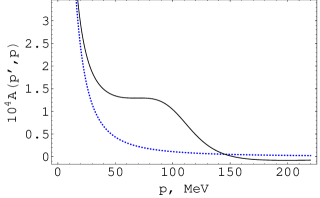
Figure 1: The real part of the half off-shell $T$-matrix as a function of the on-shell momenta $p$. The curves represent the real part of the amplitude $A(p^{\prime},p)=-\langle{\bf p}^{\prime}|T(E_{p}+i0)|{\bf p}\rangle$ ($|{\bf p}^{\prime}|=10$ $MeV$) obtained by solving the LS equation with the potential (66) at LO (dotted line) and NLO (solid line). The exponential regulator was employed with $\Lambda=150{\text{MeV}}$.

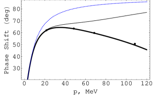
Figure 2: The ${}^{1}S_{0}$ phase shift of $NN$ scattering. Solid dots represent the experimental data Nijmegen . The dotted, solid and heavy solid curves represent the results obtained by using Eq. (V) with the LEC’s $c_{2}=8\cdot 10^{-5}\text{MeV}^{-2}$, ${\cal J}_{2}=-0.616$ and $c_{4}=-2\cdot 10^{-9}{\text{M}eV}^{-4},\quad{\cal J}_{4}=-8\cdot 10^{-5}{\text{M}eV}^{-2}$ at LO, NLO and NNLO, respectively.

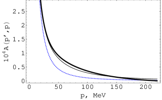
Figure 3: The real part of the half off-shell $T$-matrix as a function of the on-shell momenta $p$. The dotted, solid and heavy solid curves represent the solutions of the GDE for LEC’s $c_{2}=8\cdot 10^{-5}\text{MeV}^{-2}$, ${\cal J}_{2}=-0.616$ and $c_{4}=-2\cdot 10^{-9}{\text{M}eV}^{-4},\quad{\cal J}_{4}=-8\cdot 10^{-5}{\text{M}eV}^{-2}$ at LO, NLO and NNLO, respectively.

$V=\sum\limits_{\mu=0}^{\infty}V_{\mu}$ with $V_{\mu}$ being contact potentials breaks down at the scale $\Lambda\sim 1/\sqrt{ar_{0}}$ since at this scale $V_{0}\simeq V_{2}$. This result is very discouraging from the EFT point of view: The amplitudes should be expanded in powers of $(Q/\Lambda)^{\nu}$ where $\Lambda$ is a mass scale typical of the particles not included explicitly in the theory. In the low energy EFT, with the pion integrated out, one would expect $\Lambda\sim m_{\pi}$. The scale $\Lambda\sim 1/\sqrt{ar_{0}}$ at which the effective expansion of the $2N$ potential breaks down can hardly be called a typical QCD scale. For this reason in Ref. Kaplan it was proposed to expand not the potential but the Feynman amplitudes. This expansion was shown to converge up to the scale $\Lambda\sim m_{\pi}$. However, in this way one can calculate only the scattering amplitudes not the off-shell $T$-matrix. The advantage of the way of the expansion of the effective theory based on the formalism of the GQD is that it allows one to calculate not only the scattering amplitudes but also the off-shell $2N$ $T$-matrix, and its EFT expansion converges up to the expected scale set by the pion mass. But for this we must not restrict ourselves to the solution sets associated with potential model when the parameters $c_{2}$ and ${\cal J}_{2}$ are constrained not only by Eq. (72) but also by Eq. (69). Indeed, in general these LEC’s determining the solution set $\Omega_{2}$ must satisfy only Eq. (72). This means that fitting to the scattering data does not allow one to obtain these constants. However, it is natural to expect that the off-shell $T$-matrix must approach order by order to the true one with the same accuracy as the on-shell matrix elements that determine the phase shift. This puts some additional constraint on the values of the constants. Let us investigate the problem of the convergence of the effective expansion up to NNLO. At this order the $2N$ $T$-matrix is given by Eq. (52). For simplicity we will restrict ourselves to the case when the function $\Phi_{0}({\bf p}_{2},{\bf p}_{1})$ in Eq. (IV) is equal to zero, and the expression for the NNLO $2N$ $T$-matrix in the ${}^{1}S_{0}$ channel takes the form

$$\langle{\bf p_{2}}|T^{(4)}(z)|{\bf p_{1}}\rangle=\frac{(1+c_{2}^{*}p_{2}^{2}+c_{4}^{*}p_{2}^{4})(1+c_{2}p_{1}^{2}+c_{4}p_{1}^{4})}{C_{0}^{-1}-\frac{m}{4\pi}\sqrt{-zm}\Big{(}1+2\textsf{Re}c_{2}zm+\Big{[}|c_{2}|^{2}+2\textsf{Re}c_{4}\Big{]}(zm)^{2}\Big{)}+{\cal J}_{2}zm+{\cal J}_{4}(zm)^{2}}$$

$$\times\left(1+O\{Q^{5}/\Lambda^{5}\}\right),\quad|{\bf p}_{1}|<\Lambda,\quad|{\bf p}_{2}|<\Lambda.$$ (73)

This is a good approximation to the $2N$$T$-matrix because it has a pole near $E=0$ in the ${}^{1}S_{0}$ channel. The results of our calculations have shown that an acceptable convergence of the effective expansion is achieved in the case when the parameter $c_{2}$ is positive. For example, as we see from Figs. 3 and 4, convergence up to the expected scale takes place for the following set of the LEC’s: $C_{0}=-0.0016\text{MeV}^{-2}$ (fixed at LO); $c_{2}=8\cdot 10^{-5}\text{MeV}^{-2}$ and ${\cal J}_{2}=-0.616$ (fixed at NLO); $c_{4}=-2\cdot 10^{-9}{\text{M}eV}^{-4}$ and ${\cal J}_{4}=-8\cdot 10^{-5}{\text{M}eV}^{-2}$ (fixed at NNLO). Note that in this case we deal with the set of the solutions of the GDE that cannot be associated with any potential. This is because the condition (70) that can be satisfied in the case of the solutions obtained starting from the LS equation with the singular potential (65) allows only negative $c_{2}$. In fact, taking into account that in the ${}^{1}S_{0}$ channel $\frac{1}{2}ar_{0}=-(\frac{1}{35\text{MeV}})^{2}$, while $c_{2}$ is of order $\frac{1}{\Lambda^{2}}\sim(\frac{1}{m_{\pi}})^{2}$, from Eq. (71) we conclude that ${\cal J}_{2}$ is close to $-\frac{1}{2}ar_{0}C_{0}^{-1}$, and hence is negative. From Eqs. (67) and (70) than it follows that the constant must be negative.

For momentum $p\sim m_{\pi}$ explicit pion fields must be included in the theory. In this case in analyzing the time ordered diagrams for $2N$ $T$-matrix one has to take into account that the contributions from the ”$2N$ irreducible” diagrams manifest themselves not only as contact interactions but also as pion-exchange ones. In this context the $2N$ $T$-matrix obtained in the previous section should be considered as a contribution from the processes in which only contact interactions come into play. According to the Weinberg proposal this contribution should be obtained by iterating the corresponding contact potential in the LS equation. On the other hand, the solutions of the LS equation have the following asymptotic behavior

$$\langle{\bf p}_{2}|T(z)|{\bf p}_{1}\rangle\mathop{\to}\limits_{|z|\to\infty}\langle{\bf p}_{2}|V|{\bf p}_{1}\rangle,$$

which means that in the limit of high energies the $T$-matrix gets the dominant contribution from the potential. In our case, when this $T$-matrix describes the sum of contributions from the all relevant contact diagrams in ChPT and the potential is its ”$2N$ irreducible” part, the above should mean that this part gives the main contribution in the limit of high energies. However, this is not the case because all Feynman diagrams with $C_{0}$’s at each vertex give a contribution of the same order. In the chiral potential approach this problem is solved by putting in $ad$ $hoc$ short-ranged form factors in front of the contact interactions. As we have demonstrated, in the ${}^{1}S_{0}$ channel at NLO after renormalization of the solution of the LS equation with potentials regularized in this way we arrive at the expression (III) we have obtained, by using the GDE and the momentum dependence of the above sum of the contact diagrams that is given by Eq. (III) without extracting any potential. It can also be shown that renormalization of the solution of the LS equation with the NNLO contact potential gives rise to the expression (IV). However, as we have seen, there are solutions of the GDE consistent with symmetries of QCD that cannot be obtained by starting from the LS equation with regularized contact potentials. This is not surprising for the following reasons.

As is well known, the short-distance physics in ChPT is not the full short-distance physics of QCD. At distance scales $\sim 1/\Lambda_{\chi}$ mechanisms not encoded in ChPT will come into play, and will regulate the behavior of the nuclear forces at short distances. On the other hand, in quantum field theory, if we spread interaction in space, we spread it in time as well. Thus the processes that in describing low energy nucleon dynamics should be used as a short-range part of the $NN$ interaction are nonlocal in time. In the ordinary quantum mechanics nonlocality in time of an interaction, when it is used as a ”fundamental” interaction generating the dynamics of a system creates the conceptual problems with causality and unitarity. This is because the Shrödinger equation is local in time, and the interaction Hamiltonian describes an instantaneous interaction. As we have seen, the formalism of the GQD provides the extension of the quantum dynamics needed for solving this problem, and the GDE allows one to describe the evolution of a system with a nonlocal-in-time interaction. It is remarkable that such a nonlocalization can take place if and only if the UV behavior of the matrix elements of the evolution operator is ”bad”.

As we have shown, the requirement that the $2N$ $T$-matrix satisfies the GDE and has momentum behavior shown in Eq. (III) allows one to construct it order by order in the effective expansion. Note that at any order $\langle{\bf p}_{2}|T^{(2{\cal N})}(z)|{\bf p}_{1}\rangle$ constructed in this way satisfies the GDE and hence is unitary. The corresponding interaction operator describes the effective interaction that is spread not only in space but also in time. This manifests itself in the momentum and energy dependence of $\langle{\bf p}_{2}|B^{(2{\cal N})}_{eff}(z)|{\bf p}_{1}\rangle$. The regularization of the contact potentials spreads the interaction described by this potential only in space. Iterating this potential in the LS equation spreads the interaction also in time. So in the energy region relevant for describing low energy nucleon dynamics the effective interaction reproduced by the regularized potential is nonlocal in time. However, since this potential gives the main part of the contribution to the $T$-matrix only in the region much above the scale $\Lambda_{\chi}$ where the nonrelativistic two-nucleon LS equation is physically meaningless, in this case the solution of the LS equation is only of formal importance. To clarify this point note that the LS equation is equivalent to the Schrödinger equation that implies the existence of the infinitesimal generator of the group of the evolution operator $V(t)$. However, for the operator $(V(t,0)-1)/t$ to approach to the limiting one sufficiently close, one has to cross the region of times much below the time scale $1/\Lambda_{\chi}$. For such times, as it follows from Eqs. (13) and (14), the dominant contribution comes from the operators $T(z)$ corresponding to $z$ much above the scale $\Lambda_{\chi}$. This means that the dynamics is not governed by the Schrödinger equation formulated in the terms of low energy degrees of freedom. The above might be considered as an evidence of inconsistency of the cutoff approach, but the formalism of GQD provides a new reason to use the LS equation with a regularized potential:The solution of the LS equation with any regularized potential satisfies the condition (55), and hence the solution for $z\in{\cal D}$ can be used as the effective interaction operator in the GDE. In this case the existence of the infinitesimal generator of the group of the evolution operators is not required. However, as we have seen, not all the solutions of the GDE relevant for the problem can be obtained in the above way. In other words there are the interaction operators satisfying the condition (55) that cannot be represented as a formal solution of the LS equation with any regularized potential. The above means that it is possible that not all the effects of short-distance physics of QCD can be incorporated in the effective theory of nuclear forces in the standard way where the short-range part of the $NN$ interaction is described by the regularized contact potentials. This motivates a modification of the chiral potential model that could incorporate the description of the short-range interaction based on the use of the GDE.

In the theory with pions the interaction operator should contain terms describing both the short-range and long-range parts of the $NN$ interaction. In Ref. FizB it has been shown that at leading order in the ${}^{1}S_{0}$ channel the $NN$ interaction operator that is determined by the behavior of the $2N$ $T$-matrix in the energy region ${\cal D}$ where the dominant contributions to the $2N$ $T$-matrix come from the ”$2N$ irreducible” diagrams of ChPT is of the form

$$\langle{\bf p}_{2}|B^{(0)}(z)|{\bf p}_{1}\rangle=\langle{\bf p}_{2}|B^{(0)}_{sh}(z)|{\bf p}_{1}\rangle+\langle{\bf p}_{2}|V^{(0)}_{\pi}|{\bf p}_{1}\rangle,$$ (74)

where the potential $V^{(0)}_{\pi}$ is given by Eq. (V), i.e., is just the LO component of the long-range part of the chiral potentials, and $B^{(0)}_{sh}(z)$ describes the short-range component of the $NN$ interaction at LO and is given by Eq. (30). In the present paper we cannot discuss the theory with pions in detail. However, the arguments presented in Ref. FizB lead us to the conclusion that at any order the $2N$ interaction operator can be represented as a sum of the nonlocal-in-time short-range component being the sum of the relevant contact diagrams and instantaneous part that is the sum of the irreducible pion-exchange diagrams

$$\langle{\bf p}_{2}|B(z)|{\bf p}_{1}\rangle = \langle{\bf p}_{2}|B_{sh}(z)|{\bf p}_{1}\rangle+\langle{\bf p}_{2}|V_{\pi}|{\bf p}_{1}\rangle,$$ (75)

where the long-range component $\langle{\bf p}_{2}|V_{\pi}|{\bf p}_{1}\rangle$ may be describe by that of the chiral potential at the corresponding order. The solution of Eq. (8) with this interaction operator is not more complicated than the solution of the LS equation with an ordinary potential. In fact, the solution of Eq. (8) with the boundary condition (9) where $B(z)$ is given by Eq. (75) can be represented in the form

$$T(z)=T_{sh}(z) + \Big{(}1+T_{sh}(z)G_{0}(z)\Big{)}\tilde{T}_{\pi}(z)$$ (76)

$$\times \Big{(}1+G_{0}(z)T_{sh}(z)\Big{)},$$

where $T_{sh}(z)$ is the $T$-matrix describing the dynamics by $B_{sh}(z)$ alone, i.e., is the solution of equation

$$\frac{dT_{sh}(z)}{dz}=-\int\frac{d^{3}k}{(2\pi)^{3}}\frac{T_{sh}(z)|{\bf k}\rangle\langle{\bf k}|T_{sh}(z)}{(z-E_{k}+i0)^{2}},$$ (77)

with the boundary condition $T_{sh}(z)\mathop{\to}\limits_{|z|\mathop{\to}\infty}B_{sh}(z)$, and $\tilde{T}_{\pi}(z)$ satisfies the equation

$$\tilde{T}_{\pi}(z)=V_{\pi}+V_{\pi}G_{sh}(z)\tilde{T}_{\pi}(z),$$

$$G_{sh}(z)=G_{0}(z)+G_{0}(z)T_{sh}(z)G_{0}(z).$$ (78)

Note that, by using the ”two-potential trick” Newton , the solution of the LS equation with the potential $V=V_{sh}+V_{\pi}$ can be written just in the same form. The only difference is that in the latter case $T_{sh}(z)$ is the solution of the LS equation with the potential $V_{sh}(z)$, while in the general case where Eq. (V) is derived from the GDE with the interaction operator (75), $T_{sh}(z)$ is the solution of Eq. (V) with the interaction operator $B_{sh}(z)$.

At $NNLO$ the $NN$ interaction in the ${}^{1}S_{0}$ channel can be parametrized by the operator

$$\langle{\bf p}_{2}|B(z)|{\bf p}_{1}\rangle = \langle{\bf p}_{2}|B^{(2)}_{eff}(z)|{\bf p}_{1}\rangle+\langle{\bf p}_{2}|V_{\pi}|{\bf p}_{1}\rangle,$$ (79)

$$\langle{\bf p}_{2}|V_{\pi}|{\bf p}_{1}\rangle = \langle{\bf p}_{2}|V^{(0)}_{\pi}|{\bf p}_{1}\rangle$$ (80)

$$+ \langle{\bf p}_{2}|V^{(2)}_{\pi}|{\bf p}_{1}\rangle+\langle{\bf p}_{2}|V^{(3)}_{\pi}|{\bf p}_{1}\rangle,$$

where the operator $B_{eff}^{(2)}(z)$ is given by Eq. (IV), and $\langle{\bf p}_{2}|V^{(\nu)}_{\pi}|{\bf p}_{1}\rangle$ are the pion-exchange components of the chiral potential (61) projected to the ${}^{1}S_{0}$ state. Thus for the $NNLO$ $2N$ $T$-matrix in the ${}^{1}S_{0}$ channel we have

$$\langle{\bf p}_{2}|T(z)|{\bf p}_{1}\rangle=\langle{\bf p}_{2}|\left(T_{sh}^{(2)}(z)+T_{sh}^{(2)}(z)G_{0}(z)\right)\tilde{T}_{\pi}(z)$$ (81)

$$\times \left(1+G_{0}(z)T_{sh}^{(2)}(z)\right)|{\bf p}_{1}\rangle\left(1+O\left(\left\{Q/\Lambda\right)^{3}\right\}\right),$$

where $T_{sh}^{(2)}(z)$ is given by Eq. (III). At the same time, as we have shown, the result of resuming the contact potential (65) to all orders can be represented in the form (46) with the LEC’s given by Eqs. (69) and (70). In other words, there are the solution sets at which one can arrive starting from the $LS$ equation with the contact potential (65), and in the case when $T_{sh}^{(2)}(z)$ in Eq. (81) belongs to such sets this equation represents the $T$-matrix (more precisely a set of the $T$-matrices) that coincide with the $2N$ $T$-matrix obtained by solving the $LS$ equation with the $NNLO$ chiral potential.

Thus in the particular case the GDE with the interaction operator (79) can reproduce the same results as the LS equation with the $NNLO$ chiral potential. However, Eq. (81) that represents the solutions of the GDE with the interaction operator (79) allows a much wider class of the solutions, and only experiment can discriminate between them. As we show in the next section, the above freedom in choosing values of the LEC’s characterizing the short-range part of the $NN$ interaction allows one to significantly change the off-shell predictions of the model and at the same time to keep the $NN$ phase shifts unchanged. This gives us the hope that the above modification of the chiral potential model could increase their predictive power in describing few-body and microscopic nuclear structure problems where the off-shell properties of the $NN$ interaction play an important role.

VI Effects of the short-range forces on the off-shell 2N T-matrix and the pp bremsstrahlung

One of the simplest processes involving the half off-shell $NN$ interaction is proton-proton bremsstrahlung. Many years ago, it was suggested to use the bremsstrahlung process as a tool to discriminate between the various existing $2N$ potential models Ashkin . However, it has been shown that once all ingredients which are necessary for the calculation of the bremsstrahlung process are introduced, the predictions of various modern potential models do not differ significantly, independent of whether they are finite range or energy dependent Herrmann . The problem is that there is a significant discrepancy between these predictions and experimental data of KVI M-S for asymptotic proton angles: As was shown in Ref.M-S , the microscopic calculations reproduce the $pp\gamma$ cross sections reasonable well, however, for certain kinematics for which the final $pp$ system has a low kinetic energy, there is a significant over predictions of the data by about $20\%-30\%$. Since the discrepancy between the results of the microscopic calculations and the experimental results increases as the kinetic energy of outgoing protons decreases, one would speculate that including the Coulomb force might resolve the problem. However, it has been shown by Cozma et al. C-T that this is not the case. An important part of this discrepancy between theory and experiment originates in a poor description of the $NN$ interaction in the ${}^{1}S_{0}$ channel at low energies C-T . However, the above refers only to potentials model, while, as we have seen, there are such short-distance effects that can be represented by the GDE but not by any potential model. This leads us to the conclusion that the possible source of the discrepancy between the data and the microscopic calculations is the inability of the potential approach to incorporate such effects. Let us now examine this possibility in the same way that was used by Cozma et all C-T for investigating the effect of including the Coulomb interaction. In Ref. C-T this effect was studied by using the separable approximation to the $NN$ interaction. The form factor $g({\bf p})$ in the separable potential

$$V({\bf p}_{2},{\bf p}_{1})=\lambda g^{*}({\bf p}_{2})g({\bf p}_{1})$$ (82)

was chosen in the form

$$g({\bf p})=\frac{\beta^{2}}{p^{2}+\beta^{2}},$$

and the parameters $\lambda$ and $\beta$ were fixed by the scattering length $a$ and the effective range $r_{0}$. The Coulomb effect was investigated by adding the Coulomb potential to the separable potential, and these corrections was shown to be minor in the region needed for the KVI bremsstrahlung experiment.

Let us now, instead of the Coulomb effect, investigate the effects of the including the short-range NLO interaction operator $B^{(2)}_{sh}(z)$ given by Eq. (IV) in combination with the potential (82). In this case the interaction operator of our problem is of the form

$$\langle{\bf p}_{2}|B_{eff}(z)|{\bf p}_{1}\rangle=\langle{\bf p}_{2}|B_{sh}^{(2)}(z)|{\bf p}_{1}\rangle$$

$$+\lambda g^{*}({\bf p}_{2})g({\bf p}_{1}).$$ (83)

For such a choice of the interaction operator, Eq. (V) leads to the following $T$-matrix:

$$\langle{\bf p}_{2}|T(z)|{\bf p}_{1}\rangle=\frac{\psi_{0}^{*}({\bf p}_{2})\psi_{0}({\bf p}_{1})t_{sh}(z)+g^{*}({\bf p}_{2})g({\bf p}_{1})t_{\pi}(z)+\Big{(}\psi_{0}^{*}({\bf p}_{2})g({\bf p}_{1})I^{*}_{\pi sh}(z^{*})+g^{*}({\bf p}_{2})\psi_{0}({\bf p}_{1})I_{\pi sh}(z)\Big{)}t_{sh}(z)t_{\pi}(z)}{1-t_{sh}(z)t_{\pi}(z)I_{\pi sh}(z)I^{*}_{\pi sh}(z^{*})}$$ (84)

with

$$t_{sh}(z) = \frac{1}{C_{0}^{-1}-\frac{m}{4\pi}\sqrt{-zm}\Big{(}1+2\textsf{Re}c_{2}zm\Big{)}+{\cal J}_{2}zm}\left(1+O\{Q^{3}/\Lambda^{3}\}\right),$$

$$t_{\pi}(z) = \frac{1}{\lambda^{-1}-\int\frac{d^{3}k}{(2\pi)^{3}}\frac{|g({\bf k})|^{2}}{z-E_{k}}},$$

$$I_{\pi sh}(z) = \int\frac{d^{3}k}{(2\pi)^{3}}\frac{g({\bf k})\psi^{*}_{0}({\bf k})}{z-E_{k}}=\Big{[}\frac{m}{4\pi}\frac{\sqrt{-zm}-\beta}{1+zm/\beta^{2}}\Big{(}1+c^{*}_{2}zm\Big{)}-{\cal J}_{\pi sh}\Big{]}\Big{(}1+O\{Q^{3}/\Lambda^{3}\}\Big{)},$$ (85)

where

$${\cal J}_{\pi sh}=\frac{m}{2\pi^{2}}\int g({\bf k})\Big{(}\psi^{*}_{0}({\bf k})-1\Big{)}dk.$$ (86)

Here we restrict ourselves to the case where the function $\psi_{0}({\bf p})$ that occur in Eq. (III) is real. Equation (84) represents a set of the solutions of the GDE that coincide with the true $2N$ $T$-matrix with an accuracy of order $O\{Q^{3}/\Lambda^{3}\}$, because, as we noted, the effective operator $B^{(2)}_{sh}(z)$ represents a set of the operators describing the short-range part of the $NN$ interaction. Note that this solution set is determined not only by the LEC’s $C_{0}$, $c_{2}$, ${\cal J}_{2}$, $\beta$, and $\lambda$ that occur in the interaction operator (VI) but also by an additional constant ${\cal J}_{\pi sh}$. This means that really the operator (VI) being the sum of the short-range interaction operator and the potential $V_{\pi}$ is not so close to the true solution in the domain ${\cal D}$ to uniquely determine the set of the solutions of the GDE that coincides with an accuracy of order $O\{Q^{3}/\Lambda^{3}\}$. In Ref. FizB this situation was explained by using the example of the interaction operator (74) generating low energy nucleon dynamics at leading order. As it has been shown in Ref. FizB , at high $z$ this interaction operator is not so close to the true $2N$ $T$-matrix to uniquely determine the relevant solution. This means that the operator (74) does not satisfy the condition (55). By substituting the operator (74) into Eq. (55), one can obtain terms that should be added to the short-range part of the interaction operator FizB . In principle the interaction operator (VI) should be corrected in the same way. However, one may treat the interaction operator of the form (VI) keeping in mind that this operator does not determine a unique solution of the GDE (more precisely a unique solution set). Indeed, Eq. (84) represents a family of the solution sets: In general the solutions belonging to the sets with different values of the parameter ${\cal J}_{\pi sh}$ given by Eq. (86) do not coincide with each other with an accuracy of order $O\{Q^{3}/\Lambda^{3}\}$. So to select one of these sets we should chose the parameter ${\cal J}_{\pi sh}$. In general this parameter should appear in the above hidden additional terms, and the corrected interaction operator should determine a unique solution (solution set) of the GDE. Thus the set $\Omega_{2}$ of the solutions of the GDE that coincide with the true $2N$ $T$-matrix with an accuracy of order $O\{Q^{3}/\Lambda^{3}\}$ is determined by the LEC’s $C_{0}$, $c_{2}$, ${\cal J}_{2}$, ${\cal J}_{\pi sh}$ characterizing the short-range part of the $NN$ interaction and the constant $\beta$, and $\lambda$ parametrizing its long-range component. Each of the solutions belonging to this set corresponds to some definite function $\psi_{0}({\bf p})$ satisfying the conditions (24), (III) and (86) with given LEC’s $c_{2}$, ${\cal J}_{2}$ and ${\cal J}_{\pi sh}$, and for momenta below $\Lambda$ can be represented as

$$\langle{\bf p}_{2}|T(z)|{\bf p}_{1}\rangle = \Big{[}\frac{(1+c^{*}_{2}p_{2}^{2})(1+c_{2}p_{1}^{2})t_{sh}(z)+g^{*}({\bf p}_{2})g({\bf p}_{1})t_{\pi}(z)}{1-t_{sh}(z)t_{\pi}(z)I^{*}_{\pi sh}(z^{*})I_{\pi sh}(z))}$$ (87)

$$+ \frac{\Big{(}(1+c^{*}_{2}p_{2}^{2})g({\bf p}_{1})I^{*}_{\pi sh}(z^{*})+g^{*}({\bf p}_{2})(1+c_{2}p_{1}^{2})I_{\pi sh}(z)\Big{)}t_{sh}(z)t_{\pi}(z)}{1-t_{sh}(z)t_{\pi}(z)I^{*}_{\pi sh}(z^{*})I_{\pi sh}(z)}\Big{]}\Big{(}1+O\{Q^{3}/\Lambda^{3}\}\Big{)}.$$

The constants of the model can be obtained from the requirement that Eq. (87) reproduces observables with an accuracy of order $O\{Q^{3}/\Lambda^{3}\}$. Obviously the fitting to the $pp$ scattering data is not sufficient for this, because these constants determine not only the on-shell but also the off-shell properties of the $2N$ $T$-matrix. For their determination the comparison with experimental data such as the bremsstrahlung data in which the off-shell properties of the $NN$ interaction manifest themselves is needed. For example, one can use the $T$-matrix (87) for describing the elastic $2N$ $T$-matrix in the $pp\gamma$ model of Martinus et al. Martinus1 ; Martinus2 , and try to fit the constants to reproduce the experimental cross sections. However, in this paper we restrict ourselves to the investigation of the effects of the short-range interaction on the off-shell $2N$ $T$-matrix in the region needed for KVI bremsstrahlung experiment.

In Figs. 4,5,6, and 7 the results of the calculations of the $T$-matrix given by Eq. (87). The parameters $\lambda$ and $\beta$ characterizing the long range component of the interaction operator (VI) were determined by fitting the scattering amplitude reproduced by the pure potential model to the scattering length $a=-18.1{\text{fm}}$ and the effective range $r_{0}=2.60\text{fm}$. These values of $a$ and $r_{0}$ correspond to the case when the Coulomb interaction is switched off C-T . The results of our calculations plotted in Figs. 4 and 5 show that for some values of the LEC’s $c_{2}$, ${\cal J}_{2}$, and ${\cal J}_{\pi sh}$ the difference between the half off-shell amplitudes $\langle{\bf p}_{1}|T(E_{p}+i0)|{\bf p}\rangle$ with and without the short range corrections becomes larger as the momentum going from the on-shell point, while, as we see from Fig. 4, including the contact term keeps the phase shift unchanged. In contrast, as has been shown in Ref. C-T , the Coulomb corrections become minor for high off-shell momenta, and hence cannot remove the discrepancy between theory and experiment in describing the $pp\gamma$ process. Our results show that with an appropriate choice of the constants the short range part of the $NN$ interaction gives a significant contribution to the $2N$ $T$-matrix in the case when the laboratory kinetic energy $E_{\text{lab}}$ of the outgoing protons is below $15$ $MeV$ and the off-shell momentum is sufficiently high. This is just the region needed for the KVI bremsstrahlung experiment.

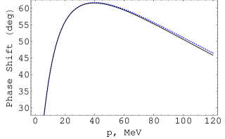
Figure 4: A comparison between the $pp$ phase shifts (${}^{1}S_{0}$ channel) for the potential (82) fitted to $a=-18.1$ fm and $r_{e}=2.60$ fm (dotted line) and the predictions of the model corrected by including the short effects (solid line).

Figure 5: The $T$-matrix as a function of the off-shell momentum $p$ at a laboratory energy of $10$ MeV. The solid and dashed curves represent, respectively, the real and imaginary parts of the normalized $T$-matrix $\langle p|T_{\pi}(E_{k}+i0)|k\rangle/|\langle 0|T_{\pi}(E_{k}+i0)|k\rangle|$, where $T_{\pi}(z)$ is the solution of the LS equation with the potential (82). The heavy solid and bold type dashed curves represent, respectively, the real and imaginary part of $\langle p|T(E_{k}+i0)|k\rangle/|\langle 0|T_{\pi}(E_{k}+i0)|k\rangle|$, where $T(z)$ is given by Eq. (84). The parameters are following $\beta=241.468\text{MeV}$, $\lambda=-1.0269\cdot 10^{-4}\text{MeV}^{-2}$, $C_{0}=1.29\cdot 10^{-4}\text{MeV}^{-2}$, ${\cal J}_{\pi sh}=-17942{\text{MeV}}^{2}$, $c_{2}=2.3\cdot 10^{-7}\text{MeV}^{-2}$, ${\cal J}_{2}=2.75$.

Figure 6: The difference $\Delta(E_{\text{lab}},p)$ between the predictions of the model with and without the short-range corrections for the T-matrix in the region needed for the KVI experiment ($p=300$ MeV).

Figure 7: Same as Fig. 6 but for $p=500$ MeV.

A large discrepancy between experiment and the predictions of the potential models appears in the kinematical regions where the cross section has peaks. The presence of these peaks is the result of strong final-state interaction at small values of the kinetic energy of outgoing protons ($E_{\text{lab}}<15\text{MeV}$). This means that the over prediction of the potential models in describing the $pp\gamma$ cross sections may be a reflection of the fact that really the $NN$ interaction at low energies is not so strong as it is predicted by the potential models. In Figs. 6 and 7 we plot the relative difference

$$\Delta(E_{\text{lab}},p^{\prime})=\frac{|\langle{\bf p}^{\prime}|T_{\pi}(E_{p}+i0)|{\bf p}\rangle|-|\langle{\bf p}^{\prime}|T(E_{p}+i0)|{\bf p}\rangle|}{|\langle{\bf p}^{\prime}|T(E_{p}+i0)|{\bf p}\rangle|},$$

$E_{\text{lab}}=2p^{2}/m$, between predictions of the model with and without the short-range component for the half off-shell $T$-matrix where $T_{\pi}(z)$ is the solution of the $LS$ equation with the potential (82). As we see, for high off-shell momenta, the magnitude of $\Delta(E_{\text{lab}},p)$ characterizing the effect of the short-range forces on the $2N$ $T$-matrix grows rapidly as the energy $E_{\text{lab}}$ going to zero in the region $E_{\text{lab}}<15$ MeV. Note that in this kinematic region the difference between the predictions of the microscopic models for bremsstrahlung and the KVI experimental data has just the same energy dependence M-S . This leads us to the conclusion that the improvement of the low-energy part of the strong interaction that can be achieved by correcting its short-range component may remove the discrepancy between theory and experiment. However, for including the short-range component to give rise to the above effect, the constants $c_{2}$ and ${\cal J}_{2}$ should have such values that are inconsistent with any potential model. In fact, if the LEC’s $c_{2}$ and ${\cal J}_{2}$ correspond to some contact potential then they must be related by Eq. (70). From this it follows that for $c_{2}=2.3\cdot 10^{-7}\text{MeV}^{-2}$ and ${\cal J}_{2}=2.75$ which lead to the results shown in Figs. (4-7) the integral $\int d\tilde{k}|f(\tilde{k})|^{2}$ should be of order $\sim\frac{{\cal J}_{2}\pi^{2}}{c_{2}m\Lambda_{\chi}}=1.26\cdot 10^{5}\Lambda_{\chi}^{-1}$, where the cutoff is set by the chiral symmetry breaking scale $\Lambda_{\chi}=1GeV$. However, such a size of this integral is inconsistent with the fact that the regulator function $f(k/\Lambda)$ must satisfy $f(0)=1$ and fall off rapidly for $k/\Lambda>1$. This means that the effective $2N$ $T$-matrix (87) corresponding to the above LEC’s cannot be associated with any potential.

The above model can be considered as a combination of the standard nuclear physics approach based on the use of the $NN$ potentials and the effective theory of nuclear forces. As we have seen, combining our approach to the description of the short-range part of the $NN$ interaction with the separable potential model yields very encouraging results in investigating possible origins of the discrepancy between the theoretical predictions for the $pp$ bremsstrahlung and experiment. In the same way one can construct a more realistic model by replacing the potential (82) in Eq. (VI) with one of the high precision phenomenological $NN$ potentials [25-30]. These potentials contain the terms describing the short-range part of the $NN$ interaction, and hence in this case the operator $B_{sh}(z)$ in Eq. (74) should be considered as a correction to the model dependent short-range components of the realistic potentials in which the ambiguous short-distance parametrization is used. It is important that such corrections may allows one not only to remove or minimize the model dependence but also improve the description of the off-shell properties of the $NN$ interaction that is needed for removing the discrepancy between the theory and the experiment in describing the $pp$ bremsstrahlung.

VII The off-shell behavior of the $2N$ $T$-matrix and the three-nucleon problem

As we have shown, our formulation of the effective theory of nuclear forces allows one to construct, as an inevitable consequence of the basic principles of quantum mechanics and symmetries of QCD, not only the $2N$ scattering amplitude (in this case we reproduce all results of the standard subtractive EFT approach), but also the off-shell $T$-matrix, and hence the evolution and Green operators. The advantage of this formulation over the tradition potential approach is that it allows one to take into account the constraints on the off-shell properties of the $NN$ interaction put by the symmetries of QCD. This is very important, because, as is well known, the off-shell behavior of the $2N$ $T$-matrix may play a crucial role in solving the many-nucleon problem and is an important factor in calculating in-medium observables Fuchs and in microscopic nuclear structure calculations. This results, for example, in the fact that the predictions by the Bonn potential for nuclear structure problems differ in a characteristic way from the ones obtained with local realistic potentials Machleidt . The off-shell ambiguities of realistic $NN$ potentials are argued to be one of the main causes of many problems in describing three-nucleon systems.

The modern potential models that describe $2N$ scattering data to high precision can not guarantee that a similar precision will be achieved in the description of larger nuclear systems. In fact, the simplest observable in the $3N$ system, the binding energy of the triton, is under predicted by the realistic $NN$ potentials which are so successful in describing the $2N$ observables. The energy deficit ranges from 0.5 to 0.9 MeV and depends on the off-shell and short-range parametrization of the $2N$ force Kievsky . In order to resolve this problem one has to take into account three-nucleon force (3NF) contributions to the $3N$ binding energy. The common way of solving the $3N$ bound state problem is to use in the Schrödinger equation phenomenological $NN$ potentials and then to introduce a 3NF to provide supplementary binding. However, from the point of view of the three-nucleon problem, it is not sufficient to generate a phenomenological $NN$ potential that perfectly reproduces the $2N$ scattering amplitudes. One must also generate a $NN$ potential by using theoretical insight as much as possible in order to constrain the off-shell properties of the $2N$ $T$-matrix. If this is not the case, a $NN$ potential which fits precisely the $2N$ phase shifts but produces the erroneous off-shell behavior of the $T$-matrix would not provide reliable results for the $3N$ system, nor can be used to test for the presence of $3N$ forces.

The models for the $3N$F that are usually used for solving the problem with the triton understanding are based on two-pion exchange with intermediate $\Delta$-isobar excitation. However, these $3N$F models cannot explain the $A_{y}$ puzzle which refers to the inability to explain the nucleon vector analyzing power $A_{y}$ in elastic nucleon-deuteron ($Nd$) scattering at low energy. As has been shown in Ref. Huber , it is not possible with reasonable changes in realistic $NN$ potentials to increase the $Nd$ $A_{y}$ and at the same time to keep the $2N$ observables unchanged. The same situation also takes place in the case of chiral potentials Entem . This means that the introduction of three-nucleon forces (3NF) is needed for resolving the problem. However, as it turned out, conventional $3N$F’s change the predictions for $Nd$ $A_{y}$ only slightly and do not improve them [36-38]. This motivated new types of $3N$F’s [39-41]. On the other hand, reliable $3N$ calculations and even testing for the presence of $3N$ forces require to constrain the off-shell properties of the $2N$. Moreover, these properties play a crucial role in a new $3N$F proposed by Canton and Schadow Canton . In Ref. Canton2 this $3N$F has been suggested as a possible candidate to explain the $A_{y}$ puzzle. The $3N$F contribution from this force is fixed by the $2N$ $T$-matrix describing the underlying 2N interaction while the pion is ”in flight”. The expression for this $3N$F derived in Ref. Canton contains the off-shell $2N$ $T$-matrix, more precisely its subtracted part

$$\tilde{t}_{12}({\bf p}_{2},{\bf p}_{1},z)=t_{12}({\bf p}_{2},{\bf p}_{1},z)-v_{12}({\bf p}_{2},{\bf p}_{1}),$$ (88)

where ${\bf p}_{1}$ and ${\bf p}_{2}$ are Jacobi momenta of nucleons 1 and 2, and the potential - like term $v_{12}({\bf p}_{2},{\bf p}_{1})$ contains only OPE/OBE - type diagrams. The subtraction in Eq. (88) is needed to take into account a cancellation effect which has been observed in Refs. Yang ; Yang2 . This cancellation involves meson retardation effects of the iterated Born term, and the irreducible diagrams generated by sub-summing all time ordering diagrams describing the combined exchange of two mesons amongst the three nucleons. In principle there are no free parameters to adjust, and the $3N$ force is completely determined by the $2N$ $T$-matrix. However, as has been shown in Ref. Canton2 , in order to explain the $A_{y}$ puzzle, instead of the subtracted $T$-matrix shown in Eq. (88), one has to use the amplitude defined according to the prescription

$$\tilde{t}_{12}({\bf p}_{2},{\bf p}_{1},z)=c(z)t_{12}({\bf p}_{2},{\bf p}_{1},z)-v_{12}({\bf p}_{2},{\bf p}_{1}),$$

with the effective parameter $c(z)$, which represents an overall correction factor for the far-off-shell $2N$ $T$-matrix. Ideally, this parameter should be one for the $2N$ potential to provide a reliable extrapolation of the $2N$ $T$-matrix down to $z\approx-160$ MeV. However, as has been shown in Ref. Canton2 , none of the existing $2N$ $T$-matrices can guarantee the off-shell behavior that is needed for the explanation of the $A_{y}$ puzzle with the parameter $c(z)$ set to one, since they are all constrained by such data the deuteron pole and the $2N$ phase shifts. For example, in order to reproduce the $nd$ experimental data with the Bonn B potential, the factor $c(z)$ must be set to $0.73$ for the energy $10$ $MeV$.

The above gives us the expect that the origin of discrepancy between the theory and experiment in describing $A_{y}$ is the same as in the case of the $pp$ bremsstrahlung: The potential models cannot reproduce the relevant off-shell behavior of the $2N$ $T$-matrix. This should mean that the answer lies beyond these models. The advantage of the formulation of the effective theory is that it allows one to constrain the possible $T$-matrix by the symmetries of QCD, but at the same time, permits the solutions that cannot be reproduced by any potential model. This opens new possibilities to resolve the $A_{y}$ puzzle. Note that the generalization of the above results to the $P$ waves needed for solving this problem is straightforward.

VIII Summary and Discussion

We have shown that from the Weinberg analysis of time-ordered diagrams for the $2N$ $T$-matrix in ChPT it follows that nucleon dynamics at low energies is governed by the GDE with a nonlocal-in-time interaction operator. A remarkable feature of the GDE which follows straightforwardly from the first principles of quantum mechanics is that it allows one to construct all physical amplitudes relevant for the theory under consideration by using the amplitudes describing processes in which the duration time of interaction is infinitesimal. It is natural to assume that the most of contribution to these amplitudes comes from the processes associated with a fundamental interaction in a quantum system. This point manifests itself in the boundary condition (3). If we do not consider a theory that is valid up to infinitely high energies (infinitesimal times), then the duration times of interaction much below the time scale of low energy physics but much above the scale of underlying high energy physics should be considered as ”infinitesimal”, and the operator describing the processes with such duration times of interaction can be used as an interaction operator. This in turn means that the amplitudes describing this ”fundamental” interaction in the low energy theory can be computed in terms of the underlying high energy physics.

The GDE can be represented in the form of the differential equation (8) for the operator $T(z)$. The boundary condition on this equation is shown in Eq. (9), where the operator $B(z)$ describes the fundamental interaction in this system. By definition, this operator must be so close to the true $T$-matrix in the limit $|z|\to\infty$ that the GDE with the boundary condition (9) have a unique solution. The above means that really this region of ”infinite” energies with which we have to deal is the domain ${\cal D}$ that lies much above the scale of the low energy dynamics but much below the scale of the underlying high energy physics. Correspondingly for describing the low energy dynamics we have to start with the boundary condition (54) that implies that the interaction operator $B(z)$ is so close to the relevant $T$-matrix inside the domain ${\cal D}$ that Eq. (8) with this initial condition has a unique solution. In the theory of nuclear forces this domain is a region of energies that are high enough for the most of contribution to the $2N$ $T$-matrix to come from processes that are described by the irreducible $2N$ diagrams for the $2N$ $T$-matrix (these processes are associated with a ”fundamental” interaction), but not so high for the heavy degrees of freedom manifest themselves explicitly. By using the analysis of the time-ordered diagrams for the $2N$ $T$-matrix in ChPT inside the domain ${\cal D}$ where the structure of the theory is much simpler than in the low energy region, we can obtain the $NN$ interaction operator which should be used in the boundary condition (54) on Eq. (8). We have shown that the dynamics which is generated by the interaction operator obtained in this way is non-Hamiltonian. This is because, for low energy nucleon dynamics to be Hamiltonian, the operator $T(z)$ must have a negligible dependence on $z$ inside the domain ${\cal D}$, while, as we have shown, this is not the case. In other words, in the nonrelativistic limit QCD leads through ChPT to low energy nucleon dynamics that is not governed by the Schrödinger equation. However, this does not mean that the low energy predictions of QCD are not consistent with quantum mechanics: Only the GDE must be satisfied in all the cases. We have shown that the requirement that the $2N$ $T$-matrix satisfies the GDE as a well defined equation free from UV divergences and has the structure consistent with the symmetries of QCD allows one to construct it order by order in the effective theory expansion without resorting to regularization and renormalization.

The above point is illustrated in detail by using the pionless theory of nuclear forces. For the ${}^{1}S_{0}$ channel $2N$ $T$-matrix that, as it follows from the Weinberg analysis, should be of the form (III), we have derived Eq. (III). This equation allows one to obtain the $2N$ $T$-matrix with an accuracy of order $O\{(Q/\Lambda)^{2{\cal N}+1}\}$ if it is known with an accuracy of order $O\{(Q/\Lambda)^{2{\cal N}-1}\}$. In this way at any order one can obtain the most general possible $2N$ $T$-matrix consistent with the symmetries of QCD. At NLO this $T$-matrix is given by Eq. (III). This equation represents the set $\Omega_{2}$ of the solutions of the GDE that coincide with the true $2N$ $T$-matrix with the accuracy up to order $O\{Q^{3}/\Lambda^{3}\}$. This solution set is generated by the effective interaction operator (IV). The fact that we have to deal with the set of the solutions means that at this order our knowledge about the details of the $NN$ interaction is not sufficient for discriminating between them. The set $\Omega_{2}$ is determined by the LEC’s $C_{0}$, $c_{2}$, and ${\cal J}_{2}$ that parametrize the effects of the high energy physics on low energy nucleon dynamics. It is shown that, the $2N$ $T$-matrix obtained in this way leads to the KSW expansion of the scattering amplitude Kaplan2 shown in Eq. (III). However, in contrast with the standard subtractive approach to the EFT of nuclear forces where this expansion is obtained by summing the bubble diagrams and performing regularization and renormalization, we reproduce the same results in a consistent way free from UV divergences. At NNLO the $2N$ $T$-matrix is given by Eq. (50). This equation represents the set $\Omega_{4}$ of the solutions of the GDE that coincide with the true $2N$ $T$-matrix with an accuracy of order $O\{Q^{5}/\Lambda^{5}\}$. In the same way one can obtain the solution set $\Omega_{2{\cal N}}$ that coincide with the true $2N$ $T$-matrix with the accuracy up to order $O\{(Q/\Lambda)^{2{\cal N}+1}\}$. As ${\cal N}$ increases the set $\Omega_{2{\cal N}}$ becomes smaller and smaller, i.e., one approaches to the true $2N$ $T$-matrix closer and closer.

The above strategy can be also used for constructing the $T$-matrix in the theory with pions. Another way of applying the results obtained in the paper is to use them in combination with the chiral potential approach. We have shown that at NNLO the $NN$ interaction in the ${}^{1}S_{0}$ channel can be parameterized by the operator (79). The solution of the GDE with this interaction operator is given by Eq. (81). In the particular case when the short-range part of the $2N$ $T$-matrix $T_{sh}^{(2)}(z)$ that enters in Eq. (81) can be associated with some potential model this equation leads to the same results as the chiral model with the NNLO potential. At the same time, as we have seen, there are such LEC’s characterizing the short-range part of the interaction operator (79) in the case of which $T_{sh}^{(2)}(z)$ cannot be associated with any potential model, and Eq. (81) gives rise to the $2N$ $T$-matrix that cannot be reproduced by the LS equation with the NNLO chiral potential. Thus, being equivalent to the chiral potential model in a particular case, above model allows one to go beyond the potential models, and such an extension of the standard chiral approach may be necessary to remove the discrepancy between the theory and experiment still existing in nuclear physics. This point has been illustrated by using the example of the model where the long-range part of the interaction is described by the potential (82). This is the model that in Ref. C-T was used for investigating the effects of including the Coulomb interaction on the $pp\gamma$ process where the Coulomb potential is replaced by the short-range interaction operator (VI). By using this model we have shown that, as we see from Figs. 6 and 7, there are such LEC’s for which the effect of the short-range interaction on the half off-shell $T$-matrix $\langle{\bf p}_{1}|T(E_{p}+i0)|{\bf p}\rangle$ grows rapidly as the kinetic energy of outgoing protons decreases in the region needed for KVI experiment. Note that just for such LEC’s the short-range interaction that is described by Eq. (III) cannot be associated with any potential. Such an effect of including the short-range interaction might seem very surprising, but the difference between the predictions of the potential models and experiment in this kinematic region grows in the same way. This lead us to the conclusion that the inability of the potential models to incorporate the short-distance effects which manifest themselves when we consider the problem from the point of view of the more general approach based on the use of the GDE, may be the source of the over prediction of the potential models in describing the $pp\gamma$ cross section. As we see from Figs. 4,5,6, and 7, these effects can improve the off-shell behavior of the $2N$ $T$-matrix and the same time keep the phase shift unchanged. This allow one to incorporate the above effects into the machinery based on the use of the high precision potentials keeping the phase shifts predicted by these potentials unchanged. As we noted, in this case the operator $B_{sh}(z)$ should describe corrections to these short-range components. One may hope that such an improvement of the description of the $NN$ interaction will make it possible to remove the discrepancy between theory and experiment in describing the $pp$ bremsstrahlung. Taking into account the above effects of the short-range interaction on the off-shell properties of the $2N$ $T$-matrix may also open new possibilities for explaining the $A_{y}$ puzzle.

References

- (1) S. Weinberg, Phys. Lett. B 251 288 (1990); Nucl. Phys. B 363, 3 (1991).
- (2) S.R. Beane, P.F. Bedaque, W.C. Haxton, D.R. Phillips and M.L. Savage, nucl-th/0008064.
- (3) S. Weinberg, hep-th/9702027.
- (4) R.Kh. Gainutdinov, J. Phys. A 32, 5657 (1999).
- (5) R.P. Feynman, Rev. Mod. Phys. 20, 367 (1948).
- (6) R.Kh. Gainutdinov and A.A. Mutygullina, Phys. Rev. C 66, 014006 (2002).
- (7) R.Kh. Gainutdinov, A.A. Mutygullina and W. Scheid, Phys. Lett. A 306, 1 (2002).
- (8) M.Mahjour-Shafiei et al., Phys. Rev. C 70, 024004 (2004).
- (9) M.D. Cozma, O. Scholten, R.G.E. Timmermans, and J.A. Tjon, Phys. Rev. C 68, 044003 (2003).
- (10) C. Ordòñez, L. Ray, and U. van Kolck, Phys. Rev. Lett. 72, 1982 (1994).
- (11) U. van Kolck, Prog. Part. Nucl. Phys. 43, 337 (1999).
- (12) D.R. Entem and R.Machleidt, Phys. Rev. C 68, 041001(R) (2003).
- (13) R.P. Feynman, The Theory of Fundamental Processes. W.A. Benjamin, INC, New York (1961).
- (14) D.B. Kaplan, M.J. Savage, and M.B. Wise, Phys. Lett. B 424, 390 (1998); Nucl. Phys. B 534, 329 (1998).
- (15) D.B. Kaplan, M.J. Savage and M.B. Wise, Nucl. Phys. B 478, 629 (1996).
- (16) U. van Kolck, Nucl. Phys. A 645, 273 (1999).
- (17) E. Epelbaum, W. Gl ckle, and U.-G. Meisner, Nucl. Phys. A 637, 107 (1998).
- (18) V.G.J. Stoks, R.A.M. Klomp, M.C.M. Rentmeester, and J.J. de Swart, Phys. Rev. C 48, 792 (1993).
- (19) R.Kh. Gainutdinov and A.A. Mutygullina, Fizika B 13, 373-382 (2004).
- (20) R.G. Newton, Scattering Theory of Waves and Particles, (Springer-Verlag, New york, 1982).
- (21) J. Ashkin and R. Marshak, Phys. Rev. 76, 58 (1949); M.I. Sobel and A.H. Cromer, ibid. 132, 2698 (1963); M.K. Lion and M.I. Sobel, Ann. Phys. (NY) 72, 323 (1972).
- (22) V. Herrmann and K. Nakayama, Phys. Rev. C 45, 1450 (1992).
- (23) G.H. Martinus, O. Scholten, and J.A. Tjon, Phys. Lett. B 402, 7 (1997); Few-Body Syst. 26, 197 (1999); G.H. Martinus, Ph.D. thesis, University of Groningen, 1988.
- (24) G.H. Martinus, O. Scholten, and J.A. Tjon, Phys. Rev. C 56, 2945 (1997).
- (25) M. Lacombe, B. Loiseau, J. M. Richard, R. Vinh Mau J. Côté, P. Pirès, and R. de Tourreil M. Lacombe et al., Phys. Rev. C 21, 861 (1980).
- (26) R. Machleidt, K. Holinde, and C. Elster, Phys. Rep. 149, 1 (1987).
- (27) R. Machleidt, F. Sammarruca, and Y. Song, Phys. Rev. C 53, 1483 (1996).
- (28) R. Machleidt, Phys. Rev. C 63,024001 (2001).
- (29) V.G.J. Stoks et al., Phys. Rev. C 49, 2950 (1994).
- (30) R.B. Wiringa, V.G.J. Stoks, and R. Schiavilla, Phys. Rev. C 51, 38 (1995).
- (31) C. Fuchs, A. Faessler, and M. El-Shabshiry, Phys. Rev. C 64, 024003 (2001)
- (32) R. Machleidt, Phys. Rev. C 63, 024001 (2001).
- (33) A. Kievsky, S. Rosati, W. Tornow, and M. Viviani, Nucl. Phys. A 607, 402 (1996).
- (34) D. Hüber and J. L. Friar, Phys. Rev. C 58, 674 (1998).
- (35) D.R. Entem, R.Machleidt, and H. Witala, Phys. Rev. C 65, 064005 (2002).
- (36) A. Kievsky, M. Viviani, and S. Rosati, Nucl. Phys. A 577, 511 (1994).
- (37) D. Hüber, H. Witala, and W. Glöckle, Few-Body Syst. 14, 171 (1993).
- (38) H. Witala, D. Hüber, and W. Glöckle, Phys. Rev. C 49, R14 (1994).
- (39) D. Hüber, J. L. Friar, A. Nogga, H. Witala, and U. van Kolck, Few-Body Syst. 26, 1 (1999).
- (40) J. L. Friar, Nucl. Phys. A 684, 200 (2001).
- (41) D. Hüber, J. L. Friar, A. Nogga, H. Witala, and U. van Kolck, Few-Body Syst. 30, 95 (2001).
- (42) L. Canton and W. Schadow, Phys. Rev. C 62, 044005 (2000).
- (43) L. Canton and W. Schadow, Phys. Rev. C 64, 031001 (2001).
- (44) S.N. Yang and W. Glöckle, Phys. Rev. C 33, 1774 (1986).
- (45) S.A. Coon and J. L. Friar, Phys. Rev. C 34, 1060 (1986).