Azimuthally Sensitive Femtoscopy and $v_{2}$

Abstract

I investigate the correlation between spatial and flow anisotropy in determining the elliptic flow and azimuthal dependence of the HBT correlation radii in non-central nuclear collisions. It is shown that the correlation radii are in most cases dominantly sensitive to the anisotropy in space. In case of $v_{2}$, the correlation depends strongly on particle species. A procedure for disentangling the spatial and the flow anisotropy is proposed.

1 Motivation

In non-central nuclear collisions at RHIC energies, the resulting fireball can exhibit anisotropy in both spatial shape and transverse expansion velocity profile. They both influence the measured “elliptic flow” coefficient $v_{2}$ vol . A question arises: how are they correlated in the determination of $v_{2}$, i.e., which combinations of spatial and flow anisotropy lead to the same elliptic flow?

On the other hand, dependence of HBT correlation radii on the azimuthal angle is also shaped by the two mentioned anisotropies. Therefore, the same question can be asked: how do the spatial anisotropy and transverse expansion flow anisotropy combine in the $\phi$-dependence of correlation radii?

An analogical situation appears in determining the slopes of single-particle $p_{T}$-spectra. It is well known that they are determined by temperature and transverse expansion velocity and that it is impossible to disentangle these two quantities from a single measured spectrum. There is, however, also the $M_{T}$-dependence of HBT radii in which the correlation of temperature and transverse flow is qualitatively different from that in the determination of spectra. Temperature and transverse flow velocity then can be unambiguously measured from analysing both spectra and HBT radii.

A similar solution shall be sought here: can we disentangle spatial and flow anisotropy in non-central collisions by analysing both $v_{2}$ and the azimuthally sensitive HBT radii?

Note that several statements have been made in literature which are related to this programme. In st130 the STAR collaboration concluded that it was impossible to determine spatial anisotropy just from the measurement of $v_{2}$ and a conjecture was made that HBT analysis would be able to gain such result. Two qualitatively different final states resulted from hydrodynamic simulations by Heinz and Kolb khplb and the authors demonstrated the possibility to distinguish these states by HBT interferometry. Here I report on a systematic study of the interplay between spatial and flow anisotropy in framework of generalisations of the blast-wave model.

2 An azimuthally anisotropic blast-wave model

Instead of fully describing the used model I will just focus on those features which are important for this work and refer the reader to literature for more detailed discussion retiere ; asym . Suffice it to say that the fireball is thermalised with a temperature $T$ and exhibits longitudinally boost-invariant expansion. Its transverse profile is ellipsoidal and the emission function is

$$S(x,p)\propto\Theta(1-\tilde{r})\,,\qquad\tilde{r}=\sqrt{\frac{x^{2}}{R_{x}^{2}}+\frac{y^{2}}{R_{y}^{2}}}\,,$$ (1)

where $R_{x}$ and $R_{y}$ are the two transverse radii, in and out-of-plane, respectively. They can be parametrised with the help of a spatial anisotropy parameter $a$

$$R_{x}=a\,R\,,\qquad R_{y}=\frac{R}{a}\,.$$ (2)

Thus an out-of-plane elongated source is characterised by $a<1$, whereas for an in-plane elongated source we have $a>1$.

The transverse expansion velocity also depends on the azimuthal angle. The velocity is given as

$$v_{\perp}=\tanh\rho(\tilde{r},\,\phi)\,.$$ (3)

We shall have a closer look at two models which differ in the azimuthal variation of the velocity. In Model 1 retiere the velocity is always perpendicular to a surface given by $\tilde{r}=\mbox{const}$. This direction together with the reaction plane defines the azimuthal angle $\phi_{b}$, as illustrated in Figure 1.

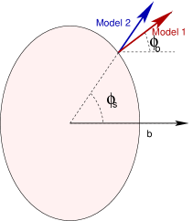
Figure 1: The two different models for transverse expansion velocity used here.

The transverse rapidity

$$\rho(\tilde{r},\phi)=\tilde{r}\,\rho_{0}\,(1+\rho_{2}\,\cos(2\phi_{b}))\,,$$ (4)

where the parameter $\rho_{0}$ measures the radial flow and $\rho_{2}$ is the flow anisotropy parameter. As the velocity is perpendicular to the surface of the fireball, this model resembles the expansion profile early in the fireball evolution: the direction of velocity coincides with acceleration which in turn is given by the pressure gradient.

In Model 2 the transverse expansion velocity is directed radially and varies with the usual azimuthal angle, which is denoted as $\phi_{s}$ here

$$\rho(\tilde{r},\phi)=\tilde{r}\,\rho_{0}\,(1+\rho_{2}\,\cos(2\phi_{s}))\,.$$ (5)

3 The elliptic flow

Recall that $v_{2}$ is defined as the second Fourier coefficient of the azimuthal dependence of spectrum

$$P_{1}(p_{T},\phi)=\left.\frac{d^{3}N}{p_{T}\,dp_{T}\,dy\,d\phi}\right|_{y=0}=\frac{1}{2\pi}\,\left.\frac{d^{2}N}{p_{T}\,dp_{T}\,dy}\right|_{y=0}\left(1+2v_{2}(p_{T})\cos(2\phi)+\dots\right)\,.$$ (6)

It can be calculated in the two used models and the result reads asym

$$v_{2}=\frac{\int_{0}^{1}d\tilde{r}\,\tilde{r}\int_{0}^{2\pi}d\phi\,\cos(2\phi)\,J(\phi)\,K_{1}(a)\,I_{2}(b)}{\int_{0}^{1}d\tilde{r}\,\tilde{r}\int_{0}^{2\pi}d\phi\,J(\phi)\,K_{1}(a)\,I_{0}(b)}\,,$$ (7)

where the arguments of the Bessel functions are $a=m_{T}\,\cosh\rho(\tilde{r},\phi)/T$ and $b=p_{T}\,\sinh\rho(\tilde{r},\phi)/T$. The only difference between the two models appears in the Jacobian $J(\phi)$

$$\mbox{Model 1:}\qquad J(\phi) = (a^{2}\cos^{2}\phi+a^{-2}\sin^{2}\phi)\,,$$ (8a)

$$\mbox{Model 2:}\qquad J(\phi) = (a^{-2}\cos^{2}\phi+a^{2}\sin^{2}\phi)\,.$$ (8b)

From these relations it is obvious that the two models lead to the same $v_{2}$ if they are related by transformation $a\to a^{-1}$. In other words, one in-plane and another out-of-plane source give the same $v_{2}$. This is an analytic illustration of the claim that it is impossible to determine even the qualitative type of spatial anisotropy just from measurement of $v_{2}$.

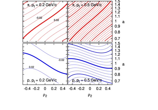
Figure 2: Elliptic flow $v_{2}$ calculated with Model 1 for pions (upper row) and protons (lower row) with $p_{T}=0.2\,\mbox{GeV}/c$ (left column) and 0.5 GeV/$c$ (right column). The used values $T=100\,\mbox{MeV}$ and $\rho_{0}=0.88$. Thickest contour lines show where $v_{2}$ vanishes; consecutive lines correspond to steps by 0.02.

Now we can look on the correlation between flow and spatial anisotropy and study it only for Model 1, since results for the other Model are obtained simply by substitution $a\to a^{-1}$. In Figure 2 we see that the correlation between $a$ and $\rho_{2}$ strongly depends on the particle species. Hence, here is a strategy for determining both $a$ and $\rho_{2}$: first determine the temperature and radial flow coefficient $\rho_{0}$ from azimuthally integrated spectra. Their dependence on azimuthal anisotropies was shown to be small retiere . Then measure $v_{2}$ for at least two particle species and obtain $a$ and $\rho_{2}$. Of course, this procedure assumes that we know which model to use for the analysis. This leaves an open question which is to be answered by correlation measurement.

4 Azimuthally sensitive HBT

In non-central collisions, the HBT correlation radii can be measured as a function of the azimuthal angle $\phi$. We shall focus mainly on the two transverse radii $R_{o}$ and $R_{s}$ and decompose their azimuthal angle dependence as Heinz:2002au ; twrev

$$R_{o}^{2}(\phi) = R_{o,0}^{2}+2R_{o,2}^{2}\cos 2\phi+\dots$$ (9a)

$$R_{s}^{2}(\phi) = R_{s,0}^{2}+2R_{s,2}^{2}\cos 2\phi+\dots\,.$$ (9b)

The individual terms of these decompositions are obtained as various combinations of space-time variances taken with the emission function Heinz:2002au ; twrev . Because we are rather interested in the oscillation of the radii and not so much in their absolute size, we shall look at the normalised oscillation amplitudes $R_{i,2}^{2}/R_{i,0}^{2}$ retiere . They are sensitive to $a$ and $\rho_{2}$, but less sensitive to $R$ and $\rho_{0}$.

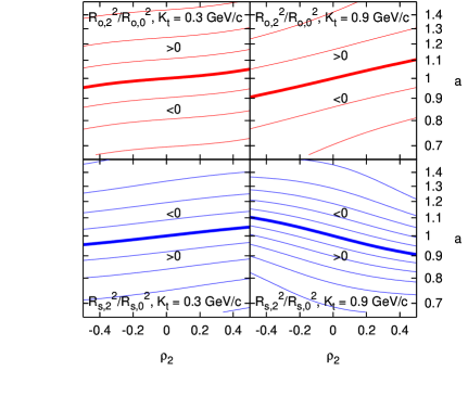
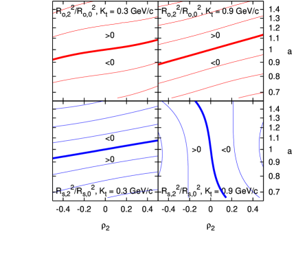
Model 1 Model 2

Figure 3: Normalised oscillation amplitudes $R_{o,2}^{2}/R_{o,0}^{2}$ (upper row) and $R_{s,2}^{2}/R_{s,0}^{2}$ (lower rows) as functions of $a$ and $\rho_{2}$ calculated for $T=0.1\,\mbox{GeV},\,\rho_{0}=0.88,\,R=9.41\,\mbox{fm},\,\tau_{0}=9\,\mbox{fm}/c,\,\Delta\tau=1\,\mbox{fm}/c$ (see asym for definitions of all parameters). Left columns show results for $K_{T}=0.3\,\mbox{GeV}/c$, right columns correspond to $K_{T}=0.9\,\mbox{GeV}/c$. Thickest lines show where the second-order oscillation terms vanish, other contours are set in steps of 0.1.

From Figure 3 we conclude that the azimuthal oscillations of the HBT correlation radii are mainly shaped by the spatial anisotropy parameter $a$. Dependence on flow anisotropy is weaker, with the only exception of $R_{s}^{2}$ at high $K_{t}$ in Model 2 which is determined mainly by flow. This confirms the statement that the azimuthal dependence of correlation radii follows mainly the spatial anisotropy, especially at low $K_{t}$. This has been shown here in framework of two models. It would be natural to expect this behaviour to be valid in general. It can be spoilt by very strong flow gradients which differ by much in in-plane and out-of-plane directions. A questions arises, however, whether large enough difference of the flow gradients is realistic.

The two investigated models exhibit similar dependence on the spatial anisotropy parameter $a$ when focusing on the oscillation of HBT radii. Recall, however, that they were related by transformation $a\to a^{-1}$ when reproducing the same $v_{2}$. Therefore, two different models which both reproduce $v_{2}$ measurement will behave differently when fitting the azimuthal dependence of HBT radii. This is illustrated in Figure 4.

Figure 4: Comparison of the dependence of $R_{o}^{2}$ and $R_{s}^{2}$ on azimuthal angle $\phi$ with the data measured by STAR collaboration (Au+Au at 200 $A$GeV, centrality class 20–30%) STARdata . The curves and data points correspond from top to bottom to $K_{T}=0.2,\,0.3,\,0.4,\,0.52\,\mbox{GeV}/c$. Parameters of the models are: $T=0.12\,\mbox{GeV},\,\rho_{0}=0.99,\,\rho_{2}=0.035,\,R=9.41\,\mbox{fm},\,\tau_{0}=5.02\,\mbox{fm}/c,\,\Delta\tau=2.9\,\mbox{fm}/c$, and $a=0.946$ (Model 1) or $a=1.057$ (Model 2). Both models were tuned to fit $v_{2}(p_{T})$ Tomasik:2004bp .

Both models used in this figure fit measured the $v_{2}$ for pions and protons well. However, while Model 1 reproduces the RHIC data qualitatively well, Model 2 leads to the phase of oscillation just opposite to data STARdata .

Thus we conclude that among the two models used in this study, Model 1 seems to correspond to RHIC data, whereas Model 2 is clearly ruled out. This does not disqualify it, however, from future applications at the LHC where possibly longer lived fireballs could be produced which will develop a different transverse flow pattern.

5 Conclusions

It has been demonstrated analytically that one cannot disentangle spatial and flow anisotropy of the fireball just from a measurement of $v_{2}$. I also demonstrated that, at least for two classes of models, the azimuthal dependence of correlation radii reflects the type of spatial anisotropy the source actually exhibits.

Thus I can propose the following (schematic) procedure for disentangling $a$ and $\rho_{2}$: first measure the azimuthal dependence of HBT radii and determine the spatial anisotropy $a$. Then, with that $a$ try to reproduce $v_{2}$ for more species. Since for different species $a$ and $\rho_{2}$ are correlated in different ways, this should lead to unique pair of the anisotropy parameters.

6 Acknowledgements

This research and presentation were supported by a Marie Curie Intra-European Fellowship within the 6th European Community Framework Programme.

References

- (1) S. Voloshin and Y. Zhang, Z. Phys. C 70, 665 (1996).
- (2) C. Adler at al. [STAR Collaboration], Phys. Rev. Lett. 87, 182301 (2001).
- (3) U. Heinz and P.F. Kolb, Phys. Lett. B 542, 216 (2002).
- (4) B. Tomášik, Acta Physica Polonica B 36, 2087 (2005).
- (5) F. Retière and M.A. Lisa, Phys. Rev. C 70, 044907 (2004).
- (6) U. Heinz, A. Hummel, M. A. Lisa and U. A. Wiedemann, Phys. Rev. C 66, 044903 (2002).
- (7) B. Tomášik and U. A. Wiedemann, “Central and non-central HBT from AGS to RHIC”, in Quark Gluon Plasma 3, edited by R.C. Hwa and X.N. Wang, World Scientific, Singapore, 2004, pp. 715-777, [arXiv:hep-ph/0210250].
- (8) J. Adams et al. [STAR Collaboration], Phys. Rev. Lett. 93, 012301 (2004).
- (9) B. Tomášik, Nucl. Phys. A 749, 209 (2005).