Effective Field Theory of Nucleon-Nucleon Scattering
on Large Discrete Lattices

Abstract

Nuclear effective field theory is applied to the effective range expansion of S-wave nucleon-nucleon scattering on a discrete lattice. Lattice regularization is demonstrated to yield the effective range expansion in the same way as in the usual continuous open space. The relation between the effective range parameters and the potential parameters is presented in the limit of a large lattice.

I Introduction

In the last several years nuclear effective field theory (EFT) has been applied extensively to low-energy nucleon-nucleon interactions and to few-nucleon systems review . At energies below 1 GeV or so, quantum chromodynamics (QCD) reduces to a hadronic theory containing all interactions allowed by the symmetries of the theory. At the very lowest energies, the interactions are of contact type among nucleons, with arbitrary number of derivatives. For the two-nucleon system, the nuclear EFT has established a concrete systematic foundation for the traditional description represented by the effective range expansion (ERE), even with large S-wave scattering lengths generated by bound or nearly bound states vankolck ; ksw ; gegelia . In systems with more than two nucleons few-body contact forces are present —a three-body force appears already in leading order— and the EFT provides a well-defined, successful extension of the ERE three ; four . At higher energies, pions need to be accounted for explicitly in the theory. In this case, the EFT goes beyond the ERE even in the two-nucleon system, albeit at the cost of a much more complicated renormalization structure review .

Once the leading few-body interactions are determined from few-body systems, the main goal of the EFT program is to predict the structure of larger nuclei. Before tackling heavy nuclei, one would like to be able to predict the properties of infinite nuclear matter. This requires a method of solution whose errors are not larger than EFT truncation errors. A few years ago it was suggested that this could be achieved by putting nucleons on a spatial lattice and using Monte Carlo methods to compute the partition function mksv . In this first, exploratory investigation we considered two-nucleon contact interactions only, with parameters adjusted to nuclear matter properties. Subsequently, works have appeared that extend this approach in various directions chen ; shailesh ; ASK ; deanlee1 ; deanlee2 ; deanlee3 ; aurel . As yet, however, a full application of EFT to nuclear matter has not been carried out. In this work we take the first step toward this goal by examining the effective range expansion of nucleon-nucleon scattering on a discrete lattice. The extension of this work to the determination of thermal properties of neutron matter from parameters from few-body physics is currently underway AS .

As in any field theory, the parameters that appear in the EFT Lagrangian or Hamiltonian are not directly observable, since the separation between them and the high-momentum components of loops is arbitrary. This separation is the regularization procedure, such as momentum cutoff and dimensional. Because the separation is arbitrary, relations among observables should not depend on the regularization scheme. The relation between EFT parameters and observables, on the other hand, does depend on the regularization, and some regularization schemes are more convenient to apply than others. The program of predicting many-body properties from few-body physics requires that the relation between parameters and observables be known within the regularization scheme employed in the solution of the many-body problem. Placing nucleons in a lattice is a choice of a regularization scheme.

In this work, we examine lattice regularization for the effective field theory on a discrete three-dimensional cubic lattice of a large size. The special aspect associated with the use of a lattice is that the nucleons are interacting in a closed space, different from scattering of nucleons in the open space. On this issue, the method of Lüscher luescher is well known in lattice QCD, and it has been also studied for the nucleon-nucleon interaction beane04 , especially on the treatment of the scattering lengths larger than the lattice size. These works examine effects of finite-volume lattice space in the limit of vanishing lattice spacing, that is, in the continuum limit. Here, we focus on effects of the finite lattice spacing in the limit of large lattice volume.

Our objective is to determine the parameters of the two-body interaction on the lattice from known phase shifts. We illustrate the method in the case of sufficiently low energies, when the phase shifts can be represented by the ERE parameters. The method is similar to the continuum case considered in Ref. vankolck , and follows a preliminary attempt involving one of us (R.S.) several years ago m-s . An earlier, related work can be found in Ref. dy . Our results can be applied to the two-nucleon system at low energies, and the interaction parameters thus determined are to be used for the many-body Monte Carlo calculation of Ref. AS . In principle, the whole framework could be used at higher energies, densities and temperatures, once pion exchange is included explicitly.

The cutoff or renormalization scale is kept at finite values, and so is the corresponding lattice spacing. As the thermal properties should be examined at the thermal or infinite-volume limit, the lattice results needed are at the limit of large lattice space. This is usually achieved by performing many-body Monte Carlo calculations with various lattice sizes, followed by applying the method of finite-size scaling fss . Upon application of the method, there is no need to consider explicit dependence on the lattice size in our potential parameters. Determination of the parameters is greatly simplified at the limit of large space size. In fact, we find that the basic algebra is the same as that in free space, apart from the use of the reaction (K) matrix instead of the standard scattering (T) matrix.

The paper is organized as follows. We briefly discuss the K matrix as a description of the two-body interaction in a closed space in Sect. II. In Sect. III, the relation between the effective range parameters and the potential parameters is obtained by the use of a diagrammatic expansion of the K matrix. An alternative derivation by the direct use of the wave function is given in App. A. The case of a large, discrete lattice is treated in Sect. IV. An elaboration of the mathematical treatment of the Green’s function in this case is given in App. B. A brief discussion of our results in comparison with Lüscher’s method and some other concluding remarks are presented in Sect. V.

II K (Reaction) matrix in closed space

Our method is based on essentially the same scattering formalism as the well-known Lüscher method luescher is. We find that the use of the reaction, or K, matrix (also termed the reactance matrix, or R, matrix) newton ; gw , whose language is more familiar to the nuclear physics community, greatly simplifies the formalism.

We consider two particles of mass $M$ interacting through a potential $V({{\bm{r}}})$. The wave function for the relative motion, $\psi_{{\bm{p}}}({{\bm{r}}})$, satisfies the Schrödinger equation,

$$-(\nabla^{2}/M)\psi_{{\bm{p}}}({{\bm{r}}})+V({\bm{r}})\psi_{{\bm{p}}}({{\bm{r}}})=E_{p}\psi_{{\bm{p}}}({{\bm{r}}})\;,$$ (1)

with $E_{p}={{\bm{p}}}^{2}/M=p^{2}/M$ ($p\equiv|{{\bm{p}}}|$). As Eq. (1) is of second order, $\psi_{{\bm{p}}}({{\bm{r}}})$ can be set to describe the physical state of interest as a combination of two independent solutions by appropriately choosing boundary conditions. The standard choice of boundary condition is that the wave function has, apart from the incident plane wave, an outgoing wave with the asymptotic form $\exp(ipr)/r$, or (though less popular) an incoming wave with $\exp(-ipr)/r$, either one providing the T matrix, the usual scattering amplitude. Another choice is for the wave function to have a standing-wave form, a combination of the two asymptotic forms. More explicitly, the wave function in the $\ell$-th angular momentum state has the asymptotic form:

$$R_{\ell}(pr)\rightarrow j_{\ell}(pr)-\frac{1}{2}\left(S_{\ell}(p)-1\right)h^{(1)}_{\ell}(pr)$$

for the T matrix, or

$$R_{\ell}(pr)\rightarrow j_{\ell}(pr)-pK_{\ell}(p)n_{\ell}(pr)$$

for the K matrix. Here, $K_{\ell}(p)\equiv-(i/p)(S_{\ell}(p)-1)/(S_{\ell}(p)+1)$ is the K matrix, and $S_{\ell}(p)=e^{2i\delta_{\ell}}$ is the S matrix expressed in terms of the corresponding phase shift $\delta_{\ell}$. $h^{(1)}_{\ell}(pr)=j_{\ell}(pr)+in_{\ell}(pr)$ is the spherical Bessel function of the third kind abm . Note that the first term of the spherical Bessel function $j_{\ell}(pr)$ in the above equations forms the incident plane wave. From $R_{\ell}(pr)$, the total wave functions is constructed as

$$\psi_{{\bm{p}}}({{\bm{r}}})=\sum_{\ell=0}^{\infty}(2\ell+1)i^{\ell}R_{\ell}(pr)P_{\ell}(\cos\theta)\;,$$ (2)

where $P_{\ell}(\cos\theta)$ is the Legendre polynomial with $\theta$ the angle between ${{\bm{p}}}$ and ${{\bm{r}}}$.

Clearly, the choices of the outgoing and incoming boundary conditions are unsuited for the description of two particles interacting in a closed space. The choice of the standing-wave boundary condition can be made by requiring $V({\bm{r}})$ and $\psi_{{\bm{p}}}({{\bm{r}}})$ to satisfy periodic conditions, such as those that make a cubic box of size $L\times L\times L$ into a torus,

$$V({{\bm{r}}}+{{\bm{n}}}L) = V({{\bm{r}}})\;,$$

$$\psi_{{\bm{p}}}({{\bm{r}}}+{{\bm{n}}}L) = \psi_{{\bm{p}}}({{\bm{r}}})\;,$$ (3)

where ${\bm{n}}$ is an integer vector with its components covering a set of all integer values. Equation (3) restricts the allowed values of $\{{\bm{p}}\}$ to be discrete. In fact, the Green’s function satisfying Eq. (3) with the standing-wave boundary condition is written as

$$G_{\rm P}({\bm{p}},{{\bm{r}}}-{{\bm{r}}^{\prime}})\equiv\frac{1}{L^{3}}\sum_{{{\bm{p}}^{\prime}}(\neq{{\bm{p}}})}\frac{\phi_{{\bm{p}}^{\prime}}({{\bm{r}}})\phi^{*}_{{\bm{p}}^{\prime}}({{\bm{r}}^{\prime}})}{E_{p}-E_{p^{\prime}}}\;,$$ (4)

and obeys

$$[-\nabla^{2}/M-{{\bm{p}}}^{2}/M]G_{\rm P}({\bm{p}},{{\bm{r}}}-{{\bm{r}}^{\prime}})=-\frac{1}{L^{3}}\sum_{{{\bm{p}}^{\prime}}(\neq{{\bm{p}}})}\phi_{{\bm{p}}^{\prime}}({{\bm{r}}})\phi^{*}_{{\bm{p}}^{\prime}}({{\bm{r}}^{\prime}})=-\delta({\bm{r}}^{\prime}-{\bm{r}})+\phi_{{\bm{p}}}({{\bm{r}}})\phi^{*}_{{\bm{p}}}({{\bm{r}}^{\prime}})\;,$$ (5)

where $\phi_{{\bm{p}}}({{\bm{r}}})\equiv{\exp}(i{{\bm{p}}}\cdot{{\bm{r}}})$. Here, ${\bm{p}}^{\prime}=2\pi{\bm{n}}/L$ is the undisturbed (by $V({\bm{r}})$) momentum, while $\{{\bm{p}}\}$ forms a discrete set of eigenmomenta in the closed space, which are determined through a decomposition of the above Green’s function as elaborated in Ref. luescher .

In this work, we examine the large-lattice limit by letting $L\rightarrow\infty$. In this limit, the periodic condition of Eq. (3) becomes ineffective and imposes no special condition, ${\bm{p}}$ becoming a continuous spectrum bounded by the inverse of the finite lattice spacing. The ${\bm{p}}^{\prime}$ sum becomes an integral,

$$\frac{1}{L^{3}}\sum_{{{\bm{p}}^{\prime}}(\neq{{\bm{p}}})}\rightarrow\wp\int\frac{d^{3}p^{\prime}}{(2\pi)^{3}}\;,$$ (6)

where $\wp$ stands for the principal value of the integral, excluding the contribution from ${\bm{p}}^{\prime}={\bm{p}}$. The range of the integration in Eq. (6) is also restricted by the inverse of the finite lattice spacing.

Our method of using the K matrix is equally applicable to both a large, closed space and (open) free space. In fact the formalism and basic algebra are the same. The K matrix $K({{\bm{p}}^{\prime}},{{\bm{p}}})$ is defined gw in terms of $\psi_{{\bm{p}}}({{\bm{r}}})$ with the boundary condition (2) as

$$K({{\bm{p}}^{\prime}},{{\bm{p}}})\equiv\int d^{3}r\phi^{*}_{{\bm{p}}^{\prime}}({{\bm{r}}})V({\bm{r}})\psi_{{\bm{p}}}({{\bm{r}}})\;,$$ (7)

and it satisfies the integral equation

$$K({{\bm{p}}^{\prime}},{{\bm{p}}})=V({{\bm{p}}^{\prime}},{{\bm{p}}})+\wp\int\frac{d^{3}p^{\prime\prime}}{(2\pi)^{3}}V({{\bm{p}}^{\prime}},{\bm{p}^{\prime\prime}})\bar{G}({\bm{p}^{\prime\prime}};{{\bm{p}}})K({\bm{p}^{\prime\prime}},{{\bm{p}}})\;.$$ (8)

Here, $V({{\bm{p}}^{\prime}},{{\bm{p}}})$ and $\bar{G}({{\bm{p}}^{\prime}},{{\bm{p}}})$ are related to $V({\bm{r}})$ and $G_{\rm P}({\bm{p}},{{\bm{r}}}-{{\bm{r}}^{\prime}})$ as

$$V({{\bm{p}}^{\prime}},{{\bm{p}}}) = \int d^{3}r{\phi^{*}_{{\bm{p}}^{\prime}}({{\bm{r}}})V({\bm{r}})\phi_{{\bm{p}}}({{\bm{r}}})}\;,$$ (9)

$$(2\pi)^{3}\delta^{3}({\bm{p}}^{\prime\prime}-{\bm{p}}^{\prime})\wp\bar{G}({{\bm{p}}^{\prime}};{{\bm{p}}}) = \int d^{3}r\int d^{3}r^{\prime}{\phi^{*}_{{\bm{p}}^{\prime\prime}}({{\bm{r}}})G_{\rm P}({\bm{p}},{{\bm{r}}}-{{\bm{r}}^{\prime}})\phi_{{\bm{p}}^{\prime}}({{\bm{r}}^{\prime}})}$$ (10)

$$= (2\pi)^{3}\delta^{3}({\bm{p}}^{\prime\prime}-{\bm{p}}^{\prime})\wp\frac{M}{p^{2}-{p^{\prime}}^{2}}\;,$$

respectively. Note $\wp$ implies ${\bm{p}}\neq{\bm{p}}^{\prime}$ in this case.

Equation (8) is the same integral equation that the standard T matrix $T({{\bm{p}}^{\prime}},{{\bm{p}}})$ satisfies for scattering in free space, except for the Green’s function satisfying the standing-wave boundary condition. Because the two equations are of the same structure, the diagrammatic expansions generated from them, as expansions in terms of $V({\bm{p}}^{\prime},{\bm{p}})$, are also of the same structure, apart from the presence of the $+ip$ term appearing in the T matrix. This term comes from the ${\bm{p}}^{\prime}={\bm{p}}$ contribution that is included in the T-matrix Green’s function (usually denoted as $G^{(+)}({\bm{p}^{\prime}},{{\bm{p}}})$ for the outgoing boundary condition). The $+ip$ term is vital for the T matrix to satisfy the unitarity condition, while the term is not present in the K matrix, as the K matrix is Hermitian.

Successive substitution of Eq. (9) into Eq. (8) yields a diagrammatic expansion of the on-shell K matrix. For getting the expansion, however, we must regulate Green’s function and related (momentum-space) integrals, as discussed in Sect. III.

$K({{\bm{p}}^{\prime}},{{\bm{p}}})$ is expanded in angular momentum states,

$$K({{\bm{p}}^{\prime}},{{\bm{p}}})=-\frac{4\pi}{M}\sum_{\ell}(2\ell+1)P_{\ell}(\hat{{\bm{p}}}\,^{\prime}\cdot\hat{{\bm{p}}})K_{\ell}(p^{\prime},p)\;,$$ (11)

where $\hat{{\bm{p}}}\,^{\prime}$ and $\hat{{\bm{p}}}$ are unit momentum vectors. The coefficient $(-4\pi/M)$ is introduced so that the on-shell $K_{\ell}(p,p)$ is expressed in terms of the $\ell$-th phase shift $\delta_{\ell}$ as

$$K_{\ell}(p,p)\equiv K_{\ell}(p)=\frac{1}{p}\tan\delta_{\ell}(p)\;.$$ (12)

$K_{\ell}(p)$ is a real function of $p^{2}$ that is known to be analytic around $p=0$, so it can be written as the effective range expansion with a convergence radius of $p^{2}\approx 1/(2R)^{2}$ in the case of scattering from a potential of the range $R$ newton . The S-wave expansion relevant to this work is

$$K_{0}^{-1}(p)=p\cot\delta_{0}(p)=-\frac{1}{a_{0}}+\frac{1}{2}r_{0}p^{2}+\mathcal{O}(p^{4})\;,$$ (13)

where $a_{0}$ and $r_{0}$ are the s-wave scattering length and the effective range, respectively.

III Relation between effective-range and potential parameters using K matrix

In this section, we express the effective-range parameters in terms of the potential parameters using the K matrix without specifying the regularization method. As noted in Sect. II, our method of the K matrix is equally applicable to a large, closed space and to (open) free space. The algebra is the same except for the details associated with regularization. Without specifying the regularization method, we can then compare our method to the previous works based on diagrammatic expansions of the T matrix, which use different regularization methods vankolck ; ksw ; gegelia . In order to solidify the comparison, in App. A we also show the derivation of the same results using the wave function, instead of the diagrammatic expansion, starting from the definition of the K matrix, Eq. (7). The explicit case of the lattice regularization (for a large, closed space) will be discussed in Sect. IV.

We consider the case where the two particles interact through a short-range potential, which is expressed in the form of effective field theory, consisting of a combination of $\delta^{3}({\bm{r}})$ and powers of the nucleon momentum (square) ${{\bm{p}}}^{2}$,

$$V({{\bm{r}}})=c_{0}(\Lambda)\delta^{3}({{\bm{r}}})-c_{2}(\Lambda)[\nabla^{2}\delta^{3}({{\bm{r}}})+\delta^{3}({{\bm{r}}})\nabla^{2}]+\ldots\;,$$ (14)

where the parameters $c_{0}$, $c_{2}$, etc. depend on the cutoff scale, $\Lambda$. (In the case of a periodic condition (3), $\delta^{3}({\bm{r}})$ in $V({\bm{r}})$ of Eq. (14) is to be replaced by a sum over ${\bm{n}}$ of $\delta^{3}({{\bm{r}}}+{{\bm{n}}}L)$.) In momentum space,

$$V({{\bm{p}}^{\prime}},{{\bm{p}}})=c_{0}+c_{2}(p^{2}+{p^{\prime}}^{2})+\ldots$$ (15)

Here we show explicitly only the leading terms in the potential for the case of interest: low-energy phenomena dominated by the S-wave interaction. We do not show explicitly higher-order terms such as the P-wave term $\loarrow{\nabla}\cdot\roarrow{\nabla}$ or relativistic corrections proportional to ${{\bm{p}}^{4}}$. A more complete discussion of the various terms can be found in Ref. vankolck . The potential (14) is generated by removing from the theory other degrees of freedom, whose effects are now subsumed in $c_{0}$, $c_{2}$, and higher-order counterterms. For example, in the case the particles are nucleons, pion-interaction effects can be effectively included in contact interactions for $|{\bm{p}}|<m_{\pi}/2$, where $m_{\pi}$ is the pion mass.

The potential (15) is singular, in the sense that it requires that the problem be regulated. For example, an integral of the Green’s function of Eq. (10) becomes

$$\wp\int\frac{d^{3}{\bm{p}^{\prime}}}{(2\pi)^{3}}\bar{G}({\bm{p}}^{\prime};{\bm{p}})\rightarrow M\wp\int\frac{d^{3}{\bm{p}^{\prime}}}{(2\pi)^{3}}\frac{F({\bm{p}^{\prime}}^{2}/\Lambda^{2})}{p^{2}-{\bm{p}^{\prime}}^{2}}\equiv I_{0}(p,\Lambda)\;$$ (16)

by the use of a multiplicative regulator $F(x^{2})$, which satisfies $\lim_{x\to\infty}F(x^{2})=0$ and $\lim_{x\to 0}F(x^{2})=1$.

For the sake of comparison with other regularization methods, let us take $F(x^{2})$ to be simply an integrable function of $x^{2}$. We then have

$$I_{0}(p,\Lambda) = -\frac{M}{2\pi^{2}}\left[\int_{0}^{\infty}dp^{\prime}F({p^{\prime}}^{2}/\Lambda^{2})-p^{2}\cdot\wp\int_{0}^{\infty}dp^{\prime}\frac{F(p^{\prime 2}/\Lambda^{2})}{p^{2}-p^{\prime 2}}\right]$$ (17)

$$\equiv -\frac{M}{2\pi^{2}}\left[L_{1}(\Lambda)+\frac{p^{2}}{\Lambda}R((p/\Lambda)^{2})\right]\;.$$

Here, $L_{1}(\Lambda)$ is

$$L_{1}(\Lambda)\equiv\int_{0}^{\infty}dp^{\prime}F(p^{\prime 2}/\Lambda^{2})\equiv\theta_{1}\Lambda\;,$$ (18)

with

$$\theta_{1}\equiv\int_{0}^{\infty}dxF(x^{2})\;,$$ (19)

and $R(x^{2})$,

$$R(x^{2})=\wp\int_{0}^{\infty}dx^{\prime}\frac{F({x^{\prime}}^{2})}{{x^{\prime}}^{2}-x^{2}}\;.$$ (20)

We expect $\theta_{1}=\mathcal{O}(1)$, but the exact value depends on the regulator. $R(x^{2})$ is also a regulator-dependent function. For a sharp cutoff regulator $F(x^{2})=\theta(1-x)\theta(x)$, we have

$$\theta_{1}=1\;\;{\rm and}\;\;R(x^{2})=\frac{1}{2x}\ell n((1-x)/(1+x))=1+\frac{1}{3}x^{2}+\ldots$$

Another regulated integral that appears is

$$I_{2}(p,\Lambda) = \wp\int\frac{d^{3}{\bm{p}^{\prime}}}{(2\pi)^{3}}\frac{{\bm{p}^{\prime}}^{2}F({\bm{p}}^{\prime 2}/\Lambda^{2})}{E_{\bm{p}}-E_{\bm{p}^{\prime}}}$$ (21)

$$= -\frac{M}{2\pi^{2}}L_{3}(\Lambda)+p^{2}I_{0}(p,\Lambda)\;,$$

with

$$L_{3}(\Lambda)\equiv 2\pi^{2}\int\frac{d^{3}{\bm{p}^{\prime}}}{(2\pi)^{3}}F({\bm{p}}^{\prime 2}/\Lambda^{2})\equiv\theta_{3}\Lambda^{3}\;.$$ (22)

For the sharp cutoff regulator,

$$\theta_{3}=\frac{1}{3}\;.$$ (23)

We can define analogous integrals $I_{2n}$, which satisfy recurrence relations,

$$I_{2n}(p,\Lambda) \equiv \wp\int\frac{d^{3}p^{\prime}}{(2\pi)^{3}}\frac{p^{\prime 2n}F(p^{\prime 2}/\Lambda^{2})}{E_{\bm{p}}-E_{\bm{p}^{\prime}}}$$ (24)

$$= -\frac{M}{2\pi^{2}}L_{2n+1}(\Lambda)+p^{2}I_{2n-2}(p,\Lambda)\;,$$

with

$$L_{2n+1}(\Lambda)\equiv 2\pi^{2}\int\frac{d^{3}p^{\prime}}{(2\pi)^{3}}{p^{\prime}}^{2n-2}F(p^{\prime 2}/\Lambda^{2})\;,$$ (25)

and thus

$$I_{2n}=-\frac{M}{2\pi^{2}}\left[\sum_{i=0}^{n}p^{2i}L_{2(n-i)+1}(\Lambda)+\frac{p^{2(n+1)}}{\Lambda}R(p^{2}/\Lambda^{2})\right]\;.$$ (26)

The diagrammatic expansion of $K({{\bm{p}}},{{\bm{p}}})$ is depicted in Fig. 1. In the case of large S-wave scattering length $a_{0}$, $c_{0}(\Lambda)I_{0}(p,\Lambda)$ is close to unity and diagrams of all orders in $c_{0}(\Lambda)$ must be included. We denote by $K_{1}$ the sum of the $c_{0}(\Lambda)$ contributions,

$$K_{1}\equiv c_{0}(\Lambda)+c_{0}(\Lambda)I_{0}(p,\Lambda)c_{0}(\Lambda)+c_{0}(\Lambda)I_{0}(p,\Lambda)c_{0}(\Lambda)I_{0}(p,\Lambda)c_{0}(\Lambda)+\ldots$$ (27)

On the other hand, $c_{2}(\Lambda)$ should be treated perturbatively vankolck . We denote the sets of diagrams with one insertion of $c_{2}(\Lambda)$ by $K_{2},K_{21},$ and $K_{121}$ if they have, respectively, no $c_{0}(\Lambda)$ factors, $c_{0}(\Lambda)$ factors either before or after the $c_{2}(\Lambda)$ insertion, and $c_{0}(\Lambda)$ factors both before and after the $c_{2}(\Lambda)$ insertion. The procedure can easily be extended to higher orders. We have

$$-\frac{4\pi}{M}K_{0}(p) = K_{1}+K_{2}+2\cdot K_{21}+K_{121}+\mathcal{O}(c_{2}^{2},p^{4})\;.$$ (28)

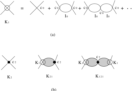
Figure 1: Diagrammatic representation of $K_{1},K_{2},K_{21}$, and $K_{121}$. The upper figure (a) depicts $K_{1}$ as a sum of the iteration of $c_{0}$, Eq. (27), with a crossing point as $c_{0}$. The open bubble is the regulated Green’s function $I_{0}$. The lower figure (b) shows $K_{2},K_{21}$, and $K_{121}$ as in Eq. (29), with an open circled vertex as $K_{1}$ and with a dot vertex as $c_{2}$. The shaded bubble is a regulated Green’s function weighted with vertex momenta, $I_{2}$.

After some algebra, we find (suppressing the explicit showing of the $p$ and $\Lambda$ dependence for a while)

$$K_{2} = 2p^{2}c_{2}\;,$$

$$K_{21} = K_{1}\cdot c_{2}(I_{2}+p^{2}I_{0})\;,$$

$$K_{121} = 2K_{1}^{2}c_{2}I_{0}I_{2}\;.$$ (29)

Because

$$2\cdot K_{21}+K_{121}=2K_{1}\frac{c_{2}}{c_{0}}(I_{2}K_{1}+c_{0}p^{2}I_{0})\;,$$

we obtain for $K_{0}(p)$,

$$-\frac{M}{4\pi}K_{0}^{-1}(p) = K_{1}^{-1}\frac{1}{1+2(c_{2}/c_{0})(p^{2}+K_{1}I_{2})}+\mathcal{O}(c_{2}^{2},p^{4})$$ (30)

$$= \frac{1}{c_{0}}+\frac{M}{2\pi^{2}}\left[L_{1}+\frac{p^{2}}{\Lambda}R((p/\Lambda)^{2})\right]-2\frac{c_{2}}{c_{0}}\left[\frac{p^{2}}{c_{0}}-\frac{M}{2\pi^{2}}L_{3}\right]+\mathcal{O}(c_{2}^{2},p^{4})$$

$$= \frac{1}{c_{0}}+\frac{M}{2\pi^{2}}\left(L_{1}+2\frac{c_{2}}{c_{0}}L_{3}\right)+\left(\frac{M}{2\pi^{2}\Lambda}R(0)-2\frac{c_{2}}{c_{0}^{2}}\right)p^{2}+\mathcal{O}(c_{2}^{2},p^{4})\;.$$

We emphasize that in this derivation, $1-c_{0}I_{0}$, not $c_{0}$, is treated perturbatively. We add here a note that Eq. (30) can be also written as

$$-\frac{4\pi}{M}K_{0}(p)=\frac{c_{0}+2c_{2}p^{2}}{1-(c_{0}I_{0}+2c_{2}I_{2})}+\mathcal{O}(c_{2}^{2},p^{4})\;,$$ (31)

with the understanding that $1-c_{0}I_{0}$ (but not $c_{0}$) and $c_{2}$ are treated perturbatively. Up to the $\mathcal{O}(c_{2})$ order, Eq. (31) has the same structure as that of $K_{0}(p)$ obtained ksw by the power divergence subtraction (PDS) scheme (with their definition of $c_{2}$ being half of ours).

The S-wave scattering length and effective range are thus expressed as

$$\frac{M}{4\pi}\frac{1}{a_{0}} = \frac{1}{c_{0}(\Lambda)}+\frac{M}{2\pi^{2}}\left(L_{1}(\Lambda)+2\frac{c_{2}(\Lambda)}{c_{0}(\Lambda)}L_{3}(\Lambda)\right)+\ldots$$

$$\frac{M}{16\pi}r_{0} = \frac{c_{2}(\Lambda)}{c_{0}^{2}(\Lambda)}-\frac{M}{4\pi^{2}}\frac{1}{\Lambda}R(0)+\ldots\;,$$ (32)

where terms up to next-to-leading order are explicitly shown. Equation (32) is in agreement with Ref. vankolck . Note that terms beyond this order must include potential terms of $p^{4}$ and higher.

In this case of a large S-wave scattering length, the dimensionless parameter $c_{0}(\Lambda)\theta_{1}\Lambda M$ is near its (unstable) fixed point $-2\pi^{2}$ weinberg ,

$$c_{0}(\Lambda)=\frac{4\pi}{M}\left[\frac{1}{a_{0}}-\frac{2\theta_{1}\Lambda}{\pi}\right]^{-1}+\ldots\approx-\frac{2\pi^{2}}{\theta_{1}M\Lambda}\;,$$ (33)

while it flows to the trivial fixed point at the zero value for $\pi/(2\theta_{1}a_{0})\gg\Lambda\rightarrow 0$ birse . This observation is consistent with the counting rule that we have followed: Since our non-relativistic Hamiltonian is a momentum expansion based on power-counting rules vankolck , it is an expansion about the trivial point. As the leading term of the expansion about $p^{2}=0$, the delta-function potential has to be treated nonperturbatively in order to describe the physics near the unstable fixed point, away from the trivial one.

IV Closed, large, discrete lattice

We now examine the effective range expansion on a closed, large, discrete lattice. We consider a spatial lattice that is simply cubic with lattice spacing $a$ and volume $L^{3}=(aN)^{3}$, in the limit of $N\rightarrow\infty$.

The coordinate is discretized in units of $a$,

$${\bm{r}}\rightarrow a{\bm{n}}\;,$$ (34)

where ${\bm{n}}=\sum_{i}n_{i}\hat{\bm{r}}_{i}$ is again a vector with integer components $n_{i}$ along the directions given by the Cartesian unit vectors $\hat{\bm{r}}_{i}$, $i=1,2,3$. Since

$$\int d^{3}r\rightarrow\sum_{\bm{n}}a^{3}\;,$$ (35)

we have also

$$\delta^{3}({\bm{r}})\rightarrow\frac{1}{a^{3}}\delta_{{\bm{n}},0}\;.$$ (36)

The range of momenta is limited to the first Brillouin zone,

$$-\frac{\pi}{a}\leq p_{i}\leq\frac{\pi}{a}\;,$$ (37)

for each momentum component $i$. In the limit $N\to\infty$ the momentum is continuum in this interval. The wave functions in coordinate and momentum spaces are related by

$$\psi(a{\bm{n}})=\int^{\pi/a}_{-\pi/a}\int^{\pi/a}_{-\pi/a}\int^{\pi/a}_{-\pi/a}\frac{dp_{1}dp_{2}dp_{3}}{(2\pi)^{3}}\tilde{\psi}({\bm{p}})e^{ia{\bm{n}}\cdot{\bm{p}}}\;,$$

which is seen to satisfy the required periodicity even for a finite ${\bm{n}}$, Eq. (3) with Eq. (34).

When the standard four-point difference formula is used, the kinetic-energy operator is expressed on the cubic spatial lattice as

$$-\nabla^{2}\psi_{{\bm{p}}}({{\bm{r}}}) \rightarrow -\sum_{i=1}^{3}\frac{1}{a^{2}}\left\{\psi\left((\bm{n}+\hat{\bm{r}}_{i})a\right)+\psi\left((\bm{n}-\hat{\bm{r}}_{i})a\right)-2\psi(a\bm{n})\right\}$$ (38)

$$= \int^{\pi/a}_{-\pi/a}\int^{\pi/a}_{-\pi/a}\int^{\pi/a}_{-\pi/a}\frac{dp_{1}dp_{2}dp_{3}}{(2\pi)^{3}}\tilde{\psi}({\bm{p}})e^{i{\bm{n}}\cdot{\bm{p}}}\frac{1}{a^{2}}P({\bm{p}})\;.$$

That is, as an operator in the spatial space, ${{\bm{p}}}^{2}$ is represented as

$${{\bm{p}}}^{2}\rightarrow\frac{1}{a^{2}}P({\bm{p}})\equiv\frac{2}{a^{2}}\sum_{i=1}^{3}(1-\cos(ap_{i}))\;.$$ (39)

$P({\bm{p}})/a^{2}$ becomes ${{\bm{p}}}^{2}$ in the continuum limit $a\rightarrow 0$, while for a finite $a$, we have

$$0\leq\frac{1}{a^{2}}P({\bm{p}})\leq\frac{12}{a^{2}}\;.$$ (40)

$P({\bm{p}})=0$ occurs only when ${\bm{p}}=0$, and thus we have no problem of fermion doubling. Note that Eq. (39) leads to the formal operator expression for the regulator,

$$F\left(\frac{a^{2}p^{\prime 2}}{\pi^{2}}\right)=\left(\frac{a}{\pi}\right)^{2}\int^{\pi/a}_{-\pi/a}\int^{\pi/a}_{-\pi/a}\int^{\pi/a}_{-\pi/a}\frac{dp^{\prime\prime}_{1}dp^{\prime\prime}_{2}dp^{\prime\prime}_{3}}{(2\pi)^{3}}\;\delta\left(\left(\frac{ap^{\prime}}{\pi}\right)^{2}-\frac{2}{\pi^{2}}\sum_{i=1}^{3}\left[1-\cos\left(ap^{\prime\prime}_{i}\right)\right]\right)\;,$$ (41)

showing explicitly that a cubic spatial symmetry is now imposed. This suggests the identification

$$\frac{\pi}{a}\sim\Lambda\;.$$ (42)

We then write

$$I_{0}(p,a) \equiv -\frac{M}{2a}\frac{1}{(2\pi)^{3}}\wp\int^{\pi}_{-\pi}\int^{\pi}_{-\pi}\int^{\pi}_{-\pi}\frac{dxdydz}{3-a^{2}p^{2}/2-(\cos x-\cos y-\cos z)}$$ (43)

$$\equiv -\frac{M}{2\pi^{2}}\left[L_{1}\left(\frac{\pi}{a}\right)+\frac{ap^{2}}{\pi}R\left(\left(\frac{pa}{\pi}\right)^{2}\right)\right]\;.$$

Here,

$$L_{1}\left(\frac{\pi}{a}\right)=\frac{1}{8\pi a}\wp\int^{\pi}_{-\pi}\int^{\pi}_{-\pi}\int^{\pi}_{-\pi}\frac{dxdydz}{3-(\cos x+\cos y+\cos z)}\equiv\frac{\pi}{a}\theta_{1}\;,$$ (44)

where $\theta_{1}$ is introduced analogously to Eq. (18), and

$$R\left(\left(\frac{pa}{\pi}\right)^{2}\right)=\frac{1}{16}\wp\int^{\pi}_{-\pi}\int^{\pi}_{-\pi}\int^{\pi}_{-\pi}\frac{dxdydz}{[3-(\cos x+\cos y+\cos z)][3-a^{2}p^{2}/2-(\cos x+\cos y+\cos z)]}\;.$$ (45)

The evaluation of these integrals requires some care. $I_{0}(p,a)$ of Eq. (43) is related to Watson’s triple integral $\mathcal{I}_{3}^{p}(z)$, discussed in App. B, through

$$I_{0}(p,a)=-\frac{M}{2a}\;\mathcal{I}_{3}^{p}\left(3-\frac{a^{2}p^{2}}{2}\right)\;.$$ (46)

Watson’s integral $\mathcal{I}_{3}^{p}(z)$ has branch points at $z=\pm 3$, so the limit of small $ap/\pi$ is delicate. In App. B we find

$$\mathcal{I}_{3}^{p}\left(3-\epsilon\right)=A+B\epsilon+\mathcal{O}\left(\epsilon^{2}\right)\;,$$ (47)

with $A=0.505462\cdots$ and $B=0.0486566\cdots$. Therefore, $\theta_{1}$ is

$$\theta_{1}=\pi A=1.58796\cdots\;,$$ (48)

in agreement with Ref. dy (where $\theta_{1}\equiv 2\pi/\eta$ with $\eta=3.956\cdots$). In addition, the $R$ function is

$$R\left(x^{2}\right)=\frac{{\pi}^{3}}{2}B+\mathcal{O}\left(x^{2}\right)=0.754330\cdots+\mathcal{O}\left(x^{2}\right)\;.$$ (49)

Higher-order integrals can be obtained as in open space. For example,

$$I_{2}(p,a) \equiv -\frac{M}{a^{3}}\frac{1}{(2\pi)^{3}}\wp\int^{\pi}_{-\pi}\int^{\pi}_{-\pi}\int^{\pi}_{-\pi}dxdydz\frac{3-(\cos x+\cos y+\cos z)}{3-a^{2}p^{2}/2-(\cos x+\cos y+\cos z)}$$ (50)

$$\equiv -\frac{M}{2\pi^{2}}L_{3}\left(\frac{\pi}{a}\right)+p^{2}I_{0}(p,a)\;.$$

Here,

$$L_{3}\left(\frac{\pi}{a}\right)=\frac{1}{4\pi a^{3}}\int^{\pi}_{-\pi}\int^{\pi}_{-\pi}\int^{\pi}_{-\pi}dxdydz=\frac{2\pi^{2}}{a^{3}}\equiv\theta_{3}\left({\frac{\pi}{a}}\right)^{3}\;,$$ (51)

so

$$\theta_{3}=\frac{2}{\pi}\;.$$ (52)

For comparison, as noted in Sect. III, a sharp momentum-cutoff regulator gives $\theta_{1}=1,\;R(0)=1$, and $\theta_{3}=1/3$.

Following the same algebra as described in the previous section, we then find the inverse of the S-wave K matrix $K_{0}^{-1}(p)$ expressed in terms of the potential parameters $c_{0}(a)$ and $c_{2}(a)$, combined with Eq. (13), as

$$K_{0}^{-1}(p) = -\left(\frac{4\pi}{M}\right)\left\{\frac{1}{c_{0}(a)}+\frac{M}{2\pi^{2}}\left[L_{1}\left(\frac{\pi}{a}\right)+\frac{ap^{2}}{\pi}R\left(\left(\frac{pa}{\pi}\right)^{2}\right)\right]\right.$$ (53)

$$\qquad\qquad\left.-2\frac{c_{2}(a)}{c_{0}(a)}\left[\frac{p^{2}}{c_{0}(a)}-\frac{M}{2\pi^{2}}L_{3}\left(\frac{\pi}{a}\right)\right]+\mathcal{O}(c_{2}^{2},p^{4})\right\}$$

$$= -\frac{1}{a_{0}}+\frac{1}{2}r_{0}p^{2}+\mathcal{O}(p^{4})\;.$$

Let us first examine the case $c_{2}=0$. In terms of $a$ and $\theta_{1}$, the K matrix is expressed in the same form as that for the continuum. The scattering length $a_{0}$ is given as

$$\frac{1}{a_{0}}=\frac{4\pi}{Mc_{0}(a)}+\frac{2\theta_{1}}{a}\;$$ (54)

in the $\mathcal{O}((ap/\pi)^{0})$ order in the power counting. The $c_{0}(a)$ in this lowest order, $c_{0}^{(0)}(a)$, is then

$$c_{0}^{(0)}(a)=\frac{4\pi}{M}\left(\frac{1}{a_{0}}-\frac{2}{a}\theta_{1}\right)^{-1}\approx-\frac{2\pi^{2}}{\theta_{1}M}\left(\frac{a}{\pi}\right)\;.$$ (55)

Here, the approximated expression corresponds to that at the fixed point, and is valid when

$$\left|\frac{a}{a_{0}}\right|\ll 2\theta_{1}=3.17591\cdots\;.$$ (56)

When $c_{2}$ is included, with Eqs. (44), (45), and (51) we obtain

$$\frac{M}{4\pi}\frac{1}{a_{0}} = \frac{1}{c_{0}(a)}+\frac{M}{2\pi^{2}}\left(\theta_{1}\frac{\pi}{a}+2\theta_{3}\left(\frac{\pi}{a}\right)^{3}\frac{c_{2}(a)}{c_{0}(a)}\right)+\ldots\;,$$

$$\frac{M}{16\pi}r_{0} = \frac{c_{2}(a)}{c_{0}^{2}(a)}-\frac{Ma}{4\pi^{3}}R(0)+\ldots$$ (57)

$c_{0}(a)$ and $c_{2}(a)$ are determined from $a$ and $r_{0}$ by inverting Eq. (57). Up to $\mathcal{O}(c_{2})$ order, we have

$$c_{0}(a) = c_{0}^{(0)}(a)\left\{1+\frac{M^{2}r_{0}}{16a^{3}}\theta_{3}\,\eta\,(c_{0}^{(0)}(a))^{2}\right\}\;,$$

$$c_{2}(a) = \frac{Mr_{0}}{16\pi}\eta\,(c_{0}^{(0)}(a))^{2}\;,$$ (58)

where $c_{0}^{(0)}(a)$ is given by Eq. (55), and

$$\eta\equiv 1+\frac{4a}{\pi^{2}r_{0}}R(0)\approx 1\;,$$ (59)

the last approximation valid when

$$\left|\frac{a}{r_{0}}\right|\ll\frac{\pi^{2}}{4R(0)}=3.27098\cdots\;.$$ (60)

We now examine numerically the validity of the expressions for $c_{0}(a)$ and $c_{2}(a)$, Eq. (58), in the case the particles are nucleons. Both spin singlet and triplet scattering lengths for S-wave two-nucleon scattering are known to be large m : $a_{0s}=-23.740\pm 0.020$ fm and $a_{0t}=+5.419\pm 0.007$ fm, respectively (for the neutron-proton system). In contrast, the spin singlet and triplet effective ranges have more natural sizes: $r_{0s}=2.77\pm 0.05$ fm and $r_{0t}=1.753\pm 0.008$ fm, respectively. These values are comparable with the range $1/m_{\pi}$ of the interaction, which sets the expected limit of validity of the ERE,

$$p\leq\frac{1}{|r_{0}|}=0.37-0.57\;\;{\rm fm^{-1}}\equiv p_{max}\;.$$ (61)

For optimal results, the momentum cutoff $\Lambda\sim\pi/a$ should be set greater than $p_{max}$. This requires

$$\left|\frac{a}{r_{0}}\right|\leq\pi\;,$$ (62)

so that the lattice spacing $a$ should be less than about $\pi/p_{max}=8.5-5.5$ fm, which is a lax limit. The inequalities (62), (56), and (60) can be realized in nuclear systems with a fairly wide range of lattice spacings.

Using Eq. (55), we have

$$c_{0}(a)\approx c_{0}^{(0)}(a)\left[1+\frac{\pi^{2}\theta_{3}r_{0}}{4\theta_{1}^{2}a}\eta\right]\;.$$ (63)

The second term in the square brackets can be large if the lattice spacing is small. As a numerical example, let us take $a=2.0$ fm, which corresponds to $\pi/a=1.57\;{\rm fm}^{-1}$. We find $c_{0}(a)\approx 1.8\,c_{0}^{(0)}(a)$, that is, the value of $c_{0}(a)$ increases by about 80% by the inclusion of the momentum-dependent term in the potential. While this is important when going to next order in a calculation, it does not imply a failure of the EFT expansion. The parameters of the EFT Lagrangian, such as $c_{0}(a)$, are not directly observable. The convergence of the expansion is assured as long as Eq. (62) is satisfied. In fact, the ratio

$$\left|\frac{c_{2}(a)}{c_{0}(a)}\right|p_{max}^{2}\approx\frac{a}{8\theta_{1}r_{0}}\left[\eta^{-1}+\frac{\pi^{2}\theta_{3}r_{0}}{4\theta_{1}^{2}a}\right]^{-1}$$ (64)

is numerically small: For example, for $a=2.0$ fm, it amounts to about 0.06. This ratio in fact vanishes in the continuum limit. The perturbative treatment of $c_{2}(a)$ seems to be reasonable and the effective range expansion is properly described by the momentum-dependent potential, Eq. (14).

V Discussion and Conclusion

We have expressed the effective range parameters in terms of the potential parameters up to ${{\bm{p}}}^{2}$ on a large, discrete lattice, basically in the same way as in free space. Equation (53) relates two sets of the parameters,

$$\{c_{0}(a)\;{\rm and}\;c_{2}(a)\}\;\;{\rm and}\;\;\{a_{0}\;{\rm and}\;r_{0}\}$$ (65)

in the $L\to\infty$ limit.

In the case of a finite $L$, the relation is complicated because the momentum spectrum $\{{\bm{p}}\}$ depends on $L$ and also on $c_{0}(a)$ and $c_{2}(a)$,

$$\{{\bm{p}}\}\rightarrow\{{{\bm{p}}}\;[L;c_{0}(a),c_{2}(a)]\}\;.$$ (66)

As well as depending on $L$, $\{{\bm{p}}\}$ is discrete because only a discrete set of standing waves satisfying the periodic boundary condition, Eq. (3), can exist in a finite closed space. The exact spectrum of $\{{\bm{p}}\}$ must be determined numerically for the given $c_{0}(a)$ and $c_{2}(a)$. This is the basic procedure of Lüscher’s method. It involves an elaborate computation to relate $a_{0}$ and $r_{0}$ (or phase shifts at $\{{\bm{p}}\}$) directly from the energy (mass) spectrum extracted from lattice computations (as usually attempted in the case of lattice QCD). Lüscher’s well-known formula to relate $a_{0}$ and the lowest energy for a given $L$ is, for example, a perturbative expansion about ${\bm{p}}=0$ at the limit of $a\rightarrow 0$ luescher , and corresponds to the simplest relation coming out of Eqs. (65) and (66).

Our objective was to obtain the relation (65). For this, we took the closed space to be large, by letting $L\rightarrow\infty$ in the torus space. $\{{\bm{p}}\}$ is then continuous without the limit $a\rightarrow 0$ and, for a finite $a$, is limited to the first Brillouin zone, Eq. (37). Note a subtle, but perhaps basic point in this work, concerning the $N\rightarrow\infty$ limit that we have taken. For a simple cubic lattice, rotational invariance is broken by both the ultraviolet cutoff $a$ and the infrared cutoff $L$. For a large value of $N$, however, the discrete version of the kinetic operator $P({\bm{p}})/a^{2}$, $P_{N}({\bm{p}})/a^{2}$, becomes

$$\frac{1}{a^{2}}P_{N}({\bm{k}})\equiv\frac{2}{a^{2}}\sum_{i=1}^{3}(1-\cos(2\pi k_{i}/N)=\left(\frac{2\pi}{Na}\right)^{2}{{\bm{k}}}^{2}+\mathcal{O}\left(\frac{k_{i}^{4}}{N^{4}a^{2}}\right)\;.$$ (67)

As $N\rightarrow\infty$, the rotational symmetry is approached in $P_{N}({\bm{p}})/a^{2}\rightarrow P({\bm{p}})/a^{2}$ for ${\bm{p}}\rightarrow 0$. Though we approach the infinitely large closed space by maintaining the spatial cubic symmetry (by increasing $N$ for each of the three spatial components), the corresponding momentum spectrum near ${\bm{p}}=0$ effectively approaches that of spherical symmetry. In other words, by removing the infrared cutoff, only momenta near the ultraviolet cutoff know of the breaking of rotational invariance, see Eq. (41). The regularization at $N\rightarrow\infty$ meets the requirement of preservation of the proper symmetry for the momenta of interest in the low-energy theory. We emphasize, thus, that we take the $L=aN\rightarrow\infty$ limit, which differs from the $N\rightarrow\infty$ limit with finite $L$.

We can then expand the K matrix in terms of ${{\bm{p}}}^{2}$, Eq. (53), and obtain the relation between the two sets of parameters in Eq. (65) through a direct comparison of the expansions power by power, without carrying out Lüscher’s elaborate algebra. Here, for the ${{\bm{p}}}^{2}$ expansion involving $c_{0}$ and $c_{2}$, one must be careful so as to meet the power-counting rules associated with the application of effective field theory. As described in this way, our method simply amounts to the standard effective range expansion (with some caveats). Our method of the K matrix is indeed equally applicable to both of a large, closed space and (open) free space with the same algebra, as elaborated in Sect. III and App. A.

In conclusion, following the appropriate counting rules for the S-wave nucleon-nucleon interaction, we obtained Eqs. (55), (58), and (59) for a large, simple cubic lattice, where Eqs. (48), (49), and (52) hold. In principle the same method can be pushed beyond the effective range expansion, through the explicit inclusion of pions. The expressions so obtained tell us how low-energy two-nucleon data determine the dependence of EFT parameters on the lattice spacing, and can be applied to Monte Carlo calculations of many-nucleon systems in large lattices.

Acknowledgments

We acknowledge stimulating discussions with Boris Gelman, Dean Lee, and Rob Timmermans at the initial stages of this work. We are grateful to George Weiss for correspondence regarding Ref. MM . RS thanks Martin Savage for clarifying his work and some critical issues on the subject, and also Toru Takahashi for explaining Lüscher’s method and its applications to lattice QCD. UvK thanks the Nuclear Theory Group and the Institute for Nuclear Theory at the University of Washington, and the Kellogg Lab at Caltech for hospitality during the time this work was carried out. This work was supported in part by the U.S. Department of Energy under grants DE-FG03-87ER40347 (RS) and DE-FG02-04ER41338 (UvK), by the U.S. National Science Foundation under grant 0244899 (at Caltech, RS), and by the Alfred P. Sloan Foundation (UvK).

Appendix A Derivation of Effective range expansion in large space, using of the wave function

We are going to apply the integral equation,

$$\psi_{{\bm{p}}}({{\bm{r}}})=\phi_{{\bm{p}}}({{\bm{r}}})+\int d^{3}r^{\prime}G_{\rm P}({{\bm{p}}},{{\bm{r}}}-{{\bm{r}}^{\prime}})V({\bm{r}}^{\prime})\psi_{{\bm{p}}}({{\bm{r}}^{\prime}})\;,$$ (68)

with $G_{\rm P}({{\bm{p}}},{\bm{r}}-{\bm{r}}^{\prime})$ of Eq. (4) with Eq. (6). The method followed here is essentially the same as that of Ref. cohen .

In order to clarify the derivation, let us first consider the potential with $c_{2}=0$:

$$V({\bm{r}})=c_{0}(\Lambda)\delta^{3}({{\bm{r}}})\;.$$ (69)

With this potential, Eq. (7) yields gives

$$K({{\bm{p}}},{{\bm{p}}})=c_{0}(\Lambda)\psi_{{\bm{p}}}({\bm{r}}=0)\;.$$ (70)

$\psi_{{\bm{p}}}({\bm{r}}=0)$ is determined as follows: Equation (68) gives

$$\psi_{{\bm{p}}}({{\bm{r}}})=e^{i{\bm{p}}\cdot{\bm{r}}}+c_{0}(\Lambda)M\psi_{{\bm{p}}}({\bm{r}}=0)\cdot\wp\int\frac{d^{3}p^{\prime}}{(2\pi)^{3}}\frac{e^{i{\bm{p}}^{\prime}\cdot{\bm{r}}}}{p^{2}-{\bm{p}}^{\prime 2}}\;,$$ (71)

or,

$$\psi_{{\bm{p}}}({{\bm{r}}}=0)=1+c_{0}(\Lambda)I_{0}(p,\Lambda)\psi_{{\bm{p}}}({{\bm{r}}}=0)\;,$$ (72)

by the use of the regulated Green’s function Eq. (16). We thus find

$$\psi_{{\bm{p}}}({{\bm{r}}}=0)=\frac{1}{1-c_{0}(\Lambda)I_{0}(p,\Lambda)}\;\;.$$ (73)

Equation (73) confirms that $\psi_{{\bm{p}}}({{\bm{r}}}=0)$ represents an S wave. From Eqs. (11) and (70) with Eqs. (73), (17), and (18), we obtain

$$K_{0}(p) = -\frac{M}{4\pi}c_{0}(\Lambda)\psi_{{\bm{p}}}({\bm{r}}=0)$$ (74)

$$= -\frac{Mc_{0}(\Lambda)}{4\pi}\left\{1+\frac{Mc_{0}(\Lambda)}{2\pi^{2}}\Lambda\left[\theta_{1}+\left(\frac{p}{\Lambda}\right)^{2}R\left((p/\Lambda)^{2}\right)\right]\right\}^{-1}\;.$$

The effective range expansion of Eq. (13) relates $c_{0}(\Lambda)$ to the scattering length $a_{0}$,

$$\frac{1}{a_{0}}=\frac{4\pi}{Mc_{0}(\Lambda)}+\frac{2\theta_{1}\Lambda}{\pi}\;.$$ (75)

We now consider the potential of Eq. (14). Substituting it into Eq. (7), we obtain

$$K({{\bm{p}}},{{\bm{p}}})=[c_{0}(\Lambda)+c_{2}(\Lambda){{\bm{p}}}^{2}]\psi_{0}({{\bm{p}}},\Lambda)-c_{2}(\Lambda)\psi_{2}({{\bm{p}}},\Lambda)\;,$$ (76)

where $\psi_{0}({{\bm{p}}},\Lambda)$ and $\psi_{2}({{\bm{p}}},\Lambda)$ stand for $\psi_{{\bm{p}}}({{\bm{r}}}\rightarrow 0)$ and $\nabla^{2}\psi_{{\bm{p}}}({{\bm{r}}}\rightarrow 0)$ with a cutoff $\Lambda$, respectively. Following the same procedure as the one for Eq. (69) above, we find that $\psi_{0}({{\bm{p}}},\Lambda)$ and $\psi_{2}({{\bm{p}}},\Lambda)$ satisfy the coupled linear equations,

$$\left[1-c_{0}I_{0}-c_{2}I_{2}\right]\psi_{0}+c_{2}I_{0}\psi_{2} = 1\;,$$

$$\left[c_{0}I_{2}+c_{2}I_{4}\right]\psi_{0}+\left[1-c_{2}I_{2}\right]\psi_{2} = -p^{2}\;.$$ (77)

(For simplicity, we suppress the ${\bm{p}}$ and $\Lambda$ dependence in $\psi$’s, $c$’s, and $I$’s in the rest of this appendix.) Equation (77) yields

$$\psi_{0} = \left[(1-c_{2}I_{2})+c_{2}I_{0}p^{2}\right]/Det$$

$$\psi_{2} = -\left[c_{0}I_{2}+c_{2}I_{4}+(1-c_{0}I_{0}-c_{2}I_{2})p^{2}\right]/Det\;,$$ (78)

where

$$Det=1-c_{0}I_{0}-2c_{2}I_{2}+c_{2}^{2}I_{2}^{2}-c_{2}^{2}I_{0}I_{4}\;.$$ (79)

$K_{0}(p)$ is then

$$-(4\pi/M)K_{0}(p)=\left[c_{0}+c_{2}^{2}I_{4}+2(c_{2}-c_{2}^{2}I_{2})p^{2}+c_{2}^{2}I_{0}p^{4}\right]/Det\;,$$ (80)

which is exact, obtained from Eq. (77).

We now impose power counting rules by treating $c_{2}$ perturbatively and by expanding about $1-c_{0}I_{0}$. We obtain

$$-(M/4\pi)K_{0}^{-1}(p) \approx \frac{1}{c_{0}}\left[1-c_{0}I_{0}-2c_{2}I_{2}-2\frac{c_{2}}{c_{0}}(1-c_{0}I_{0})p^{2}\right]+\mathcal{O}(c_{2}^{2},p^{4})$$

$$= \frac{1}{c_{0}}+\frac{M}{2\pi^{2}}\left(L_{1}+2\frac{c_{2}}{c_{0}}L_{3}\right)+\left(\frac{M}{2\pi^{2}\Lambda}R(0)-2\frac{c_{2}}{c_{0}^{2}}\right)p^{2}+\mathcal{O}(c_{2}^{2},p^{4})\;.$$

We thus recover Eq. (32), in agreement with Ref. vankolck .

Appendix B Watson’s triple integral

We define a function of a complex variable $z$, $\mathcal{I}_{3}(z)$, as

$$\mathcal{I}_{3}(z)=\frac{1}{(2\pi)^{3}}\int_{-\pi}^{\pi}\int_{-\pi}^{\pi}\int_{-\pi}^{\pi}\frac{d^{3}\phi}{z-\lambda({\bm{\phi}})}\;,$$ (82)

where ${\bm{\phi}}=(\phi_{1},\phi_{2},\phi_{3})$ and

$$\lambda({\bm{\phi}})=\cos\phi_{1}+\cos\phi_{2}+\cos\phi_{3}\;.$$

When $|z|\leq 3$, the integrand has poles at the values of ${\bm{\phi}}$ satisfying $\lambda({\bm{\phi}})=z$. These poles generate in $\mathcal{I}_{3}(z)$ two branch points at $z=\pm 3$ and a branch cut between the two points. Because of this structure on the $z$ complex plane, the (asymptotic) expansions about $z=\pm 3$ are complicated. The expansion about $z=3-0$ is what we would like to find, and for obtaining the K-matrix expansion, we need to consider the principal value of the integral. Note that if we were to naively expand the integrand, we would find that all coefficients of $(3-z)^{n}$ —except for $n=0$— in

$$\mathcal{I}_{3}(z)=\sum_{n=1}(3-z)^{n}\cdot\frac{1}{(2\pi)^{3}}\int_{-\pi}^{\pi}\int_{-\pi}^{\pi}\int_{-\pi}^{\pi}\frac{d^{3}\phi}{(3-\lambda({\bm{\phi}}))^{n+1}}$$ (83)

diverge with the degree of the divergence worsening as $n$ increases. A mathematical complication here is that each term in the expansion of the principal-valued integral has to be evaluated numerically.

Previously, the triple integral $\mathcal{I}_{3}(z)$ at $z=3+0$ was analyzed by Watson watson , and for $|z|\geq 3$ was studied MM ; MW ; watson-note ; ID in connection to random walks on lattices and to lattice dynamics in condensed matter. The expansion about $z=3+0$ was found to be MM ; MW

$$\mathcal{I}_{3}(z)=A-\frac{1}{\sqrt{2}\pi}(z-3)^{1/2}-B(z-3)+\frac{1}{4\sqrt{2}\pi}(z-3)^{3/2}+\ldots\;,$$ (84)

where $A$, $B$, etc. are the coefficients of the integer powers. We have found that these coefficients have been quoted sometimes incorrectly in the literature: The first term $\mathcal{I}_{3}(3)=A$ has been expressed analytically in terms of Gamma functions watson-note ; ID but in apparent disagreement with the correct numerical value MM ; ID

$$A=0.505462\cdots\;.$$ (85)

We also find the coefficient of the third term to be

$$B=0.0486566\cdots\;,$$ (86)

instead of the value $0.014625\cdots$ quoted in Ref. MM . In the following and the rest of this paper, we use the values that we believe to be correct.

Analytic continuation of $\mathcal{I}_{3}(z)$, Eq. (84), from the region $|z|\geq 3$ to the region $|z|<3$, above and below the branch cut, yields $\mathcal{I}_{3}^{+}(z)$ and $\mathcal{I}_{3}^{-}(z)$, respectively:

$$\mathcal{I}_{3}^{\pm}(z)=A\pm\frac{i}{\sqrt{2}\pi}(3-z)^{1/2}+B(3-z)\mp\frac{i}{4\sqrt{2}\pi}(3-z)^{3/2}+\ldots$$ (87)

The Plemelj formula carrier then gives

$$\mathcal{I}_{3}^{p}(z) \equiv \frac{1}{(2\pi)^{3}}\wp\int_{-\pi}^{\pi}\int_{-\pi}^{\pi}\int_{-\pi}^{\pi}\frac{d^{3}\phi}{z-\lambda({\bm{\phi}})}$$ (88)

$$= \frac{1}{2}(\mathcal{I}_{3}^{+}(z)+\mathcal{I}_{3}^{-}(z))=A+B(3-z)+\mathcal{O}((3-z)^{2})$$

near $z=3$ for $z\leq 3$.

In the following, we sketch the derivation of Eq. (84) because the literature describing the derivation MM is difficult to locate, and also because our value of the coefficient of the third term disagrees with the original one quoted in Ref. MM , as noted above. We first write

$$\mathcal{I}_{3}(3+\epsilon)=\int_{0}^{\infty}dte^{-(3+\epsilon)t}I_{0}^{3}(t)\;,$$ (89)

where

$$I_{0}(t)\equiv\frac{1}{\pi}\int_{0}^{\pi}dxe^{(\cos x)t}$$ (90)

is the modified Bessel function abm . The $t$ integral in $\mathcal{I}_{3}(z)$ can be divided into two integrations, $[0,T]$ and $[T,\infty]$ for a large numerical value of $T$:

$$\mathcal{I}_{3}(z)=\mathcal{I}_{3}^{a}(z)+\mathcal{I}_{3}^{b}(z)\;.$$ (91)

$\mathcal{I}_{3}^{a}(z)$ is expanded about $z=3$,

$$\mathcal{I}_{3}^{a}(3+\epsilon)=\int_{0}^{T}dte^{-3t}I_{0}^{3}(t)-\epsilon\int_{0}^{T}dt\;te^{-3t}I_{0}^{3}(t)+\ldots\;,$$ (92)

and is numerically computed for each term in the $\epsilon$ expansion using the closed form of $I_{0}(t)$, Eq. (90). In $\mathcal{I}_{3}^{b}(3+\epsilon)$ we use instead the asymptotic expansion

$$I_{0}(t)=\frac{e^{t}}{\sqrt{2\pi t}}\left(1+\frac{1}{8t}+\frac{9}{128t^{2}}+\ldots\right)\;,$$ (93)

or,

$$I_{0}^{3}(t)=\frac{e^{3t}}{(2\pi t)^{3/2}}\sum_{i=0}\frac{d_{i}}{t^{i}}\;,$$ (94)

with

$$d_{0}=1,\;d_{1}=\frac{3}{8},\;d_{2}=\frac{33}{128},\;d_{3}=\frac{281}{1024},\;\cdots\;.$$

Introducing the Incomplete Gamma function

$$\phi_{m}(x)\equiv\int_{1}^{\infty}dt\;t^{m}e^{-xt}\;,$$

which satisfies

$$\phi_{m-1}(x)=\frac{x}{m}\phi_{m}(x)-\frac{1}{m}e^{-x}\;,\quad\phi_{-1/2}(x)=\frac{2}{\sqrt{\pi}}\int_{\sqrt{x}}^{\infty}du\;e^{-u^{2}}\;,$$

$\mathcal{I}_{3}^{b}(3+\epsilon)$ can then be written as

$$\mathcal{I}_{3}^{b}(3+\epsilon) = \frac{1}{(2\pi)^{3/2}T^{1/2}}\sum_{i=0}\frac{d_{i}}{T^{i}}\phi_{-i-3/2}(\epsilon T)$$ (95)

$$= \frac{2}{(2\pi)^{3/2}}\left\{\frac{1}{T^{1/2}}\sum_{i=0}\frac{d_{i}}{(2i+1)T^{i}}-\sqrt{\pi}d_{0}{\epsilon}^{1/2}\right.$$

$$\qquad\qquad\left.+T^{1/2}\left[d_{0}-\sum_{i=1}\frac{d_{i}}{(2i-1)T^{i}}\right]\epsilon+\frac{2}{3}\sqrt{\pi}d_{1}{\epsilon}^{3/2}+\ldots\right\}\;.$$

The coefficients of ${\epsilon}^{0}$ and $\epsilon^{1}$ are combined from $\mathcal{I}_{3}^{a}(3+\epsilon)$ of Eq. (92) and $\mathcal{I}_{3}^{b}(3+\epsilon)$ of Eq. (95), and are then numerically computed for various large values of $T$. By examining the numerical results, we obtain the asymptotic expansion of Eq. (84), with coefficients (85) and (86). Note that the terms of half-integer $\epsilon$ powers come only from $\mathcal{I}_{3}^{b}(3+\epsilon)$.

References

(1)
P.F. Bedaque and U. van Kolck,
Ann. Rev. Nucl. Part. Sci. 52, 339 (2002);
S.R. Beane, P.F. Bedaque, W.C. Haxton, D.R. Phillips, and M.J. Savage,
nucl-th/0008064;
U. van Kolck,
Prog. Part. Nucl. Phys. 43, 337 (1999).
(2)
U. van Kolck,
hep-ph/9711222, in
Proceedings of the Workshop on Chiral Dynamics 1997,
Theory and Experiment,
eds. A. Bernstein, D. Drechsel, and T. Walcher
(Springer-Verlag, Berlin, 1998);
in Nuclear Physics with Effective Field Theory,
eds. R. Seki, U. van Kolck, and M.J. Savage
(World Scientific, Singapore, 1998);
Nucl. Phys. A 645, 273 (1999).
(3)
D.B. Kaplan, M.J. Savage, and M.B. Wise,
Phys. Lett. B 424, 390 (1998);
Nucl. Phys. B 534, 329 (1998).
(4)
J. Gegelia,
nucl-th/9802038.
(5)
P.F. Bedaque and U. van Kolck,
Phys. Lett. B 428, 221 (1998);
P.F. Bedaque, H.-W. Hammer, and U. van Kolck,
Phys. Rev. C 58, R641 (1998);
F. Gabbiani, P.F. Bedaque, and H.W. Grießhammer,
Nucl. Phys. A 675, 601 (2000);
P.F. Bedaque, H.-W. Hammer, and U. van Kolck,
Nucl. Phys. A 676, 357 (2000);
H.-W. Hammer and T. Mehen,
Phys. Lett. B 516, 353 (2001);
P.F. Bedaque, G. Rupak, H.W. Grießhammer, and H.-W. Hammer,
Nucl. Phys. A 714, 589 (2003);
H.W. Grießhammer,
nucl-th/0502039.
(6)
L. Platter, H.-W. Hammer, and U.-G. Meißner,
Phys. Lett. B 607, 254 (2005).
(7)
H.-M. Müller, S.E. Koonin, R. Seki, and U. van Kolck,
Phys. Rev. C 61, 044320 (2000).
(8)
J.-W. Chen and D.B. Kaplan,
Phys. Rev. Lett. 92, 257002 (2004).
(9)
S. Chandrasekharan, M. Pepe, F.D. Steffen, and U.-W. Wiese,
JHEP 12, 035 (2003).
(10)
T. Abe, R. Seki, and N. Kocharian,
Phys. Rev. C 70, 014315 (2004).
(11)
D. Lee, B. Borasoy, and T. Schäfer,
Phys. Rev. C 70, 014007 (2004).
(12)
D. Lee and T. Schäfer,
nucl-th/0412002.
(13)
M. Hamilton, I. Lynch, and D. Lee,
Phys. Rev. C 71, 044005 (2005).
(14)
A. Bulgac, J.E. Drut, and P. Magierski,
cond-mat/0505374.
(15)
T. Abe and R. Seki, in progress.
(16)
M. Lüscher,
Commun. Math. Phys. 105, 153 (1986);
Nucl. Phys. B 354, 531 (1991).
(17)
S.R. Beane, P.F. Bedaque, A. Parreño, and M.J. Savage,
Phys. Lett. B 585, 106 (2004).
(18)
H.-M. Müller and R. Seki,
in Nuclear Physics with Effective Field Theory,
eds. R. Seki, U. van Kolck, and M.J. Savage
(World Scientific, Singapore, 1998).
(20)
J.G. Brankov, D.M. Danchev, and N.S. Tonchev,
Theory of Critical Phenomena in Finite-Size Systems, Scaling
and Quantum Effects
(World Scientific, Singapore, 2000).
(21)
R.G. Newton,
Scattering Theory of Waves and Particles, 2nd ed.
(Spring-Verlag, New York, 1982);
T.-Y. Wu and T. Ohmura,
Quantum Theory of Scattering
(Prentice-Hall, Englewood Cliffs, N.J., 1962).
(22)
M.L. Goldberger and K.M. Watson,
Collision Theory
(John Wiley & Sons, New York, 1964).
We follow the conventions of this reference, except
for our use of the momentum-space integration element