Hints of incomplete thermalization in RHIC data

Abstract

The large elliptic flow observed in Au–Au collisions at RHIC is often put forward as a compelling evidence for the formation of a strongly-interacting quark-gluon plasma. The main argument is that the measured elliptic flow is as large as the value given by fluid-dynamics models that assume complete thermalization. It is argued that this claim may not be justified, since a detailed examination of experimental data rather suggests that the system created is not fully equilibrated at the time when anisotropic flow develops.

1 Introduction

One of the salient results of the heavy-ion programme at RHIC is the measurement with unparalleled detail and accuracy of the anisotropy in the transverse-momentum distributions of particles emitted in the collisions, the so-called “anisotropic flow”. The four Collaborations have provided plenty of data on the first harmonics $v_{1}$ (“directed flow”), $v_{2}$ (“elliptic flow”) and $v_{4}$ in the Fourier expansion of the azimuthal distribution of particles, as a function of the particle transverse momentum and rapidity, for various particle species [1, 2, 3, 4]. These data triggered immense interest, as it was claimed that for the first time they could be reproduced, together with the transverse-momentum spectra of identified particles, by hydrodynamical models [5]. Such an agreement supposedly necessitates that the matter created in the collisions be thermalized after about 0.6 fm/$c$, and that its equation of state be soft.

The claim led to a huge amount of theoretical studies which investigate whether such a short thermalization time can be accounted for in microscopic models of the collision [6]. Meanwhile, more phenomenological studies are still needed, to question the uniqueness of the interpretation of the experimental findings. It actually turns out that there is ample room for an alternative reading of the anisotropic-flow data, provided one assumes that equilibration in the collisions is incomplete [7]. In that view, I shall first recall in Sec. 2 various definite predictions of ideal fluid dynamics regarding anisotropic flow. The contrasting predictions of an out-of-equilibrium scenario will then be presented in Sec. 3; in particular, it will be shown that the latter assumption elucidates in a natural way several features of the data that were left aside by the ideal-fluid explanation.

2 Anisotropic flow in ideal fluid dynamics

In this Section, I shall list different firm predictions for anisotropic flow derived within ideal fluid dynamics. Before that, let me first briefly recall the physical prerequisites for using a hydrodynamical description of the evolving matter in heavy-ion collisions.

2.1 Ideal fluid dynamics: the basic physics ingredients

In fluid dynamics, it is customary to sort fluid flows into different categories according to their physical properties, using dimensionless numbers. Thus, viscous (resp. inviscid, also referred to as “ideal”) flows are characterized by small (resp. large) Reynolds numbers $Re\equiv\varepsilon L\,v_{\rm fluid}/\eta$, where $\varepsilon$, $v_{\rm fluid}$ and $\eta$ are the energy density, velocity and shear viscosity of the fluid, and $L$ some characteristic length in the system. Similarly, the Mach number $M{\scriptstyle\!}a\equiv v_{\rm fluid}/c_{s}$, where $c_{s}$ is the speed of sound in the fluid, quantifies the difference between incompressible ($M{\scriptstyle\!}a\ll 1$) and compressible ($M{\scriptstyle\!}a\sim 1$) flows. Finally, the Knudsen number $K{\scriptstyle\!}n\equiv\lambda/L$ — where $\lambda$ is a mean free path — marks the disparity between systems with low numbers of collisions per particle (large $K{\scriptstyle\!}n$), which behave like free-streaming gases, and liquid-like systems in which each particle experiences many collisions ($K{\scriptstyle\!}n\ll 1$).

The three above-mentioned numbers are actually related to each other: since $\eta=\varepsilon c_{s}\lambda$, one finds at once $M{\scriptstyle\!}a=K{\scriptstyle\!}n\times Re$. Now, the matter created in heavy-ion collisions expands into the vacuum, hence the corresponding flow is compressible and $M{\scriptstyle\!}a$ is of order unity. This implies that the expansion of the created fluid satisfies the relation $Re\simeq 1/K{\scriptstyle\!}n$: if one can show that $K{\scriptstyle\!}n$ is small, it means that the fluid viscosity is small, in accordance with the “ideal liquid” paradigm [8].

In the following, I shall present results on anisotropic flow in both regimes where $K{\scriptstyle\!}n\sim 1$ (Sec. 3.1) and $K{\scriptstyle\!}n\ll 1$ (Sec. 2.2). In the latter case, which will be referred to as the “ideal fluid”, the large number of collisions per particle leads to some local thermal equilibrium. One distinguishes several types of equilibria: either “kinetic”, i.e., equilibrium with respect to elastic collisions, or “chemical”, with respect to inelastic interactions. It is important to keep in mind that these two equilibria do not necessarily hold simultaneously. They are also probed by different observables, namely the relative abundances of particle species for chemical equilibrium, while the constrains on momentum distributions imposed by kinetic equilibrium are rather investigated with the help of anisotropic flow and HBT correlations [9]. Unless stated explicitly otherwise, any reference to equilibrium or equilibration in the remainder of this paper will actually only concern kinetic equilibrium.

2.2 Predictions for anisotropic flow

Following the original predictions in Ref. [10], the use of hydrodynamics provides a simple intuitive picture for the physics of anisotropic flow. The initial spatial anisotropy in the transverse plane of the overlap zone between two nuclei in a non-central collision results in a stronger pressure gradient in the direction of impact parameter (“in-plane”) than perpendicular to that direction (“out-of-plane”). As a consequence, in-plane particles acquire more momentum than out-of-plane particles, leading to an anisotropy of the transverse-momentum distributions.

More quantitative statements can be made, based either on analytical calculations or on Monte-Carlo computations. Thus, simulations of the development of the average elliptic flow $v_{2}$ show the existence of various scalings [7]. As a first example, the time development of $v_{2}$ is independent of the centrality of the collision: if one scales $v_{2}$ by the initial spatial eccentricity $\epsilon\equiv\langle y^{2}-x^{2}\rangle/\langle y^{2}+x^{2}\rangle$ and studies how it evolves with time measured in units of $\bar{R}/c_{s}$, where $\bar{R}=(1/\langle x^{2}\rangle+1/\langle y^{2}\rangle)^{-1/2}$ quantifies the size of the overlap region, one finds a universal curve for most values of the impact parameter, except for the most peripheral collisions (see Fig. 1).

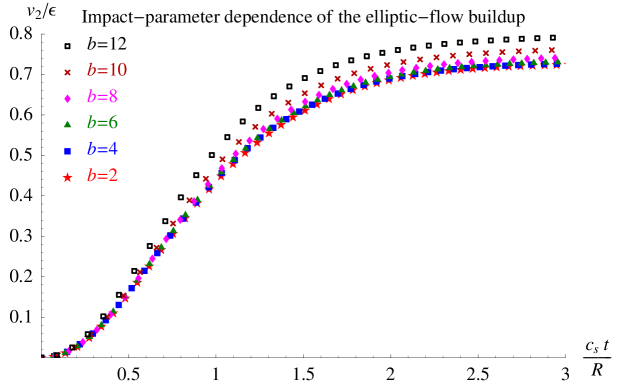
Fig. 1.: Time evolution of $v_{2}/\epsilon$ for different values of the impact parameter, for a gas of massless particles ($c_{s}=1/\sqrt{3}$).

This universal behaviour shows in particular that the typical buildup time for elliptic flow is $\bar{R}/c_{s}$, i.e., about 2–4 fm/$c$ for Au–Au or Cu–Cu collisions, in agreement with the findings of transport-model computations [11, 12].

While Fig. 1 shows that the final $v_{2}$ value depends on the shape of the overlap region, $v_{2}\propto\epsilon$, the scale invariance of ideal fluid dynamics implies that it is independent of the system size, i.e., of $\bar{R}$. Note, however, that this system-size invariance does not allow a straightforward extrapolation from one system to the other (say from Au–Au to Cu–Cu collisions), because the initial conditions do not scale accordingly (different nuclei have different density profiles).

For given system size and shape, the final elliptic-flow value varies with the speed of sound $c_{s}$. More quantitatively, if one assumes a constant $c_{s}$ throughout the system evolution, then the final $v_{2}$ increases with $c_{s}$ as soon as $c_{s}>0.1$ — it even becomes proportional to $c_{s}$ for $c_{s}\gtrsim 0.3$ [7].

To close this Section, let me mention a few results that were obtained analytically, exploiting the fact that the ideal-fluid assumption is equivalent to considering the limit of small freeze-out temperature. In Ref. [13], it was emphasized that emitted particles fall in a natural way into two categories, namely “slow” particles, defined as those whose velocity equals that of the fluid at some point on the freeze-out hypersurface, and “fast” particles, which are faster than the fluid at freeze-out. For both categories of particles, definite predictions regarding anisotropic flow can be made. Thus, the dependence of elliptic flow on the particle velocity $v_{2}(p_{T}/m)$, where $p_{T}$ and $m$ are the particle transverse momentum and mass, should be identical for all types of slow particles (except pions, whose mass is not much larger than the freeze-out temperature). The same property holds for all other flow harmonics $v_{n}(p_{T}/m)$. This in particular implies a mass-ordering of $v_{2}(p_{T})$, the heavier particles having smaller flow at a fixed transverse momentum. It turns out that the mass-ordering of $v_{2}(p_{T})$ also holds for fast particles. For the latter, it was shown that the various even flow harmonics are related, the most important relation being $v_{4}(p_{T})=v_{2}(p_{T})^{2}/2$, valid for each particle species in each rapidity window provided the transverse-velocity profile at freeze-out is not too different from an ellipse [13].

3 Out-of-equilibrium scenario

Let me now turn to the case in which the mean number of collisions per particle, $K{\scriptstyle\!}n^{-1}$, is insufficient to lead to any (local) equilibrium.

3.1 Anisotropic flow in the out-of-equilibrium regime

Determining the precise dependence of anisotropic flow on $K{\scriptstyle\!}n^{-1}$ (as well as on the collision cross sections) requires a transport model which is beyond the scope of the present study, yet general predictions are nonetheless feasible [7].

Thus, it is natural to expect that elliptic flow increase with the number of collisions, since $v_{2}$ vanishes in the absence of final-state interaction, whereas in the large-$K{\scriptstyle\!}n^{-1}$, ideal-fluid limit $v_{2}$ is finite. This growth, however, eventually saturates for some $K{\scriptstyle\!}n^{-1}$ value, for which the system equilibrates (see Fig. 2; ideal-fluid dynamics is expected to yield the maximum $v_{2}$, as hinted at by transport computations, which always give smaller values [14]). The value at which $v_{2}$ saturates obviously depends on the system shape, i.e., on the initial eccentricity $\epsilon$, since $v_{2}\propto\epsilon$ in hydrodynamics; however, the corresponding value of the Knudsen number should be quite independent of $\epsilon$, as individual parton–parton or hadron–hadron interactions do not know anything about the geometry of the nucleus–nucleus collision. As a consequence, the slope in the region where $v_{2}(K{\scriptstyle\!}n^{-1})$ grows should be roughly proportional to $\epsilon$; conversely, the ratio $v_{2}/\epsilon$ should be (almost) independent of the centrality of the collision for a fixed value of $K{\scriptstyle\!}n^{-1}$.

The same reasoning applies to $v_{4}$, which should also increase with the mean number of collisions, and then saturate (at a value $\propto\epsilon^{2}$). If $v_{4}$ does not grow much faster than $v_{2}$, then the ratio $v_{4}/v_{2}^{2}$ is a decreasing function of $K{\scriptstyle\!}n^{-1}$, which reaches a minimum in the ideal-fluid limit. Since the hydrodynamical prediction for the ratio is $1/2$, then $v_{4}>v_{2}^{2}/2$ when equilibrium is not reached [7].

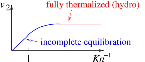
Fig. 2.: Sketchy representation of the variation of $v_{2}$ with the mean number of collisions per particle $K{\scriptstyle\!}n^{-1}$.

In the out-of-equilibrium regime, both $v_{2}$ and $v_{4}$ increase with the number of collisions. Now, $K{\scriptstyle\!}n^{-1}=L/\lambda$ may vary for two reasons, due to changes either in the system size $L$, for which a natural choice is $L=\bar{R}$, or in the mean free path $\lambda$. The former possibility strongly contrasts with the scale invariance of anisotropic flow within the ideal-fluid description [7]. In turn, the mean free path $\lambda=1/n\,\sigma$ depends on both particle density $n$ and cross section $\sigma$, and any change in one of these will affect the Knudsen number, hence the flow coefficients when the system is not equilibrated.

To summarize this part, in an out-of-equilibrium scenario the anisotropic flow coefficients $v_{2}$, $v_{4}$ depend significantly on the system size $\bar{R}$ (even if the system shape $\epsilon$ is fixed), on the particle density and on the interaction cross section, and they are related by $v_{4}/v_{2}^{2}>1/2$, the ratio increasing as one goes further from equilibrium.

3.2 Confronting RHIC data and the out-of-equilibrium scenario

Let me now show that available flow data support the idea that the system created in Au–Au collisions at RHIC is not equilibrated, at least at the time when anisotropic flow develops.

The first element that supports the out-of-equilibrium scenario is its ability to explain the rapidity dependence of elliptic flow [15, 16]. Thus, the fact that $v_{2}(y)$ follows closely the rapidity distribution $dN/dy$ from midrapidity up to the forward regions, where both exhibit the “limiting fragmentation” property across different beam energies [2], is naturally explained within a model where $v_{2}$ varies with the number of collisions per particle. Now, the identity $(c\bar{R}/c_{s})\,n(\bar{R}/c_{s})=(1/S)\,dN/dy$ yields the particle density at the time when anisotropic flow builds up, which gives

$$K{\scriptstyle\!}n^{-1}=\bar{R}\sigma\,n\!\left(\frac{\bar{R}}{c_{s}}\right)=\frac{c_{s}}{c}\frac{\sigma}{S}\frac{dN}{dy},$$ (1)

where $S$ measures the transverse area of the collision zone. Equation (1) shows that the incomplete-equilibration prediction $v_{2}\propto K{\scriptstyle\!}n^{-1}$ translates into $v_{2}(y)\propto dN/dy$. On the other hand, the few 3-dimensional hydrodynamical models cannot reproduce the data, either overestimating $v_{2}(y)$ at intermediate rapidities $y\sim 3$ [15] or, when those values are well predicted, underestimating the midrapidity elliptic flow [17].

A similar instance of experimental result which finds a natural explanation in a non-equilibrium model is the growing discrepancy between $v_{2}(p_{T})$ and the ideal-fluid prediction as transverse momentum increases [18]. As a matter of fact, with increasing $p_{T}$ the interaction cross section is expected to decrease, diminishing the mean number of collisions per particle $K{\scriptstyle\!}n^{-1}\propto\sigma$, which is thus increasingly further from the number needed to ensure equilibration. In turn, this leads to an increase of the difference between the hydrodynamical $v_{2}$ and the out-of-equilibrium value.

One could claim that the previous two arguments concern only a negligible fraction of the particles, while the bulk, at midrapidity and moderately low transverse momenta, would still be in equilibrium. If this were true, then the elliptic flow $v_{2}$ at midrapidity, averaged over transverse momentum, should be proportional to the eccentricity. However, it turns out that the ratio $v_{2}/\epsilon$ is not constant across centralities in Au–Au collisions [3]: the data do not exhibit the scale invariance of ideal fluid dynamics. On the contrary, the values of $v_{2}/\epsilon$ rather seem to be scaling linearly with the control parameter $(1/S)\,dN/dy$ [19], i.e., according to Eq. (1) and assuming that $c_{s}$ and the cross section remain roughly constant for the various centralities, with the number of collisions. This proportionality, without a single hint at any saturation, even extends down to the values measured in Pb–Pb collisions at the CERN SPS, lending further credence to the out-of-equilibrium scenario.

Yet another indication that the system created in Au–Au collisions at RHIC is not equilibrated is provided by the ratio $v_{4}/v_{2}^{2}$. STAR and PHENIX reported values which are significantly larger than the ideal-fluid value of $1/2$ [3, 20].

As a final evidence that approaches based on equilibrium assumptions may not be appropriate at RHIC, let me point out another failure of the ideal-fluid description, which can be resolved provided one drops some equilibrium constraint. Thus, although hydrodynamics describes properly the transverse-momentum dependence of $v_{2}$ of identified particles in minimum bias collisions, on the other hand it misses the centrality dependence of $v_{2}(p_{T})$: the ideal-fluid calculation that reproduce the minimum-bias average overestimate elliptic flow in peripheral events and underestimate its value for pions in central collisions [3]. Even though the former discrepancy is not really surprising — one does not expect the hydrodynamical description to hold for peripheral collisions, where the system size is too small to allow any equilibration —, however the fact that data largely overshoot the so-called ideal-fluid limit in central events is a much more serious issue. A plausible explanation could be that the analysis of the data for these centralities is not fully reliable, which is possible since this is where the anisotropic-flow signal is smallest, hence most difficult to extract accurately. Another possibility is that the central data could indeed be described by ideal fluid dynamics, albeit with a stiffer equation of state, i.e., a larger speed of sound, than what is currently used. This can be done, provided one realizes that the supposedly strong constraint on $c_{s}$ arising from fits to rapidity distributions exists if, and only if, one assumes that the system has reached not only kinetic equilibrium, but also chemical equilibrium. Once this assumption (which is only supported by the success of fits from “thermal” models to particle-abundance ratios, as seen also in $e^{+}e^{-}$ collisions) is dropped, the one-to-one relationship between particle number density, which gives the particle distribution, and energy per particle, which is responsible for flow, disappears, and the constraint on $c_{s}$ is lifted. Allowing now kinetic equilibrium only, one may describe central collisions with a hydrodynamical model — however, even if it proved valid for central events, the ideal-fluid description would not hold in more peripheral collisions.

It could be hoped that a discriminating test between the early-thermalization and out-of-equilibrium scenarios would be provided by measurements of anisotropic flow in Cu–Cu collisions [7]: the change in system size would probe the scale invariance of ideal fluid dynamics, which is broken in the absence of equilibrium. Unfortunately, the preliminary $v_{2}$ results presented at Quark Matter ’05 were quite inconclusive, as the values of the three different experimental Collaborations were not compatible with each other. These discrepancies call for further investigations of the possible sources of systematic error on the measurements, in particular fluctuations of the signal (whether they arise from truly physical effects, or from binning issues) and non-flow effects. The latter were shown to affect the flow analysis in Au–Au collisions, and should be even more important in the smaller Cu–Cu system; several new methods of measurement that are free from their bias were specifically introduced [21, 22] and could be used. Unfortunately, disentangling non-flow effects from fluctuations of the flow itself is not a trivial task [23].

Measurements of anisotropic flow with great accuracy will also be needed to investigate another expected behaviour, namely that the ratio $v_{4}/v_{2}^{2}$ increases at high $p_{T}$ and/or when going away from rapidity, since in both these regimes the measured trends of $v_{2}(p_{T})$ and $v_{2}(y)$ suggest that $K{\scriptstyle\!}n^{-1}$ is decreasing.

Eventually, one can anticipate that anisotropic flow measurements in Pb–Pb collisions at $\sqrt{s_{NN}}=5.5$ TeV at the CERN LHC will help confirm the out-of-equilibrium interpretation of RHIC data. Thus, unless the ideal-fluid limit is marginally reached in the most energetic central Au–Au events at RHIC, the average $v_{2}$ at midrapidity, scaled by the spatial eccentricity, should be larger at LHC than it is at RHIC. Conversely, the ratio $v_{4}(p_{T})/v_{2}(p_{T})^{2}$ should be smaller, approaching the hydrodynamical value of $1/2$.

4 Conclusion

In summary, I have shown that dropping the assumption of kinetic equilibrium at the time when anisotropic flow develops allows me to describe in a satisfactory, consistent manner several features in the flow data that cannot be accommodated in ideal-fluid models. The only instance where a hydrodynamical approach may remain appropriate is in central events; however, even though kinetic equilibrium could be reached, the constraint of chemical equilibrium has to be abandoned if one is to reproduce the $v_{2}$ data.

Although they permit a better description of the data, the predictions of the out-of-equilibrium scenario presented here are admittedly quite crude, and deserve further dedicated studies. A transport model would allow a more quantitative investigation of how the system evolves from an non-equilibrated state to a thermalized one, answering various questions as when (for which value of the Knudsen number) does anisotropic flow reach the hydrodynamical limit? How far are RHIC Au–Au data from this limit? In that respect, the ratio $v_{4}/v_{2}^{2}$ might be a more sensitive indicator than $v_{2}$ itself, as it seems to be further away from the ideal-fluid prediction.

References

- [1] S.S. Adler et al. [PHENIX Collaboration], Phys. Rev. Lett. 91 (2003) 182301.
- [2] B.B. Back et al. [PHOBOS Collaboration], Phys. Rev. Lett. 94 (2005) 122303.
- [3] J. Adams et al. [STAR Collaboration], Phys. Rev. C72 (2005) 014904.
- [4] H. Ito [BRAHMS Collaboration], Proceedings Quark Matter 2005.
- [5] P.F. Kolb and U. Heinz, Quark Gluon Plasma III, eds. R. Hwa & X.-N. Wang, World Scientific, Singapore, 2004, p. 634.
- [6] See the various contributions to these Proceedings.
- [7] R.S. Bhalerao, J.-P. Blaizot, N. Borghini and J.-Y. Ollitrault, Phys. Lett. B627 (2005) 49.
- [8] E.V. Shuryak, Nucl. Phys. A750 (2005) 64.
- [9] N. Borghini, P.M. Dinh and J. Y. Ollitrault, Pramana 60 (2003) 753.
- [10] J.-Y. Ollitrault, Phys. Rev. D46 (1992) 229.
- [11] L. Bravina et al., Phys. Lett. B631 (2005) 109.
- [12] L.-W. Chen and C.M. Ko, preprint nucl-th/0505044.
- [13] N. Borghini and J.-Y. Ollitrault, preprint nucl-th/0506045.
- [14] D. Molnár and P. Huovinen, Phys. Rev. Lett. 94 (2005) 012302.
- [15] T. Hirano, Phys. Rev. C65 (2002) 011901(R).
- [16] U. Heinz and P.F. Kolb, J. Phys. G30 (2004) S1229.
- [17] R. Andrade, F. Grassi et al., preprint nucl-th/0511021.
- [18] D. Teaney, Phys. Rev. C68 (2003) 034913.
- [19] C. Alt et al. [NA49 Collaboration], Phys. Rev. C68 (2003) 034903.
- [20] H. Masui [PHENIX Collaboration], preprint nucl-ex/0510018.
- [21] N. Borghini, P.M. Dinh and J.-Y. Ollitrault, Phys. Rev. C64 (2001) 054901.
- [22] R.S. Bhalerao, N. Borghini and J.-Y. Ollitrault, Nucl. Phys. A727 (2003) 373.
- [23] M. Miller and R. Snellings, preprint nucl-ex/0312008.