A consistent quasiparticle picture of Quark-Gluon plasma and the velocity of sound

Abstract

A thermodynamically consistent density dependent quark mass model has been used to study the velocity of sound in a hot quark-gluon plasma. The results are compared with the recent lattice data.

Key words: Equation of state, Quark Gluon Plasma, Sound velocity To appear in Mod. Phys. Lett. A

The study of the Equation of State (EOS) of strongly interacting matter is of great importance. It can play a vital role for a deeper understanding of many unresolved areas of QCD physics, such as the study of quark-gluon plasma (QGP), quark confinement, phase structure of QCD at high temperature and finite chemical potential, to name a few.

The study of QGP has some formidable problems. Due to the convergence problem in the low energy domain, the widely used perturbative QCD calculation fails badly to give any insight. The most accepted method in this area is the lattice QCD calculation, though the method works better with light dynamical quarks. Moreover, there are difficulties with finite baryon chemical potentials. On the other hand, various phenomenological models of thermodynamical and hydrodynamical types 1 ; 2 ; 3 ; 3a ; 4 ; 5 ; 6 ; 7 ; 7a ; 7b ; 8 ; 9 ; 10 are used as they are easier to handle compared to the lattice. In all these models, a quasiparticle description is used with a background mean field. Here it is worth noting that a quasiparticle description is expected to be applicable, as long as the spectral functions for quarks and gluons resemble qualitatively the asymptotic forms found from HTL (Hard Thermal Loop) perturbative calculations 11 .

The calculations in the quasiparticle description usually start with a Hamiltonian. It was pointed out by Bir$\grave{o}$ et al. 12 that in a Hamiltonian approach, due to the dependence of the Hamiltonian on the thermodynamical characteristics of the surrounding matter, there may be some thermodynamical inconsistency within the method which has to be rectified. To get rid of these inconsistencies, one has to incorporate certain conditions in the quasiparticle model.

In all the studies of the EOS, the sound velocity ($u$), which relates the pressure and the energy as $P=u^{2}E$, plays an important role. Specifically, the QGP is expected to approach the canonical value of $u^{2}=1/3$, at high temperatures and/or densities. An understanding of the quantitative behaviour of the approach to asymptotic freedom is very important, as it is related to the problem of quark confinement.

Another important quantity related to the study of QGP is the quark number susceptibility (QNS), which, being related to charge fluctuation, is of direct experimental relevance. The importance of QNS lies in the fact that it can be used as an independent check on the theoretical models which try to explain the lattice results 13 .

There are numerous results of quark number susceptibility available from lattice calculations 13 ; 14 ; 15 . Also, There have been recent reports of lattice studies where the velocity of sound in a pure gluon plasma at finite temperature has been calculated 16 . Our motivation here is to understand what kind of quasiparticle picture can reproduce these results.

In the present work, we have studied the behaviour of quark number susceptibility and the speed of sound as the quark-gluon plasma moves from the non-perturbative to the perturbative region of QCD. The density dependent quark mass (DDQM) model 17 ; 18 , along with the condition for thermodynamical consistency, has been used for the present study.

The DDQM model aims to explain confinement from a phenomenological point of view. The MIT bag model 1 is so far the simplest option available to explain the confinement phenomenon, though it has some serious shortcomings. The DDQM model is a simple but effective alternate approach to confinement. The main idea behind the DDQM model is to make the mass of the “free” quarks infinitely heavy (confinement) while at small distances, effective quark mass should be small or zero 19 . This behaviour is similar to what is known as “Archimedes Effect” 20 ; 21 .

In the DDQM model, confinement is achieved through a parametrization of the effective quark mass as a function of density. In the low density limit, all the interactions are taken care of by the mass, so that it becomes infinitely large to prevent the occurrence of a single quark in the asymptotic state 17 . The thermodynamical quantities related to the quark sector at finite temperature are calculated from the postulated mass relation and a self-consistent number density relation. At finite temperature the quark mass is defined as 18 ,

$$m(T,n_{q}) = \frac{B}{\Sigma_{i}(n_{i}^{+}+n_{i}^{-})},$$ (1)

where $n_{i}^{+}(n_{i}^{-})$ is the number density of the i-th flavour quark (antiquark) and $n_{q}$ is the net quark number density. These number densities are to be calculated self-consistently from the given relation:

$$n_{i}^{\pm} = \frac{3}{\pi^{2}}\int_{0}^{\infty}dpp^{2}\{\exp[T^{-1}(\epsilon_{i}\mp\mu_{i})]+1\}^{-1},$$ (2)

with,

$$\epsilon_{i}(p,n_{q},T)=[p^{2}+m^{2}(T,n_{q})+\Delta_{i}(p)]^{1/2}$$ (3)

where $\Delta_{i}(p)$ takes care of the divergent term present in the mass at finite temperature. In the zero density limit, $\Delta_{i}(0)=0$ as the mass takes care of all interactions. The expression for $\Delta_{i}(p)$ is given by 18 :

$$d\Delta_{i}(p_{i})\equiv\left\{\frac{6B\pi^{2}c_{i}}{{p_{i}}^{4}}\times\frac{[{p_{i}}^{2}-(B\pi^{2}c_{i}/{p_{i}}^{3})^{2}]}{[{p_{i}}^{2}+(B\pi^{2}c_{i}/{p_{i}}^{3})^{2}]^{1/2}}+\frac{6B^{2}\pi^{4}{c_{i}}^{2}}{{p_{i}}^{7}}\right\}dp_{i}$$ (4)

with $c_{i}\equiv n_{i}/n_{q}$. The energy density and the pressure of the quark system are then readily calculated from

$${\cal E}_{q}=\displaystyle\sum_{i=u,d}\frac{3}{\pi^{2}}\int_{0}^{\infty}dp[p^{2}\epsilon_{i}(p,n_{q},T)(\{\exp[T^{-1}(\epsilon_{i}-\mu_{i})]+1\}^{-1}+\{\exp[T^{-1}(\epsilon_{i}+\mu_{i})]+1\}^{-1})]$$ (5)

$$P_{q}=\frac{1}{3}\displaystyle\sum_{i=u,d}\frac{3}{\pi^{2}}\int_{0}^{\infty}p\frac{\partial\epsilon}{\partial p}{d^{3}}p(\{\exp[T^{-1}(\epsilon_{i}-\mu_{i})]+1\}^{-1}+\{\exp[T^{-1}(\epsilon_{i}+\mu_{i})]+1\}^{-1})$$ (6)

In the gluonic sector, energy density and pressure have the form 18 :

$${\cal E}_{g}=\frac{8}{15}\pi^{2}T^{4}(1-\frac{15\alpha_{c}}{4\pi}),$$ (7)

$$P_{g}=\frac{8}{45}\pi^{2}T^{4}(1-\frac{15\alpha_{c}}{4\pi})$$

Here, $\alpha_{c}$ is the effective gluon-gluon coupling. The form of $\alpha_{c}$ is given by 18 :

$$\alpha_{c}=\frac{54B\pi^{3}}{(<Q^{2}>_{n_{q},T})^{2}}$$ (8)

where,

$$<Q^{2}>_{n_{q},T}=\frac{4}{3}\frac{\displaystyle\sum_{i}(n_{i}^{+}+n_{i}^{-})<Q^{2}>_{i}+n_{g}<Q^{2}>_{g}}{\displaystyle\sum_{i}(n_{i}^{+}+n_{i}^{-})+n_{g}}$$ (9)

$<Q^{2}>_{i}$ and $<Q^{2}>_{g}$ are the thermal average of the three momentum squared of quarks of flavour i and gluons. $<Q^{2}>_{g}$ corresponds to non-interacting gas of gluons, $n_{g}$ being the gluon number density 18 ; 22 .

So the total energy density and pressure of the quark-gluon plasma is,

$${\cal E}_{QGP}={\cal E}_{q}+{\cal E}_{g},P_{QGP}=P_{q}+P_{g},$$ (10)

In the regions of low temperature and density, the energy density and pressure of the gluonic sector becomes negative which can be interpreted as the signal of the formation of gluonic condensates. As long as the gluons remain in the condensed phase they do not contribute explicitly to the thermodynamic quantities (they are not active degrees of freedom of the system). So, ${\cal E}_{g}$ = ${\cal P}_{g}$ =0 for $\alpha_{c}\geq\frac{4\pi}{15}$ 18 .

The DDQM model has been widely used in the literature for the study of dense quark matter 23 ; 24 ; 25 ; 26 ; 27 ; 28 , the thermodynamical inconsistency notwithstanding 12 . Let us now modify the above EOS incorporating the conditions of thermodynamical consistency. The prescription for ensuring thermodynamical consistency is to introduce a ”background” field $\Phi$ which should satisfy the following conditions 12 ;

$$\frac{\partial\Phi}{\partial T}+\displaystyle\sum_{j=u,d}d_{j}\int\frac{d^{3}k}{(2\pi)^{3}}\frac{\partial\epsilon_{kj}}{\partial T}\nu_{kj} = 0,$$ (11)

$$\frac{\partial\Phi}{\partial n_{i}}+\displaystyle\sum_{j=u,d}d_{j}\int\frac{d^{3}k}{(2\pi)^{3}}\frac{\partial\epsilon_{kj}}{\partial n_{i}}\nu_{kj} = 0.$$ (12)

where $d_{j}$ is the degeneracy factor and $\nu_{kj}$ is the average quasiparticle occupation number of j-th flavour quark with momentum k:

$$\nu_{kj}=(\{\exp[T^{-1}(\epsilon_{j}-\mu_{j})]+1\}^{-1}+\{\exp[T^{-1}(\epsilon_{j}+\mu_{j})]+1\}^{-1})]$$ (13)

In the present case, the above two conditions become,

$$\frac{\partial\Phi}{\partial T}+\displaystyle\sum_{j=u,d}n^{(s)}_{j}\frac{\partial m_{j}}{\partial T} = 0,$$ (14)

$$\frac{\partial\Phi}{\partial n_{i}}+\displaystyle\sum_{j=u,d}n^{(s)}_{j}\frac{\partial m_{j}}{\partial n_{i}} = 0.$$ (15)

where $n^{(s)}_{j}$ is the scalar quasiparticle density of j-th flavour quark,

$$n^{(s)}_{j} = d_{j}\int\frac{d^{3}k}{(2\pi)^{3}}\nu_{kj}\frac{m_{j}}{\epsilon_{j}}$$ (16)

In the present paper we have considered a two flavour QGP system. Since $u$ and and $d$ quarks have equal masses, our system, in essence, consists of one type of quasiparticles only (except for the degeneracy factor 2 for two flavours). So, the quasiparticle quark mass depends on temperature and quasiparticle density through the scalar density only and the expression for the background field $\Phi$ reduces to

$$\Phi=-\int\displaystyle\sum_{j=u,d}n^{(s)}_{j}dn_{j}$$ (17)

Carrying out the integration and identifying the integration constant with $\Phi=0$ at T=0, $n_{B}=0$, background field $\Phi$ can be obtained. At zero temperature, $\Phi$, naturally, depends on the baryon density ($n_{B}$) alone. With this background field, we define thermodynamically consistent energy density and pressure as,

$${\cal E}_{QGP}={\cal E}_{q}+{\cal E}_{g}+\Phi(n_{B},T)$$ (18)

$$P_{QGP}=P_{q}+P_{g}-\Phi(n_{B},T)$$ (19)

At zero temperature and density, the total energy density of the QGP becomes B, the energy of an empty bag. On the other hand, the pressure of QGP becomes zero and we do not encounter the unphysical negative pressure as found in most of the MIT bag like phenomenological models. It is to be noted here that there is no bag pressure in this model as such. Since the mass of the quark becomes infinitely large in the density going to zero limit, a negative bag pressure would amount to double counting 17 .

We define the baryon ($n_{i=0}$) and isospin ($n_{i=3}$) densities and the corresponding susceptibilities as:

$$n_{i}=\frac{T}{V}\frac{\partial ln\cal{Z}}{\partial\mu_{i}},\ \ \chi_{ij}=\frac{T}{V}\frac{\partial^{2}ln\cal{Z}}{\partial\mu_{i}\partial\mu_{j}}.$$ (20)

where, $\cal{Z}$ is the partition function and thermodynamic potential $\Omega$ is defined as $\Omega=-P_{QGP}=-Tln\cal{Z}$. Also $\mu_{i=0}=\mu_{u}+\mu_{d}$ and $\mu_{i=3}=\mu_{u}-\mu_{d}$.

In figure 1 and 2 we have plotted $\chi_{3}/\chi_{FFT}$ as a function of $T/T_{c}$. Here $\chi_{3}$ is the iso-vector susceptibility and $\chi_{FFT}$ is the free field value; for details see 29 ; 30 . It is to be noted here that the value of the critical temperature in figure 1 and 2 are different. In figure 1 the $T_{c}$ is taken from the consideration of the commonly held belief that the QCD critical temperature is between 150-200 MeV; in our calculation it is taken to be 200 MeV and represented by dash-dot curve. In figure 2 the critical temperature has been calculated from the DDQM (taking the zero pressure limit, beyond which quark matter system will become unstable) and shown as continuous line in the graph. The points are from lattice calculation 13 for different values of the valence quark mass. As seen from the plot, our result is in qualitative agreement with the lattice result in the region near the critical temperature. But at higher temperature it approaches the ideal gas limit faster than what we get from the lattice calculation. Here it is worth mentioning that in our calculation current quark mass is zero and the dynamic quark mass varies with temperature.

The variation of $\Phi$ with temperature at three different baryon densities for B^1/4=145 MeV is shown in figure 3. The value of $\Phi$ is maximum for $n_{B}=0$ and it decreases for increasing density. This behaviour of of $\Phi$ could have been anticipated, as the system is expected to be closer to the perturbative domain at higher densities. Near the transition temperature $T_{c}$, $\Phi$ shows a rapid variation and then saturates at high temperature. In fact, around the saturation region the effect of $\Phi$ on thermodynamic quantities becomes negligibly small. In figure 4, we have plotted ($\cal{E}$-3p)/T⁴ with temperature. The two curves are for the cases with and without the background field $\Phi$; B^1/4 and $n_{B}$ being fixed at 145 MeV and 3n₀ (where n₀ = 0.17 $fm^{-3}$ is the nuclear matter saturation density) respectively. The continuous and the broken lines correspond to the cases with and without the background field contribution, respectively. Inclusion of the background field into the model increases the critical temperature by $29\%$ in the DDQM. The non-perturbative effects are dominant near the transition temperature. The inclusion of thermodynamic consistency certainly enhances these effects, as seen in figure 4. Similar behaviour is obtained for the other values of B as well.

Our main motivation in this paper has been to study the velocity of sound, which is given by $(\frac{\partial P}{\partial{\cal E}})_{S}$. But in the present paper we have plotted $(\frac{\partial P}{\partial{\cal E}})_{T}$, as it is easier to compute in the present model. Moreover, it was pointed out in ref.18 that the difference between $(\frac{\partial P}{\partial{\cal E}})_{T}$ and $(\frac{\partial P}{\partial{\cal E}})_{S}$ does not exceed 10%. The figures 5, 6, 7 and 8 show the variation $(\frac{\partial P}{\partial{\cal E}})_{T}$ as a function of temperature for different densities at B^1/4=145 MeV. We have also presented the recent results from lattice calculation 16 . As mentioned earlier, the dash-dot curves in figures 6 and 8 are plotted with $T_{c}$ equal to 200 MeV. The continuous and the broken lines in figures 5 and 7 correspond to the cases with and without the background field contribution, respectively, the $T_{c}$ being calculated from the DDQM.

As seen from all the plots, $(\frac{\partial P}{\partial{\cal E}})_{T}$ is greatly modified by the contribution from the background field around $T_{c}$; $\Phi$ has a dominant effect near $T_{c}$. Moreover, as $\Phi$ goes over to B at zero temperature and density, the change in B affects the sound velocity much more than that due to the change in density. It is to be noted here that the lattice results for sound velocity 16 presented here are for gluonic contribution only, whereas our results are for quark gluon plasma. The discontinuity in the plot is due to the built-in second order phase transition (gluon condensate) in the present EOS.

Here we would like to point out that in figures 7 and 8, we have compared our results for the speed of sound in QGP at non-zero $n_{B}$ with the lattice values at $n_{B}=0$. These comparisons indicate that the behaviour near $T_{c}$ is governed mainly by the physics of confinement. In our model, the presence of quarks (along with the gluons) has very small effect on the in-medium behaviour of sound velocity.

To conclude, we have studied the velocity of sound in the QGP with a thermodynamically consistent DDQM model. This is a one parameter model and the dependence on the parameter is also seen to be very weak. This is the remarkable feature of this model. Incorporation of thermodynamic consistency produces qualitatively and semi-quantitatively, the features of the lattice data and also explains all the necessary features of the non-perturbative to perturbative transition of the QCD physics. Our study shows that the incorporation of consistency condition is essential to understand the nonperturbative behaviour near transition temperature. The result obtained for QNS falls within the range of lattice data. The result for the sound velocity of quark gluon plasma for zero baryonic density at critical temperature 200 MeV is in qualitative agreement with the lattice result for pure gluon plasma. Our result of sound-velocity of QGP for the finite baryonic density may be considered as a prediction to be confirmed by the future lattice calculations.

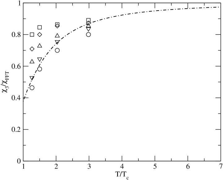
Figure 1: Variation of $\chi_{3}/\chi_{FFT}$ with temperature for B^1/4=145 MeV ,n_B=0 and $T_{c}=200MeV$. Dash-dot curve represents our model calculation. Different symbols like circle, down-triangle, up-triangle,diamond and the square represent lattice data corresponding to the valence quark mass 1.0, 0.75, 0.5, 0.3, 0.1, in units of $T_{c}$, respectively 13 .

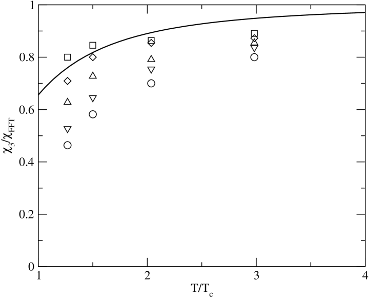
Figure 2: Variation of $\chi_{3}/\chi_{FFT}$ with temperature for B^1/4=145 MeV ,n_B=0 and T_c=330 MeV, calculated from the model. Solid curve represents our model calculation. Different symbols like circle, down-triangle, up-triangle, diamond and the square represent lattice data corresponding to the valence quark mass 1.0, 0.75, 0.5, 0.3, 0.1, in units of $T_{c}$, respectively 13 .

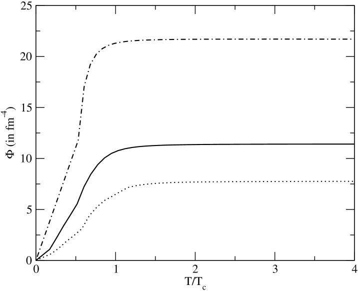
Figure 3: Variation of $\Phi$ with temperature for B^1/4=145 MeV. Dash-dot, solid and dotted curves are for densities n_B=0, n_B=3n₀ and n_B=4n₀ respectively, $n_{0}$ being the nuclear matter saturation density. Critical temperature for n_B=0 is 330 MeV, for n_B=3n₀ it is 290 MeV and for n${}_{B}=4n_{0}$ it is 260 MeV.

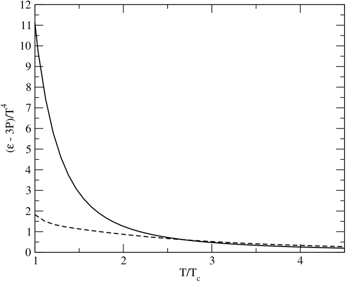
Figure 4: Variation of ($\cal{E}$-3P)/T⁴ with temperature for B^1/4=145 MeV, n_B=3n₀ and $T_{c}=290MeV$. Solid and dash curves correspond to the cases with and without $\Phi$ contributions, respectively.

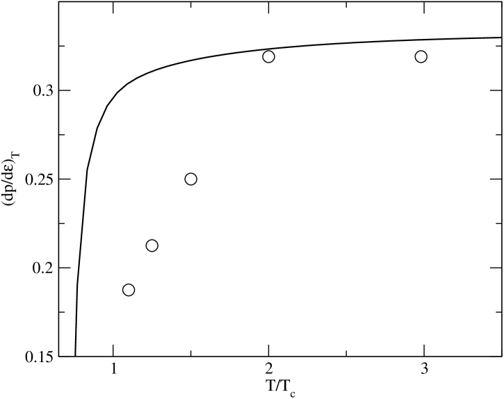
Figure 5: Variation of $(\frac{\partial P}{\partial{\cal E}})_{T}$ with temperature for B^1/4=145 MeV, n_B=0 and $T_{c}=330MeV$ calculated from the model. Lattice data (circles) are taken from 16 . Solid line is for our model.

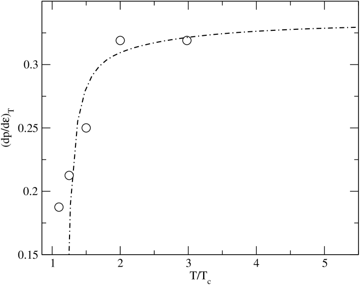
Figure 6: Variation of $(\frac{\partial P}{\partial{\cal E}})_{T}$ with temperature for B^1/4=145 MeV, n_B=0 and $T_{c}=200MeV$. Lattice data (circles) are taken from 16 . Dash-dot line is for our model.

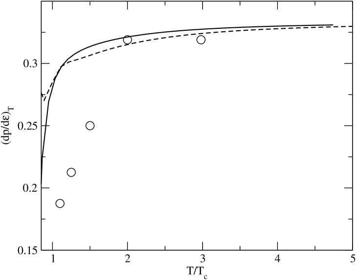
Figure 7: Variation of $(\frac{\partial P}{\partial{\cal E}})_{T}$ with temperature for B^1/4=145 MeV, n_B=3n₀ and $T_{c}=290MeV$, calculated from the model. Lattice data (circles) are taken from 16 . Solid and the broken lines correspond to the cases with and without $\phi$ contributions, respectively.

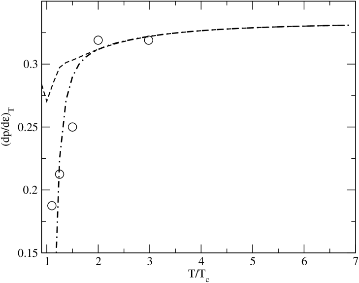
Figure 8: Variation of $(\frac{\partial P}{\partial{\cal E}})_{T}$ with temperature for B^1/4=145 MeV, n_B=3n₀ and $T_{c}=200MeV$. Lattice data (circles) are taken from 16 . Dash-dot and the broken lines correspond to the cases with and without $\phi$ contributions, respectively.

References

- (1) A.Chodes, R.L.Jaffe, K.Johnson, C.B.Thorn, Phys.Rev.D10, 2599 (1974).
- (2) R.Giles, Phys.Rev.D13, 1670 (1976).
- (3) G.A.Miller, A.W.Thomas, S.Theberge, Phys.Lett.B91, 192 (1980).
- (4) S.Lee, K.J.Kong, Phys.Lett.B 202, 21 (1988).
- (5) J.Alam, B.Sinha, S.Raha, Phys.Rept.273, 243 (1996).
- (6) P.Levai, U.Heinz, Phys.Rev.C57, 1879 (1998).
- (7) A.Peshier, B.Kmpfer, G.Soff, Phys.Rev.C61, 045203 (2000).
- (8) J.Cleymans, M.I.Gorenstein, J.Stalnacke, E.Suhonen, Phys.Scr. 48, 277 (1993).
- (9) V.K.Tiwari, N.Prasad, C.P.Singh, Phys.Rev.C58, 439 (1998).
- (10) A.Kostyuk, M.I.Gorenstein, S.Stoecker, W.Greiner, Phys.Rev.C63, 044901 (2001).
- (11) E.Nikonov, A.Shanenko, V.Toneev, Heavy Ion Physics 8, 89 (1998).
- (12) H.W.Barz, B.L.Friman, J.Knoll, H.Schulz, Nucl.Phys.A484, 661 (1988).
- (13) T.S.Bir, P.Levai, J.Zimnyi, J.Phys.G25, 1311 (1999).
- (14) M.A.Thaler, R.A.Schneider, W.Weise, Phys.Rev.C 69, 035210 (2004).
- (15) T.S.Bir, A.A.Shanenko, V.D. Toneev, Phys.Atom.Nucl. 66, 982 (2003).
- (16) R.V.Gavai, S.Gupta, hep-ph/0502198.
- (17) S.Gottlieb, W.Liu, D.Toussaint, R.L.Renken and R.L.Sugar, Phys.Rev.Lett 59, 2247 (1987).
- (18) P.Chakraborty, M.G.Mustafa and M.H.Thoma, Phys. Rev. D68, 085012 (2003).
- (19) R.V.Gavai, S.Gupta, S.Mukherjee hep-lat/0506015.
- (20) G.N.Fowler, S.Raha, R.M.Weiner, Z.Phys.C 9, 271 (1981).
- (21) M.Plmer, S.Raha, R.M.Weiner, Phys. Lett.139B, 198 (1984).
- (22) S.Eliezer, R.Weiner, Phys. Rev.D13, 87 (1976).
- (23) J.C.Pati, A. Salam, Proceedings of the International Neutrino Conference. Aachen, West Germany, 1976.
- (24) D.A.Dicus, J.C.Pati, V.L.Teplitz, Phys. Rev D21, 922 (1980).
- (25) J.I.Kapusta, Nucl. Phys. B148, 461 (1979).
- (26) Y.Zhang, R.K.Su, J.Phys.G30, 811 (2004).
- (27) Y.Zhang, R.K.Su, Phys.Rev.C65, 035202 (2002).
- (28) P.Wang, Phys.Rev.C62, 015204 (2000).
- (29) G.X.Peng, H.C.Chiang, J.J.Yang, L.Li, B.Liu, Phys.Rev.C61, 015201(2000).
- (30) G.Lugones, O.G.Benvenuto, Phys.Rev.D52, 1276 (1995).
- (31) O.G.Benvenuto, G.Lugones, Phys.Rev.D51, 1989 (1995).
- (32) R.V.Gavai, S.Gupta, Phys.Rev.D65, 094515 (2002).
- (33) R.V.Gavai, S.Gupta, hep-ph/0507023.