Shape mixing in the $A\approx 70$ region

Abstract

We investigate the mixing of different shapes in the $A\approx 70$ region using the adiabatic self-consistent collective method in a rotating nuclei. The calculation is done for ⁶⁸Se and ^72-78Kr which are known to show oblate-prolate shape coexistence at low angular momentum. A pairing-plus-quadrupole Hamiltonian, which is known to reproduce reproduce the structure nuclei in this mass region, is used. We calculate the collective path between the oblate and prolate minima and discuss how the collective behaviour of the system changes with increasing angular momentum.

I Introduction

The question “what is the shape” of a nucleus is an old one, and probably dates back to the introduction of Bohr’s liquid drop model BK37 . Modern nuclear physics has tried to find answers to this question in many areas of the table of isotopes. One area of extreme experimental interest is the $N\approx Z$ region for intermediate mass, where all the simple models tell us nuclear dynamics rapidly changes with proton and neutron number. Such proton-rich nuclei are also important in the RP-process of nucleo-synthesis, and are of interest since they are only accessible with modern experimental facilities.

Mean-field methods are one way to give microscopic meaning to the concept of nuclear shape. They have been used quite extensively in nuclear physics RS80 , since they give a good starting point for the description of many but the lightest of nuclei. There are a large number of improvements one can make, either at a single minimum in the mean-field energy (random phase phase approximation, projection techniques, quasi-particle expansions), or in the case that a single minimum is insufficient (time-dependent Hartree-Fock and related methods, Hill-Wheeler method, etc.).

In this work we shall apply the theory of large-amplitude collective motion DK00 , which is a method that tries to describe, in a self-consistent fashion, a few-dimensional surface in which most of the low-energy dynamics takes place. There are many related methods in use in many areas of physics, see e.g. To98 . Our method is just one of a large set of techniques applied to this problem in nuclear physics DK00 .

Even though it is derived in a very different way, it shows great similarity to the Hill-Wheeler method, which relies on the constrained Hartree-Fock Bogoliubov (CHFB) technique. Here a set of Slater determinants determined by a small set of judiciously chosen one-body constraints is used to map out what is presumably a dominant part of the space of all configurations. The analogy with the technique of generating states for specified angular momentum by imposing constraints (cranking) leads to the name “generalised cranking”. The one-body constraints usually consist of a few carefully chosen multipole, or particle-hole, operators, as well as a few generalised pairing, or particle-particle, ones. For large scale realistic problems such as the description of nuclear fission the number of generalised cranking operators needed in order to make a realistic calculation can become very large. There is also no reason to limit the constraints to the standard choices; other degrees of freedom, especially those involving spin-orbit interactions might also be important. A more satisfactory method should allow the cranking operators to be determined by the nuclear collective dynamics itself.

One such approach, followed in this paper and set out in detail in the review paper Ref. DK00 as well as in Ref. AW04 (a similar approach, plus relevant references, can be found in Refs. MN00 ; KN03 ; KN04 ; KN05 ), leads to a very well-defined approach, which can in principle be solved knowing the Hamiltonian and model space. To find the adiabatic collective path we use the local harmonic approximation (LHA). It consists of a constrained mean-field problem that needs to be solved together with a local random phase approximation (RPA), which determines the constraining operator. This approach lacks practicality, since the size of the RPA problem is, for a system with pairing, proportional to the size of the single-particle space squared. Even though enormous matrices can routinely be diagonalised on modern computer systems, the algorithm requires repeated diagonalisation of such a matrix, which makes an implementation in realistic calculations prohibitively time consuming. A practical solution to this problem was given in Ref. NW99 ; AW03 ; AW04 . It consist of solving the RPA in a limited basis of state dependent operators. This was shown to give excellent results for low lying RPA solutions in the minimum as well as along the collective path. Our Japanese colleagues have developed an interesting alternative based on the full RPA for separable forces, which can be solved by dispersion relations KN03 ; KN04 ; KN05 .

In this paper we set out to study the the collective motion in rotating nuclei. The method is a generalised version of the method presented in Ref. AW04 where we study collective path at a given angular momentum AW04b . Experimental results show a large variety of shape-coexistence phenomena at low angular momentum in the mass-region around ⁷²Kr FB00 ; BM03 ; CR97 ; BK99 ; KC05 . This is therefore a good testing ground for large amplitude collective motion calculations in rotating nuclei.

II Formalism

Details of the formalism can be found in our previous work, specifically Refs. DK00 ; AW04 . It is based on time-dependent mean field theory, and the fact that this is a form of classical Hamiltonian dynamics. The issue of selecting collective coordinates can then be separated in two steps, the determination of the Hamiltonian governing the classical mechanics and the approximate decoupling of a few modes in classical mechanics. To facilitate the second task, we usually make the additional assumption of slow motion, called the adiabatic approximation. In that limit, it sufficed to expand the Hamiltonian to second order in momenta, and we have a problem that can be solved in closed form. The solution, as succinctly summarised below, can be stated without any reference to the original nuclear many-body problem and the choice of the interaction. The alternative method set out in Ref. MN00 looks rather different, and relies heavily on the use of Slater determinants. As discussed in the appendix, it is very close to our work and only differs in small details .

II.1 Local harmonic approximation for the collective path in the adiabatic limit

By parameterising the expectation value of the quantum-Hamiltonian with a set of classical coordinates, which corresponds to a classical boson mapping of the density matrix DK00 , we can parametrise the Hamiltonian locally in terms of a set of coordinates and momenta. Clearly, we could also work in the language of differential forms, and avoid specifying coordinates, and coordinate frames that are chosen differently at different points AM88 . Such elegance would hide the technical aspects of obtaining a suitable algorithm.

We assume a classical Hamiltonian depending on a set of real canonical coordinates, $\xi^{\alpha}$ ($\alpha=1,\ldots,N$), and conjugate momenta, $\pi_{\beta}$ ($\beta=1,\ldots,N$). The potential $V(\xi)={\cal H}(\pi=0)$ and the mass matrix $B^{\alpha\beta}$ are given by an expansion of ${\cal H}(\xi,\pi)$ in powers of $\pi$ in zeroth and second order, respectively,

$${\cal H}(\xi,\pi)=V(\xi)+\frac{1}{2}B^{\alpha\beta}\pi_{\alpha}\pi_{\beta}+{\cal O}(\pi^{4}).$$ (1)

Terms of higher order (such as $\pi^{4}$) are supposed to be negligible. The central part in our approach to large amplitude motion is a search for collective (and non-collective) coordinates $q^{\mu}$ which are obtained by an invertible point transformation of the original coordinates $\xi^{\alpha}$, preserving the quadratic truncation of the momentum dependence of the Hamiltonian, by

$$q^{\mu}=f^{\mu}(\xi),\quad\xi^{\alpha}=g^{\alpha}(q)\quad\left(\mu,\alpha=1,\ldots,n\right),$$ (2)

and the corresponding transformation relations for the momenta $p_{\mu}$ and $\pi_{\alpha}$,

$$p_{\mu}=g^{\alpha}_{,\mu}\pi_{\alpha},\quad\pi_{\alpha}=f^{\mu}_{,\alpha}p_{\mu}\quad,$$ (3)

where we use a standard notation for the derivatives, $g^{\alpha}_{,\mu}\equiv\frac{\partial}{\partial q^{\mu}}g^{\alpha}$ and $f^{\mu}_{,\alpha}\equiv\frac{\partial}{\partial\xi^{\alpha}}f^{\mu}$. The adiabatic Hamiltonian, Eq. (1), is then transformed into

$$\bar{{\cal H}}(q,p)=\bar{V}(q)+\frac{1}{2}\bar{B}^{\mu\nu}p_{\mu}p_{\nu}+{\cal O}(p^{4})$$ (4)

in the new coordinates. The new coordinates $q^{\mu}$ are to be divided into three categories: the collective coordinate $q^{1}$, the zero-mode coordinates $q^{I}$, $I=2,\ldots,M+1$, which describe motions that do not change the energy and finally the non-collective coordinates $q^{a}$, $a=M+2,\ldots,n$.

The collective coordinate is determined by means of the solution to the local harmonic approach, which consists of a set of self-consistent equations. These are:

1. The force equations

   $$\bar{{\cal H}}_{,\alpha}=\Lambda f_{,\alpha}+\Lambda_{I}f^{I}_{,\alpha},$$ (5)

   where $f^{I}$ are the zero-modes (also called Nambu-Goldstone or spurious modes) and $\Lambda_{I}$ represents a set of Lagrange multipliers (which in nuclear physics are sometimes called cranking parameters). $\Lambda$ is a Lagrange multiplier for the collective mode, stabilising the system away from equilibrium (we shall often call it the generalised cranking parameter).

2. The local RPA equation

   $$\bar{V}_{;\alpha\gamma}B^{\gamma\beta}f_{,\beta}=\left(\hbar\Omega\right)^{2}f_{,\alpha},$$ (6)

   where the covariant derivative $V_{;\alpha\beta}$ is defined in the usual way ($V_{,\alpha\beta}=(V_{,\alpha})_{,\beta}$). Zero modes correspond to zero eigenvalues of the RPA. In principle great care needs to be taken to have zero modes behave correctly away from equilibrium. The symplectic RPA DK00 is the correct way to do so; unfortunately it is rather cumbersome. Below we will discuss an alternative approach to remove the admixture of spurious solution in an approximate scheme.

The collective path is found by solving Eqs. (5) and (6) self-consistently, i.e., we look for a path consisting of a series of points where the lowest non-spurious eigenvector of the local RPA equations also fulfils the force condition. The motion along this line does not necessarily decouple from other degrees of freedom, but we have a “decoupling measure” $D$, that measures how good or bad this coupling is. As discussed in Ref. DK00 , it measures the change of non-collective coordinates for a change in the collective one, which must be zero for exact decoupling. In the minimum of the potential the spurious solutions decouple from the other collective and non-collective solutions, and spurious admixtures are absent. This is not true for other points along the collective path, especially when approximations are made Yo04 , see the further discussion in Sec. II.3.

II.2 Pairing+quadrupole model

We apply the LHA to the pairing+quadrupole Hamiltonian as described in BK68 . With a constraint on both angular momentum and particle numbers the Hamiltonian can be written as

$$H^{\prime} = H-\sum_{\tau=n,p}\mu_{\tau}N_{\tau}-\omega J,$$ (7)

$$H = \sum_{l}\epsilon_{l}c^{\dagger}_{k}c_{k}-\sum_{\tau=n,p}\frac{G_{\tau}}{2}\left(P^{\dagger}_{\tau}P_{\tau}+P_{\tau}P^{\dagger}_{\tau}\right)-\frac{\kappa}{2}\sum_{M=-2}^{2}Q^{\dagger}_{2M}Q_{2M},$$ (8)

where $\epsilon_{l}$ are spherical single-particle energies, $N_{\tau}$ are the particle number operators, $J$ is the angular momentum operator, $Q_{2M}$ is the dimensionless quadrupole operator

$$Q_{2M}=\frac{1}{\sqrt{2}b^{2}_{0}}\sum_{kl}\left<k\right|r^{2}Y_{2M}\left|l\right>c^{\dagger}_{k}c_{l},$$ (9)

where $b_{0}=1/\sqrt{\omega_{0}}$ is the standard oscillator length and $P^{\dagger}_{\tau}$ is the (dimensionless) pairing operator

$$P^{\dagger}_{\tau}=\sum_{k>0}c^{\dagger}_{k}c^{\dagger}_{-k}\quad.$$ (10)

In Eqs. (7–10) $c^{\dagger}_{k}$ ($c_{k}$) are the single particle creation (destruction) operators, where $k$ labels a set of quantum numbers. The Hamiltonian (7) is treated in the Hartree-Bogoliubov approximation and it has been shown that at the minimum the local RPA for this Hamiltonian is equivalent to the quasi-particle RPA.

The spherical single-particle energies are calculated from a modified spherical oscillator NR95 . The interaction strengths (see Table 1) are chosen to give realistic values of the deformation and pairing gaps in the ground states.

Table 1: The interaction strengths used in the calculations.

	$\kappa$ [MeV]	$G_{n}$ [MeV]	$G_{p}$ [MeV]
68Se	0.09894	0.3437	0.3441
72Kr	0.091	0.3469	0.3514
74Kr	0.08643	0.3333	0.3357
76Kr	0.08473	0.3204	0.3326
78Kr	0.08452	0.3077	0.3287

Our model space consists of two major shells. We follow BK68 and multiply each quadrupole matrix element with a $N$-dependent scaling factor. To achieve the same root-mean-square radii for protons and neutrons different harmonic oscillator frequencies are adopted for each type of nucleons BK68 . The deformation parameters $\epsilon_{2}$ and $\gamma$ are calculated from the expectation values of the $Q_{0}$ and $Q_{2}$ operators as

$$\epsilon_{2} = \frac{3}{2}\frac{\kappa}{\hbar\omega_{0}}\sqrt{\left<Q_{0}\right>^{2}+\left<Q_{2}\right>^{2}},$$ (11)

$$\gamma = \tan^{-1}\left(\frac{\left<Q_{2}\right>}{\left<Q_{0}\right>}\right).$$ (12)

II.3 Removing spurious admixtures in RPA

Two of the main difficulties of applying the LHA method to realistic nuclear problems are the effort required in diagonalising the large-dimensional RPA matrix repeatedly within the double iterative process and the problem of spurious admixtures into the collective path. To limit the computational effort we use the method presented in Ref. NW99 ; AW04 to reduce the size of the RPA matrix. There it was shown that the RPA equation can be solved with good accuracy by assuming that the RPA eigenvectors can be described as a linear combination of a small number of state-dependent one-body operators. The same set of operators turned our to give good bases for solving the RPA problem also at finite angular momentum AW04b . To avoid problem with spurious admixture in our collective coordinate me remove the spurious admixture from our state dependent basis set.

We select a small number of state dependent one-body operators $F^{(k)}$, $k=1,\ldots,n$, assuming that the RPA eigenvectors can be approximated as linear combinations of the $F^{(k)}$. The approximate RPA vector $\bar{f}_{,\alpha}$ is then given by

$$f_{,\alpha}\approx\bar{f}_{,\alpha}=\sum_{k=1}^{n}b_{k}{\cal F}^{(k)}_{,\alpha}$$ (13)

where ${\cal F}^{(k)}$ is the expectation value of $F^{(k)}$. Any spurious admixture to this basis RPA vector is removed by enforcing that the vector ${\cal F}^{(k)}$ is perpendicular to the spurious particle number and angular momentum operators. This new basis set $\tilde{\cal F}^{(k)}$ is given by

$$\tilde{{\cal F}}^{(k)}={\cal F}^{(k)}-\sum_{i}d_{i}^{k}O^{(i)}\quad,$$ (14)

where $O^{(i)}$ are the particle number and angular momentum operators. The coefficients $d_{i}^{k}$ can be found by enforcing the condition

$$\tilde{{\cal F}}^{(k)}\cdot O^{(j)}=0\quad,$$ (15)

which leads to a system of linear equations which can be solved for $d_{i}^{k}$. Even though the removal of the spurious admixture is of principal importance it turns out to only give a small change to the collective path for the example of ⁷²Kr as studied in Ref. AW04b .

II.4 Schrödinger equation on the collective path

After having made a semi-classical approximation, which leads to a classical Hamiltonian, we need to remember that we are studying a quantum system. The standard technique to deal with this is to treat the classical Hamiltonian as a quantum one, and to calculate the eigenfunctions and energies. One must include the zero modes when quantising the Hamiltonian, since they describe rotational and other excitations. Quantisation of the Hamiltonian in a metric coordinate space turns the kinetic energy into a Laplace-Beltrami operator (see, e.g., Ref. AM88 ) in the relevant space and the collective Schrödinger equation can then be written as

$$H(\boldsymbol{X})\Psi(\boldsymbol{X})=E\Psi(\boldsymbol{X})$$ (16)

where $\boldsymbol{X}$ represent both the collective coordinate Q and the spurious coordinates.

Since the potential and the masses are independent of the zero-mode coordinates the wave-function $\Psi$ can be separated into various pieces,

$$\Psi(Q,\phi_{N},\phi_{P},\Omega)=g^{-1/4}U(Q)\frac{1}{\sqrt{2\pi}}e^{im\phi_{N}}\frac{1}{\sqrt{2\pi}}e^{ik\phi_{P}}D^{I}_{MK}(\Omega)^{*}$$ (17)

where $m$ and $k$ are the quantum numbers for neutron and proton pairing rotation, and $I,M,K$ are the usual rotator quantum numbers. We shall be looking at ground states (band-heads) only, and therefore we shall now use $I=M=K=0$, and since pairing rotational excitation corresponds to a change in particle number, we shall be use $m=k=0$ as well. Using (17) to separate variables, the Schrödinger equation (16) can be written as

$$-g^{-1/4}\frac{\partial}{\partial Q}\left(g^{1/2}\frac{\partial}{\partial Q}g^{-1/4}U(Q)\right)+V(Q)U(Q)=EU(Q).$$ (18)

Since we wish the wave function $\Psi$ to be normalisable we require it to be finite, and we must then insist that $U(Q)$ goes to zero when $g$ does. In the present work that only occurs when either of the pairing gaps collapses and thus $B_{\phi_{P,N}}=0$ is zero, and we shall ignore the rotational moments of inertia, which do not change very quickly. Below we solve Eq. (18) on a grid with the boundary condition that $U(Q_{\rm max})=U(Q_{\rm min})=0$. At points where $B_{\phi}=0$ the condition $U=0$ holds exactly; for other cases applying this boundary condition will only give an upper limit on energy.

III Results

We have performed calculations for a chain of Krypton isotopes in the $A=70$ region, to study the effect of changing neutron number on the behaviour of these nuclei. To compare with previous work KN04 ; KN05 , we have also studied the nucleus ⁶⁸Se, which will be seen below to be behave in a rather similar way as some of the Krypton nuclei.

III.1 ⁶⁸Se

The nucleus ⁶⁸Se is of key interest since it has equal numbers of protons and neutrons. It has also been investigated using similar methods for $J=0^{+}$ by Matsuo et al. KN03 ; KN04 . Preliminary results of our investigation has been published in AW05 .

We start by examining the ground state and excited $0^{+}$ states in ⁶⁸Se where experiment suggests prolate-oblate shape coexistence  FB00 . We find a collective path going from the oblate minimum over a triaxial energy maximum into a prolate secondary minimum, see Fig. 1.

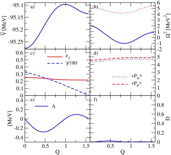
Figure 1: Large amplitude collective motion in ⁶⁸Se at $I=0$ following the lowest RPA solution at equilibrium. a) Energy along the collective path. b) The square of the lowest RPA frequencies. c) Deformation $\epsilon_{2}$ and $\gamma/180^{\circ}$. d) The dimensionless pairing operators $\left<P_{\tau}\right>$. e) The cranking parameter $\Lambda$. f) The decoupling measure, $D$.

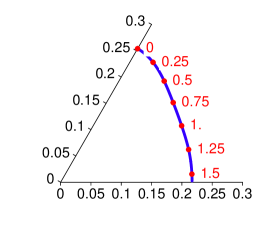
Figure 2: The deformation parameters in the $\epsilon_{2}-\gamma$ plane for ⁶⁸Se at $I=0$. Labels denote the value of the collective coordinate.

We see that the main change in the structure along the collective path is a almost linear change in the $\gamma$-deformation. The energy difference and the potential barrier between the two minima is very small, less then $200$ keV. We can therefore expect to see a large mixing of different shapes. The collective path can be mirrored around prolate and oblate minimum due to the time reversal symmetry. If we were to continue the path towards negative values of the collective coordinate $Q$ and towards larger $Q$ the potential would repeat it self in a cyclic manner. This collective path is very similar to what was recently found in Ref. KN04 . The smallness of the decoupling measure $D$ gives us reason to believe that we can obtain a very good description of the ground state in this way.

We have solved the collective Schrödinger equation, see Sec. II.4. The cyclic nature of the collective path gives condition for the radial part of the collective wave function, $U$, that $U(Q)=U(-Q)$. In Fig. 3 we can see that the ground state wave function is spread out almost uniformly along the collective path.

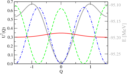
Figure 3: The wave function for the large amplitude collective motion in ⁶⁸Se at $I=0$, following the lowest RPA solution. The first three $0^{+}$ eigen functions are shown (as red solid, green dashed and blue dashed-dotted line, respectively). These wave functions are periodic around $Q=0$ and $\pm 1.57$. The grey curve (with the scale on the right-hand side) shows the collective potential energy for reference.

The ground state is thus neither prolate nor oblate, which should not surprise us since this nucleus is very $\gamma$-soft. This results in two (almost) degenerate excited states at 2 MeV excitation. This result is similar to those obtained by solving the Schrödinger equation on a circle with constant potential. There the ground state is a constant wave function, and the first two excited wave functions, $\cos\phi$ and $\sin\phi$, are degenerate, and the energy spacing only depends on the circumference of the circle.

At finite angular momentum the behaviour gets somewhat more complicated, as can be seen in Fig. 4 for $I=2$. The potential is no longer symmetric around the minimum and for positive values of the collective coordinate the path goes through the triaxial plane into a very shallow prolate minimum. The collective path then continues towards negative $\gamma$-deformation. The path ends due to an avoided crossing with a higher lying RPA mode, at which point we are no longer able to find a stable solution. This avoided crossing indicates a need to include more than one collective coordinate.

This is a generic feature of the method; whenever two modes come closely together, and thus mix strongly, we need collective coordinates for both modes to describe collective motion. Fortunately, the decoupling measure gives us a clear indication at what point of the collective surface this is the case. States with wave functions that are not sensitive to the are of large coupling should be unaffected.

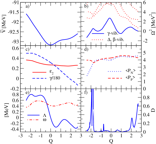
Figure 4: Large amplitude collective motion in ⁶⁸Se at $I=2$ following the lowest RPA solution at equilibrium. a) Energy along the collective path. b) The square of the lowest RPA frequencies. c) Deformation $\epsilon_{2}$ and $\gamma/180^{\circ}$. d) The dimensionless pairing operators $\left<P_{\tau}\right>$. e) The cranking parameter $\Lambda$ and the rotational frequency $\omega$. f) The decoupling measure, $D$.

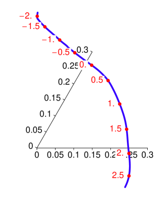
Figure 5: The deformation parameters in the $\epsilon_{2}-\gamma$ plane for ⁶⁸Se at $I=2$. Labels denote the value of the collective coordinate.

For negative $Q$ we have a linear increase in $\gamma$-deformation until $\gamma$ reaches $90^{\circ}$ and $Q\approx-1.7$, where there is a sudden change in the nature of the collective path as shown by drastic reduction in the neutron pair-field. This is accompanied with a slow increase of the $\epsilon_{2}$-deformation with $\gamma$ fixed at $90^{\circ}$. Once again the size of the decoupling measure tells us that here our single-coordinate approximation breaks down. We can thus not reliable calculate any state that has a sizable weight near $Q=-2$.

After solving the collective Schrödinger equation, we find in Fig. 6 that the wave function of the lowest $2^{+}$ state is concentrated around the oblate minimum with the tail reaching into triaxial and prolate shapes, but with little or no weight where $D$ is large.

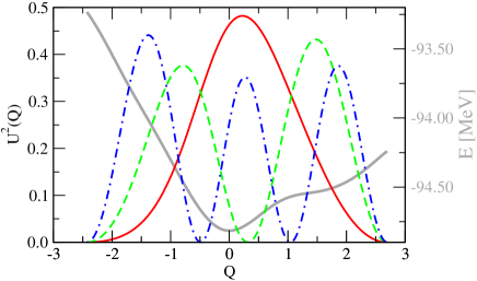
Figure 6: The wave function for the large amplitude collective motion in ⁶⁸Se at $I=2$, following the lowest RPA solution. The first three $2^{+}$ eigen functions are shown (as red solid, green dashed and blue dashed-dotted line, respectively). The grey curve (with the scale on the right-hand side) shows the collective potential energy for reference.

The first excited state has two peaks in the collective wave function corresponding to a superposition of prolate and triaxial deformations, and is less reliable due to some small weight where $D$ is large. It is only the third excited $2^{+}$ state that appears to suffer strongly from weighting where $D$ is appreciable.

Table 2: The deformation for the collective states as well as for the mean field at $I=0$ and $2$ for ⁶⁸Se.

$I_{n}$	$0_{1}$	$0_{2}$	$0_{3}$	$2_{1}$	$2_{2}$	$2_{3}$	$0_{\rm MFG}$	$2_{\rm MF}$
$\epsilon_{2}$	0.211	0.216	0.224	0.250	0.229	0.234	0.254	0.269
$\gamma$	25.6	27.5	26.1	48.1	46.5	54.5	60.0	56.4

The average deformation for the ground state and low-lying excited states are shown in Table 2 together with the mean-field deformation at $I=0$ and $2$. We conclude that mean-field and average values can be substantially different in these nuclei; also the difference between $0^{+}$ and $2^{+}$ states is interesting, with the $2^{+}$ states much closer to purely oblate than the $0^{+}$ states.

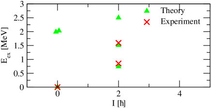
Figure 7: Calculated and experimental FB00 excitation spectrum for ⁶⁸Se as a function of angular momentum.

If we summarise these results, and compare to the experimental spectra, Fig. 7 we get some interesting results. The decoupling measure is small, and up to the lack of fine-tuning of our parameters to individual nuclei, we do expect very good results. Thus we predict a pair of almost degenerate $0^{+}$ states at about 2 MeV. The results for the $2+$ states are probably better than we could have expected: the first of these states has little sensitivity to the large decoupling measure at $Q=-2$, but the second has some. The third state must be thought of as totally unreliable.

III.2 ⁷²Kr

This nucleus has been studied in detail in Ref. AW04b . We again start by examining the $0^{+}$ states where a prolate-oblate shape coexistence has been established experimentally BM03 . We find a collective path going from the oblate minimum through a spherical energy saddle point into a prolate secondary minimum, continuing towards larger deformation, see Fig. 8. At $Q\approx 7.5$ there is an avoided crossing between the lowest RPA mode, which we are following, and two higher lying modes that are of pairing-vibrational character. This can also bee seen in Fig. 8 as a rapid increase in the decoupling measure. For negative $Q$, at large oblate deformation we see a collapse in neutron pairing, which gives a natural end to the path. Nonetheless, even at this end of the path there is an obvious avoided crossing, which suggests that the one dimensional approximation is only of limited value for this nucleus. Fortunately, the maximal value for $D$ of about 0.6 suggests, based on past experience, that the influence of any second coordinate is small.

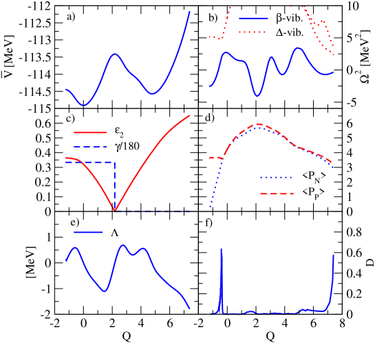
Figure 8: Large amplitude collective motion in ⁷²Kr with axial symmetry (following the $\beta$-vibration, the lowest RPA solution at equilibrium). a) Energy along the collective path. b) The square of the lowest RPA frequencies. c) Deformation $\epsilon_{2}$ and $\gamma/180^{\circ}$. d) The dimensionless pairing operators $\left<P_{\tau}\right>$. e) The cranking parameter $\Lambda$. f) The decoupling measure, $D$.

In Fig. 9 we plot the collective wave functions and can see that the ground state wave function is concentrated in the oblate minimum. The collective wave function has a substantial spread along the collective path and is skewed towards the spherical state due to the collapse in the neutron pair-field. Unfortunately, this has substantial weight in the area of the avoided crossing.

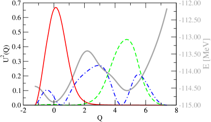
Figure 9: The wave function for the large amplitude collective motion in ⁷²Kr, following the lowest RPA solution. The first three $0^{+}$ eigen functions are shown (as red solid, green dashed and blue dashed-dotted line, respectively). These wave functions are periodic around $Q=0$ and $\pm 1.57$. The grey curve (with the scale on the right-hand side) shows the collective potential energy for reference.

The first excited state has its major component in the prolate minimum with a small component in the oblate minimum. The prolate peak in the wave function for the first excited state is broader and more symmetric then for the ground state. The third $I=0$ state is approximate spherical but has substantial oblate as well as prolate components.

At finite rotational frequency the collective path will no longer go through the spherical state, due to the effect of the rotational term (it is energetically unfavourable to generate angular momentum in a spherical state). Instead the oblate and prolate minim are connected through a path that goes through the triaxial plane. Due to problems with level crossings we have to start in both the prolate and oblate minimum, and connect these together to find the complete collective path.

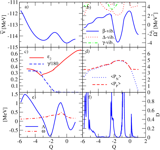
Figure 10: Large amplitude collective motion in ⁷²Kr at I=2 following the lowest RPA solution at equilibrium. a) Energy along the collective path. b) The square of the lowest RPA frequencies. c) Deformation $\epsilon_{2}$ and $\gamma/180^{\circ}$. d) The dimensionless pairing operators $\left<P_{\tau}\right>$. e) The cranking parameter $\Lambda$ and the rotational frequency $\omega$. f) The decoupling measure, $D$.

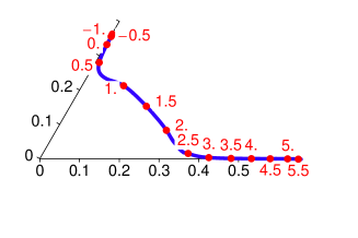
Figure 11: The deformation parameters in the $\epsilon_{2}-\gamma$ plane for ⁷²Kr at I=2. Labels denote the value of the collective coordinate.

In Fig. 10 we see that if we start in the almost oblate minimum and follow the collective path toward large oblate deformation the situation is very similar as in the non-rotating case above. We first see a decrease in the quadrupole moment but after an avoided crossing with a pairing vibration the collective path changes its nature and the collective path ends in a neutron pair-field collapse. When we follow the collective path towards smaller oblate deformation the system goes through an avoided crossing with a $\gamma$-vibrational mode.The collective path will the go into the triaxial plane and follow a path with approximately constant $\epsilon_{2}$ deformation but with decreasing $\gamma$ from just below $60$ to just above $0$. At this point the collective path goes through another avoided crossing through which the computer code cannot find a stable solution. By starting the calculation in the prolate minimum we can follow the collective path to the same avoided crossing as as we run into when starting in the oblate minimum. We can the add these two path together to get the collective path from the oblate to the prolate minimum and beyond.

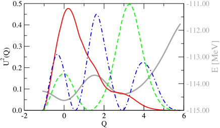
Figure 12: The wave function for the large amplitude collective motion in ⁷²Kr at I=2, following the lowest RPA solution. The first three $2^{+}$ eigen functions are shown (as red solid, green dashed and blue dashed-dotted line, respectively). These wave functions are periodic around $Q=0$ and $\pm 1.57$. The grey curve (with the scale on the right-hand side) shows the collective potential energy for reference.

When we solve the collective Schrödinger equation we get a ground state in the oblate minimum which has a substantial tail into the prolate minimum as can be seen in Fig. 12. The first excited state has its main peak in the prolate minimum with a second peak in the oblate minimum.

Table 3: The deformation for the collective states as well as for the mean field at $I=0$ and $2$ for ⁷²Kr.

$I_{n}$	$0_{1}$	$0_{2}$	$0_{3}$	$2_{1}$	$2_{2}$	$2_{3}$	$0_{\rm MF}$	$2_{\rm MF}$
$\epsilon_{2}$	0.282	0.368	0.150	0.302	0.403	0.355	0.321	0.334
$\gamma$	60.0	0.0	0.0	42.4	9.8	19.9	60.0	59.4

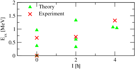
Figure 13: Calculated and experimental BM03 excitation spectrum for ⁷²Kr as a function of angular momentum.

Unfortunately, for the spectrum of this nucleus, Fig. 13, our results suggest that none of the states can be calculated reliably, due to the relatively large values of $D$ close to the minimum. Indeed comparison with the experimental data is extremely poor; a single collective coordinate is simply insufficient in this case.

III.3 ⁷⁴Kr

In ⁷⁴Kr the situation is similar to that of ⁷²Kr. For zero angular momentum the minimum has an oblate shape, as can be seen in Fig. 14.

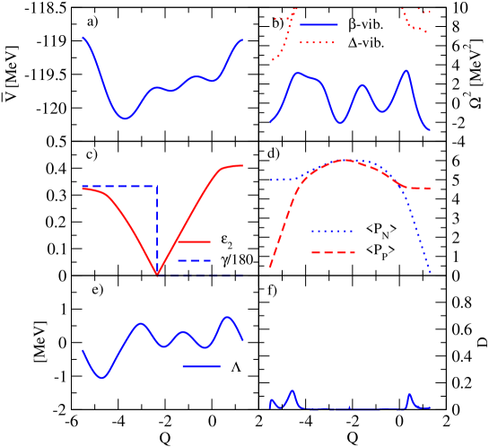
Figure 14: Large amplitude collective motion in ⁷⁴Kr at $I=0$ following the lowest RPA solution at equilibrium. a) Energy along the collective path. b) The square of the lowest RPA frequencies. c) Deformation $\epsilon_{2}$ and $\gamma/180^{\circ}$. d) The dimensionless pairing operators $\left<P_{\tau}\right>$. e) The cranking parameter $\Lambda$. f) The decoupling measure, $D$.

At large oblate deformations there is a collapse in the proton pair-field proceeded by an avoided crossing between a $\beta$-vibration and a pairing vibration that changes the direction of the collective path. Towards smaller oblate deformation the collective path goes over a spherical maximum and through two shallow prolate minima before it ends in a state with collapsed neutron pairing.

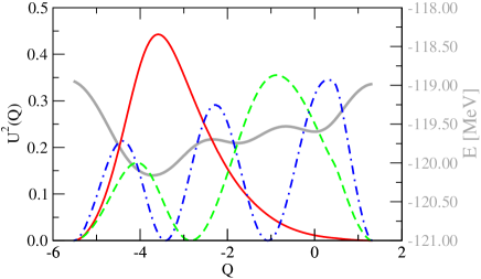
Figure 15: The wave function for the large amplitude collective motion in ⁷⁴Kr at $I=0$, following the lowest RPA solution. The first three $0^{+}$ eigen functions are shown (as red solid, green dashed and blue dashed-dotted line, respectively). These wave functions are periodic around $Q=0$ and $\pm 1.57$. The grey curve (with the scale on the right-hand side) shows the collective potential energy for reference.

The collective wave function, $U$, of the ground state is shown in Fig. 15. It shows the wave function is dominated by oblate shapes but contain a substantial tail of spherical and prolate shapes. The first excited $0^{+}$ state is a mixture of a large prolate component spread out over both the prolate minimum and a smaller oblate part. The barrier between the two prolate minima is not enough to build a collective state located mainly on each of these. The second excited $0^{+}$ state is even more complicated and contain prolate spherical and oblate shapes.

At $I=2$ we see in Fig. 16 that the prolate and oblate minimum are again connected via a path that is dominated by triaxial shapes.

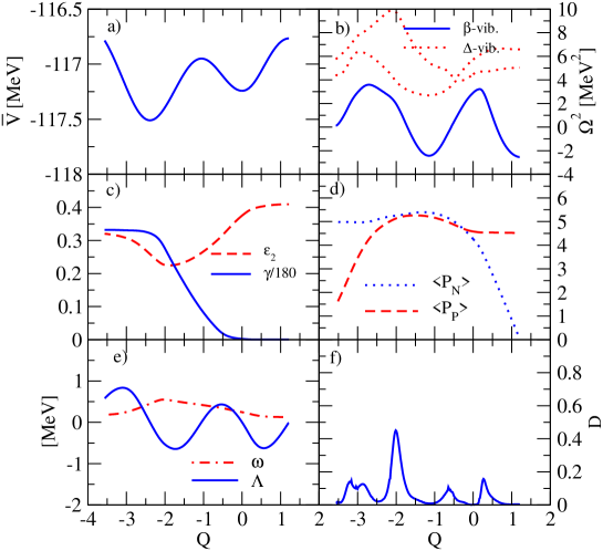
Figure 16: Large amplitude collective motion in ⁷⁴Kr at $I=2$ following the lowest RPA solution at equilibrium). a) Energy along the collective path. b) The square of the lowest RPA frequencies. c) Deformation $\epsilon_{2}$ and $\gamma/180^{\circ}$. d) The dimensionless pairing operators $\left<P_{\tau}\right>$. e) The cranking parameter $\Lambda$ and the rotational frequency $\omega$. f) The decoupling measure, $D$.

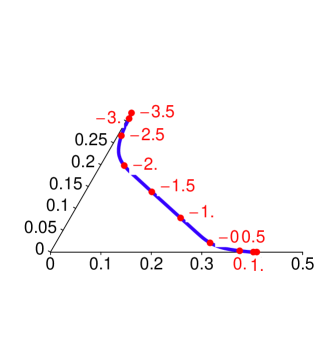
Figure 17: The deformation parameters in the $\epsilon_{2}-\gamma$ plane for ⁷⁴Kr at $I=2$. Labels denote the value of the collective coordinate.

The collective path is ended by collapses in the pair-fields at large oblate and prolate deformation. The prolate minimum we see at $I=2$ has similar deformation as the second prolate minimum at $I=0$.

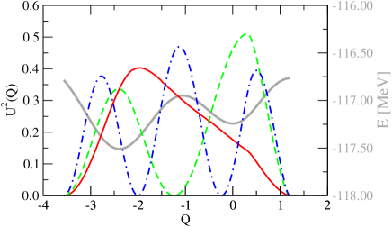
Figure 18: The wave function for the large amplitude collective motion in ⁷⁴Kr at $I=2$, following the lowest RPA solution. The first three $2^{+}$ eigen functions are shown (as red solid, green dashed and blue dashed-dotted line, respectively). These wave functions are periodic around $Q=0$ and $\pm 1.57$. The grey curve (with the scale on the right-hand side) shows the collective potential energy for reference.

The wave function of lowest $2^{+}$ state show a strongly collective nature and even though the peak is situated in the oblate minimum it has a strong admixture of triaxial and prolate shapes as can be seen in Fig. 18. The wave function of higher-lying $2^{+}$ states contain a mixture of prolate, oblate and triaxial shapes.

Table 4: The deformation for the collective states as well as for the mean field at $I=0$ and $2$ for ⁷⁴Kr.

$I_{n}$	$0_{1}$	$0_{2}$	$0_{3}$	$2_{1}$	$2_{2}$	$2_{3}$	$0_{\rm MF}$	$2_{\rm MF}$
$\epsilon_{2}$	0.125	0.135	0.098	0.304	0.320	0.314	0.213	0.259
$\gamma$	60.0	0.0	0.0	49.1	43.7	46.3	60.0	57.9

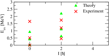
Figure 19: Calculated and experimental KC05 excitation spectrum for ⁷⁴Kr as a function of angular momentum.

In this case, Fig. 19, we expect very good results for $0^{+}$ states since $D$ is small everywhere, and good, but slightly less accurate, results for the $2^{+}$ states, since $D$ is slightly larger. Indeed, the results agree remarkably well with experimental data.

III.4 ⁷⁶Kr

In ⁷⁶Kr the collective path is almost identical to that of ⁷⁴Kr. For the unrotated case the lowest minimum has an oblate shape as can bee seen in Fig. 20.

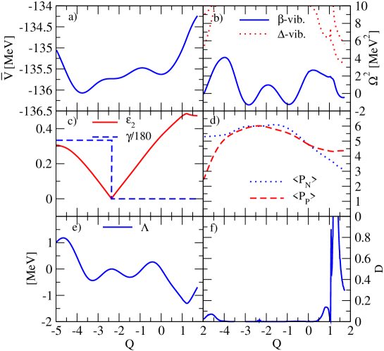
Figure 20: Large amplitude collective motion in ⁷⁶Kr at $I=0$ following the lowest RPA solution at equilibrium. a) Energy along the collective path. b) The square of the lowest RPA frequencies. c) Deformation $\epsilon_{2}$ and $\gamma/180^{\circ}$. d) The dimensionless pairing operators $\left<P_{\tau}\right>$. e) The cranking parameter $\Lambda$. f) The decoupling measure, $D$.

Towards small oblate deformation the collective path goes over a spherical maximum and through two shallow prolate minima. At each end of the collective path there is a strong reductions in the pair-fields. Due to numerical difficulties of finding a converged solution we are not able continue the calculation all the way to the pairing collapsed state.

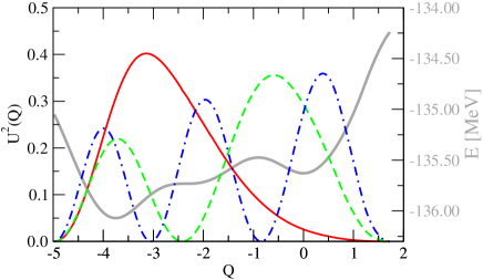
Figure 21: The wave function for the large amplitude collective motion in ⁷⁶Kr at $I=0$, following the lowest RPA solution. The first three $0^{+}$ eigen functions are shown (as red solid, green dashed and blue dashed-dotted line, respectively). These wave functions are periodic around $Q=0$ and $\pm 1.57$. The grey curve (with the scale on the right-hand side) shows the collective potential energy for reference.

The collective wave function, $U$, of the ground state is shown in Fig. 21. It shows the wave function is dominated by oblate shapes but contains a substantial tail of spherical and prolate shapes. The first excited $0^{+}$ state is a mixture of a large prolate component and a smaller oblate part. The second excited $0^{+}$ state is even more complicated and mixes prolate spherical and oblate shapes.

At $I=2$ we see in Fig. 22 that the prolate and oblate minimum are connected via a path that is dominated by triaxial shapes. The lowest minimum is not oblate at all but instead strongly triaxial ($\gamma\approx 90^{\circ}$). This is due to the fact that the collective path goes from the triaxial minimum rapidly through an oblate shaped state to a secondary prolate minimum.

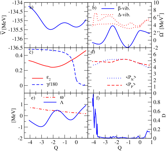
Figure 22: Large amplitude collective motion in ⁷⁶Kr at $I=2$ following the lowest RPA solution at equilibrium. a) Energy along the collective path. b) The square of the lowest RPA frequencies. c) Deformation $\epsilon_{2}$ and $\gamma/180^{\circ}$. d) The dimensionless pairing operators $\left<P_{\tau}\right>$. e) The cranking parameter $\Lambda$ and the rotational frequency $\omega$. f) The decoupling measure, $D$.

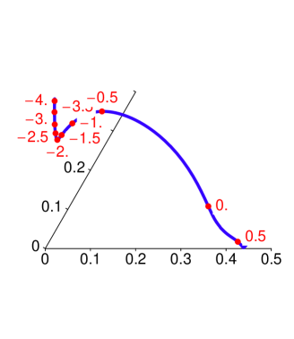
Figure 23: The deformation parameters in the $\epsilon_{2}-\gamma$ plane for ⁷⁶Kr at $I=2$. Labels denote the value of the collective coordinate.

The collective path ends due to numerical difficulties at relatively small prolate and triaxial deformations.

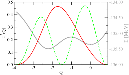
Figure 24: The wave function for the large amplitude collective motion in ⁷⁶Kr at $I=2$, following the lowest RPA solution. The first three $2^{+}$ eigen functions are shown (as red solid, green dashed and blue dashed-dotted line, respectively). These wave functions are periodic around $Q=0$ and $\pm 1.57$. The grey curve (with the scale on the right-hand side) shows the collective potential energy for reference.

The wave function of the lowest $2^{+}$ state shows a strongly collective nature and even though the peak is situated in the triaxial minimum it has a strong admixture of oblate and prolate shapes as can be seen in Fig. 18. The wave functions of higher lying $2^{+}$ states contain a mixture of prolate, oblate and triaxial shapes. The energy of the states can only be seen as an upper limit since we have not been able to follow the collective path very far in this case.

Table 5: The deformation for the collective states as well as for the mean field at $I=0$ and $2$ for ⁷⁶Kr.

$I_{n}$	$0_{1}$	$0_{2}$	$0_{3}$	$2_{1}$	$2_{2}$	$2_{3}$	$0_{\rm MF}$	$2_{\rm MF}$
$\epsilon_{2}$	0.048	0.150	0.142	0.253	0.266	0.257	0.211	0.244
$\gamma$	60.0	0.0	0.0	35.3	28.1	34.0	60.0	56.0

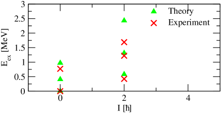
Figure 25: Calculated and experimental KC05 excitation spectrum for ⁷⁶Kr as a function of angular momentum.

Thus, see Fig. 25, the energies first two $0^{+}$ states should be reliable, but the third is somewhat more doubtful, due to the peak in $D$ at $Q=-1$. The $2^{+}$ states are of similar quality. It is thus surprising that theory predicts a low-lying second $0+$-state that has not been observed in experiment!

III.5 ⁷⁸Kr

For ⁷⁸Kr we have behaviour similar to ⁶⁸Se in that the lowest RPA mode in the minimum is a $\gamma$-vibration. The prolate and oblate minimum are therefore connected through triaxial states.

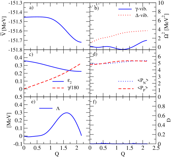
Figure 26: Large amplitude collective motion in ⁷⁸Kr at $I=0$ following the lowest RPA solution at equilibrium. a) Energy along the collective path. b) The square of the lowest RPA frequencies. c) Deformation $\epsilon_{2}$ and $\gamma/180^{\circ}$. d) The dimensionless pairing operators $\left<P_{\tau}\right>$. e) The cranking parameter $\Lambda$. f) The decoupling measure, $D$.

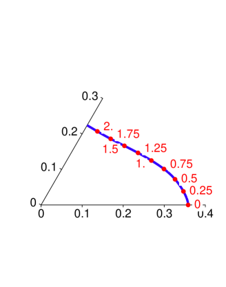
Figure 27: The deformation parameters in the $\epsilon_{2}-\gamma$ plane for ⁷⁸Kr at $I=0$. Labels denote the value of the collective coordinate.

The potential barrier between the oblate minimum, which is lowest in energy, and the secondary prolate minimum is only $250$ keV as can be seen in Fig. 26. In Fig. 28 we see that this leads to a situation very similar to that of ⁶⁸Se where the collective ground state wave function, $U$, represent a approximately equal mixture of all possible triaxial shapes with an approximately constant $\epsilon_{2}$-deformation and pair-fields.

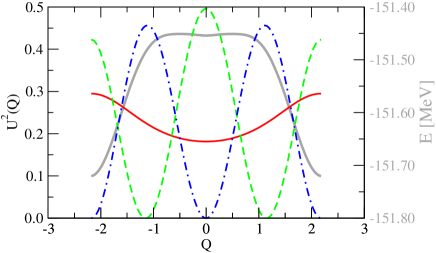
Figure 28: The wave function for the large amplitude collective motion in ⁷⁸Kr at $I=0$, following the lowest RPA solution. The first three $0^{+}$ eigen functions are shown (as red solid, green dashed and blue dashed-dotted line, respectively). These wave functions are periodic around $Q=0$ and $\pm 1.57$. The grey curve (with the scale on the right-hand side) shows the collective potential energy for reference.

We also see that the excitation spectrum in ⁷⁸Kr is very similar to that of ⁶⁸Se. We have two almost degenerate excited $0^{+}$ states that can be interpreted as rotational excitation (in $\gamma$). The fact these excited states lie at $1$ MeV in ⁷⁸Kr compared to $2$ MeV ⁶⁸Se in simply due to the longer ’distance’ between the prolate and the oblate minimum in ⁷⁸Kr.

At at finite rotational frequency ($I=2$) we have a slightly different picture for ⁷⁸Kr. The lowest RPA solution in the almost axial prolate minimum is a neutron paring vibration. This leads to a rapid collapse of the neutron pair-field at small negative values of the collective coordinate, as can be seen in Fig. 29.

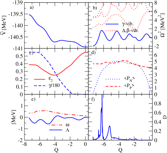
Figure 29: Large amplitude collective motion in ⁷⁸Kr at $I=2$ following the lowest RPA solution at equilibrium). a) Energy along the collective path. b) The square of the lowest RPA frequencies. c) Deformation $\epsilon_{2}$ and $\gamma/180^{\circ}$. d) The dimensionless pairing operators $\left<P_{\tau}\right>$. e) The cranking parameter $\Lambda$ and the rotational frequency $\omega$. f) The decoupling measure, $D$.

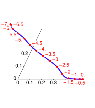
Figure 30: The deformation parameters in the $\epsilon_{2}-\gamma$ plane for ⁷⁸Kr at $I=2$. Labels denote the value of the collective coordinate.

At positive values of $Q$ there is an increase in the neutron pair-field and a decrease in the $\epsilon_{2}$-deformation. At $Q\approx 1.8$ there is an avoided crossing that changes the direction of the collective path into the triaxial plane. The path goes towards larger $\gamma$ until we reach a almost oblate state with $\gamma\approx 60$ and $Q\approx 4.1$. The collective path passes through this secondary minimum in to triaxial plane. At $Q\approx 6.2$ we have a second avoided crossing and a transition into a path with decreasing neutron pair-field which leads to a neutron paring collapse at $Q\approx 7.4$. Due to the shallowness of the barrier between the prolate and oblate sates the ground state wave function has a substantial tail stretching out of the prolate minimum through the triaxial plane into the oblate secondary minimum, see Fig. 31.

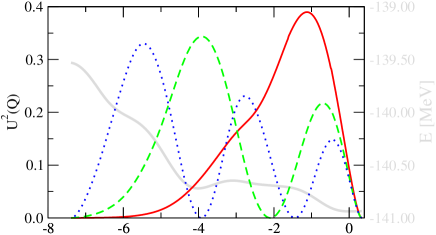
Figure 31: The wave function for the large amplitude collective motion in ⁷⁸Kr at $I=2$, following the lowest RPA solution. The first three $2^{+}$ eigen functions are shown (as red solid, green dashed and blue dashed-dotted line, respectively). These wave functions are periodic around $Q=0$ and $\pm 1.57$. The grey curve (with the scale on the right-hand side) shows the collective potential energy for reference.

There are another two low lying $2^{+}$ states. The first of these is dominated by a oblate component but has also a sizable prolate part.

Table 6: The deformation for the collective states as well as for the mean field at $I=0$ and $2$ for ⁷⁸Kr.

$I_{n}$	$0_{1}$	$0_{2}$	$0_{3}$	$2_{1}$	$2_{2}$	$2_{3}$	$0_{\rm MF}$	$2_{\rm MF}$
$\epsilon_{2}$	0.266	0.276	0.278	0.397	0.286	0.266	0.224	0.548
$\gamma$	26.3	20.8	24.2	7.1	32.3	52.5	60.0	60.0

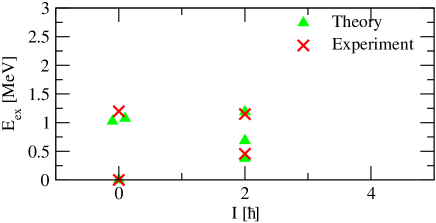
Figure 32: Calculated and experimental KC05 excitation spectrum for ⁷⁸Kr as a function of angular momentum.

In this case, Fig. 32, the spectrum is somewhat similar to ⁶⁸Se, due to the extreme $\gamma$-soft character of the $0^{+}$ states. In this case one of the two excited $0^{+}$ states has actually been detected. The data obtained in these difficult experiments are not of sufficient quality to rule out that this is actually a narrow doublet. The data on $2^{+}$ states is also compatible with an additional low-lying $2^{+}$ that has not been seen in experiment.

IV Conclusions

We have extended the method of calculating the self-consistent collective path presented in DK00 ; AW04 to include constraints on angular momentum and particle number and implemented it for the quadrupole+pairing Hamiltonian BK68 . The method consists of finding a series of points fulfilling the force equation, where the local direction of the collective path is determined in each point by the local normal modes. The local RPA equations and the force equation are solved in a double iterative process with constraints on angular momentum and particle numbers along the collective path. The method allows us to determine the collective coordinate from the Hamiltonian without having to assume a priori which are the relevant degrees of freedom.

The results confirm the importance of pairing collapsed states for the collective path as suggested in AW04 . We have also seen a very different behaviour of the collective path between the prolate and oblate minimum depending on $N$ and $Z$ as well as weather we are looking at the ground state or an rotating state. Without rotation the path either goes through a spherical maximum or through the triaxial plane. In the rotating case the two minima are always connected via the triaxial plane. This difference comes because at finite angular momentum the system tries to avoid the spherical state because the cost of generating angular momentum gets larger as the deformation gets smaller. This effect would not have been seen so clearly if the calculation was done at constant rotational frequency instead of at constant angular momentum. The difference would be less pronounced if we would have allowed for more the one collective coordinate.

The results shed new light on the behaviour of these nuclei, and make predictions which can be of importance experimentally, especially the extreme $\gamma$-soft nature of ⁶⁸Se and ⁷²Kr at low angular momentum. Discovery of the predicted doublets of excited $0^{+}$ states would shed light on the nature of shape mixing in these nuclei. It is extremely encouraging that where we expect our method to be reliable (i.e., where $D$ is small) we get a good correspondence with experiment, and where we have a poor correspondence, decoupling is poor. We have also seen that the nature of shape-mixing and shape-coexistence is indeed quite complicated in the group of nuclei discussed here, and changes rapidly along the isotope chain. The picture seems to be less systematic than discussed in the literature. Mixing is large in all cases.

In this paper we have implemented a method to find the adiabatic self-consistent collective path for a nuclei. A technique to truncate the basis in which the RPA equations are solved has been improved and a good agreement between the full and truncated RPA is found. To solve the RPA equations in a limited basis has proven to be a useful and practical way of calculating the collective path within the local harmonic approximation. It remains to be investigated how we can include the covariant terms in the RPA in a suitable approximation.

Appendix A Comparison with Matsuo et al.

In the work of Matsuo at al., the adiabatic large amplitude collective motion (ALACM) is described in what looks superficially entirely different than our method. Nonetheless, the final results are so similar that there must be similarities. It is therefore useful to analyse the problem in various ways and compare the two methods in a unified notation. The key difference is the direct formulation in terms of mean field equations by Matsuo et al., and our insistance on classical mechanics.

Let us initially look at one way to derive the localised harmonic approach in our notation, which we shall than tie closely to the work in Ref. MN00 . We expand the collective energy (actually the generalised density matrix) to second order in small fluctuations, thus obtaining a Hamiltonian. The method is based on “removing the linear terms”, which means that at any point $P$, which is really a time-even HFB state, along the collective path, we approximate the Hamiltonian by the quadratic form

$${\cal H}=\frac{1}{2}\pi_{\alpha}B^{\alpha\beta}(P)\pi_{\beta}+V(P)+V_{,\alpha}(P)\xi^{\alpha}+\frac{1}{2}V_{,\alpha\beta}(P)\xi^{\alpha}\xi^{\beta}\quad.$$ (19)

In order to look at the local fluctuations, we need to remove the term linear in $\xi$. We first modify $\cal H$ by constraints (such as those for particle number and angular momentum; we shall include particle number only here). With the Lagrange multiplier term $\mu(N-N_{0})$ we really have

$${\cal H}-\lambda N=\frac{1}{2}\pi_{\alpha}(B^{\alpha\beta}-\mu\partial_{\pi_{\alpha}}\partial_{\pi_{\beta}}N)(q_{0})\pi_{\beta}+V(q_{0})+(V_{,\alpha}-\mu N_{,\alpha})(q_{0})\xi^{\alpha}+\frac{1}{2}(V_{,\alpha\beta}(q_{0})-\mu N_{,\alpha\beta}-\mu_{,\alpha}N_{,\beta}-\mu_{,\beta}N_{,\alpha})\xi^{\alpha}\xi^{\beta}\quad.$$ (20)

In order to remove the linear term, we require that it can be removed by purely collective term, i.e., a term of the form $\lambda Q$, with $\lambda$ defined at the collective point $Q=q_{0}$. We thus require that

$$V_{,\alpha}-\mu N_{,\alpha}=\lambda f_{,\alpha}\quad,$$ (21)

with $f_{,\alpha}=Q_{,\alpha}$, and we get the quadratic Hamiltonian (where we have absorbed the terms arising from expanding $\langle H-\mu N\rangle$ for fixed $\mu$ in $B$ and $V$, and denoted the compound object by a tilde). The Hamiltonian with the constraint $\lambda Q$ becomes

$${\cal H}^{\prime}=\frac{1}{2}\pi_{\alpha}({\tilde{B}}^{\alpha\beta})\pi_{\beta}+V+\frac{1}{2}({\tilde{V}}_{,\alpha\beta}-\mu_{,\alpha}N_{,\beta}-\mu_{,\beta}N_{,\alpha}-\lambda f_{,\alpha\beta})\xi^{\alpha}\xi^{\beta}\quad.$$ (22)

It has been argued coherently in Ref. DK00 that the final term is equivalent to the covariant term in the derivative

$$\Gamma_{\alpha\beta}^{\gamma}V_{,\gamma},$$

and we are now left with a simple normal mode problem, which is of course nothing more than the usual RPA. The self-consistency is now obtained by requiring $f$ to be one of the normal mode directions. We thus can write the RPA as two coupled equation (or as a single one)

$${\tilde{B}}^{\alpha\beta}f_{,\beta} =\bar{B}g^{\alpha}\quad,$$ (23)

$$({\tilde{V}}_{,\alpha\beta}-\mu_{,\alpha}N_{,\beta}-\mu_{,\beta}N_{,\alpha}-\lambda f_{,\alpha\beta})g^{\beta} =\bar{V}_{;QQ}f_{\alpha}\quad.$$ (24)

Let us now compare this approach with that of KN03 ; KN05 , which is cast in the form of a set of variational equations. If we take into account that to first order the time-even part of fluctuations is $\xi^{\alpha}/\sqrt{2}$, with $\pi_{\alpha}/\sqrt{2}$ the time-odd part, it is relatively straight-forward to show that the three equations (2.34-2.36) in ref. MN00 would be written as
(note:

• we use $\mu$ where Ref. MN00 uses $\lambda$;

• in our notation $\lambda=\bar{V}(Q)_{,Q}$, where we use the bar to denote a collective quantity, as distinguished from the quantity defined in the full space DK00 .

• $f_{,\alpha}=\sqrt{2}\delta\langle\hat{Q}\rangle$.

• $g^{,\alpha}=\sqrt{2}\delta\langle\hat{P}\rangle$.)

$$V_{,\alpha}-\mu N_{,\alpha}-\lambda f_{,\alpha} =0\quad,$$ (25)

$${\tilde{B}}^{\alpha\beta}f_{,\beta}-\bar{B}g^{\alpha} =0\quad,$$ (26)

$$\frac{1}{2}\left[f_{,\alpha}{\tilde{B}}^{\alpha\beta}f_{,\beta}\right]_{,\gamma}-\bar{B}\frac{1}{2}\left[f_{,\gamma\beta}g^{\beta}+\bar{\Gamma}f_{,\gamma}\right] =0\quad.$$ (27)

The first of these relations is the one that removes the linear term, as above. The second defines the collective momentum, and finally the last equation defines the affine connection $\bar{\Gamma}$,

$$\bar{B}\bar{\Gamma}=\frac{1}{2}\tilde{B}^{\alpha\beta}_{,\gamma}f_{,\alpha}f_{,\beta}g^{\gamma}\quad.$$ (28)

Exactly the same relation can be found in Ref. DK00 . Whereas in the local fluctuation approach we construct fluctuations in all directions, the work in Ref. MN00 differentiates only with respect to the collective coordinates. This implies an assumption about block-diagonality of $\Gamma$ that is justified for exact decoupling. We get for Eq. (3.1) in Ref. MN00 ,

$$(V_{,\alpha\beta}-\mu N_{,\alpha\beta})g^{\beta}-\bar{V}_{;QQ}f_{,\alpha}-\bar{V}_{,Q}\left[f_{,\alpha\beta}g^{\beta}+\bar{\Gamma}f_{,\alpha}\right]-\mu_{,Q}N_{,\alpha}=0$$ (29)

This can also be rewritten as (using $\bar{V}_{,Q}=\lambda$ and $\mu_{,Q}=\mu_{,\alpha}g^{\alpha}$)

$$(V_{,\alpha\beta}-\mu N_{,\alpha\beta}-\lambda f_{,\alpha\beta}-\mu_{,\beta}N_{,\alpha})g^{\beta}=\lambda_{,Q}f_{,\alpha},$$ (30)

which is almost what we would argue constitutes the covariant RPA equation, cf. Eqs. (24). There is a very subtle difference, and that is due to the fact that the matrix on the left-hand-side in 30 is not symmetric under interchange of the labels $\alpha$ and $\beta$. The term that is missing as compared to the local fluctuation approach discussed above is $-\mu_{,\alpha}N_{,\beta}g^{\beta}=-\mu_{,\alpha}N_{,Q}$. The absence comes from treating $\mu=\mu(Q)$ in the approach of Ref. MN00 as an external parameter, whereas, in the language of that paper, we take $\mu(\langle\hat{Q}\rangle)$, i.e., as a function of the mean-field expectation value of $\hat{Q}$, which clearly changes with the mean field, and thus leads to the additional term.

We believe that symmetry of all the RPA equations is crucial, and thus are worried about such missing terms. Of course, in the current paper we have grossly neglected all covariant terms, which clearly is also objectionable. We do wonder, however, if this lack of symmetry is what leads to the $K$-symmetry non-preserving path seen in Ref. KN05 . Without angular momentum constraints, the local RPA for axial states will always have eigenvalues with definite $\Delta K$, i.e., to change from following a $\beta$ to a $\gamma$ vibration, we must have a real rather than avoided crossing in the RPA.

The further developments in Ref. MN00 are also interesting; they correspond to trying to evaluate $f_{,\alpha\beta}$, the variation of the collective coordinate operator. Even if it were a one body operator, as we tacitly assume, and is necessary for exact decoupling, the equations only fix the 2 quasi-particle part of this operator, i.e., terms going like $c^{\dagger}c^{\dagger}$ or $cc$. The approximation made in Ref. MN00 is to assume that the $c^{\dagger}c$ matrix elements are identically zero. This is the only closed form approximation that can be made, but must be dealt with carefully: it would fail for some problems with exact decoupling. In an approach that uses a basis of operators, one could evaluate such terms by the relevant matrix elements of the operators, multiplied by their coefficients DK00 .

We thus conclude that the underlying expressions in our approach and that set out in Ref. MN00 are almost, and should be completely, identical. We are concerned about the missing term in the potential expansion.

References

- (1) N. Bohr and F. Kalckar, Mat. Fys. Medd. Dan. Vid. Selsk. 14, no. 10 (1937).
- (2) P. Ring and P. Schuck, The Nuclear Many-Body Problem, (Springer, New York, 1980)
- (3) G. Do Dang, A. Klein and N.R. Walet, Phys. Rep. 335, 93 (2000)
- (4) Tunnelling in complex systems edited by S. Tomsovic, (World Scientific, Singapore; London, 1998)
- (5) D. Almehed and N.R. Walet, Phys. Rev C 69, 024302 (2004)
- (6) M. Matsuo, T. Nakatsukasa, and K. Matsuyanagi, Prog. Theor. Phys. 103, 959 (2000).
- (7) M. Kobayasi, T. Nakatsukasa, M. Matsuo and K. Matsuyanagi, Prog. Theor. Phys. 110, 65 (2003), nucl-th/0304051
- (8) M. Kobayasi, T. Nakatsukasa, M. Matsuo and K. Matsuyanagi, Prog. Theor. Phys. 112, 363 (2004).
- (9) M. Kobayasi, T. Nakatsukasa, M. Matsuo and K. Matsuyanagi, Prog. Theor. Phys. 113, 129 (2005), nucl-th/0412062.
- (10) T. Nakatsukasa, N.R. Walet and G. Do Dang, Phys. Rev. C 61, 014302 (1999)
- (11) D. Almehed and N.R. Walet, Acta Phys. Pol. B 34, 2227(c) (2003)
- (12) D. Almehed and N.R. Walet, Phys. Lett. B 604, 163 (2004)
- (13) S.M. Fisher, D.P. Balamuth, P.A. Hausladen, C.J. Lister, M.P. Carpenter, D.Seweryniak, and J. Schwartz, Phys. Rev. Lett. 84, 4064 (2000)
- (14) E. Bouchez et al., Phys. Rev. Lett. 90, 082502 (2003)
- (15) C. Chandler et al., Phys. Rev. C56, R2924 (1997); ibid. 61 044309 (2000)
- (16) F. Becker et al., Eur. Phys. J. A 4, 103 (1999)
- (17) W. Korten et al., Nucl. Phys. A 752, 255c (2005)
- (18) R. Abraham, J.E. Marsden and T. Ratiu, Manifolds, Tensor Analysis, and Applications (Second Edition) (Springer-Verlag, New York, 1988)
- (19) T. Young, Ph.D thesis, UMIST, 2004; T. Young and N. R. Walet, J. Phys. G: Nucl. Part. Phys. 31, 1067-1081 (2005).
- (20) M. Barranger and K. Kumar, Nuc. Phys. A110, 490 (1968)
- (21) S.G. Nilsson and I. Ragnarsson, Shapes and Shells in Nuclear Structure (Cambridge University Press) (1995)
- (22) D. Almehed and N.R. Walet, J. Phys. G: Nucl. Part. Phys., 31 S1523 (2005)