A statistical model analysis of yields and fluctuations in 200 GeV Au-Au collisions

Abstract

We show that the simultaneous measurement of yields and fluctuations is capable of falsifying and constraining the statistical hadronization model. We show how such a measurement can test for chemical non-equilibrium, and distinguish between a high temperature chemically equilibrated freeze-out from a supercooled freeze-out with an over-saturated phase space. We perform a fit, and show that both yields and fluctuations measured at RHIC 200 GeV can be accounted for within the second scenario, with both the light and strange quark phase space saturated significantly above detailed balance. We point to the simultaneous fit of the $K/\pi$ fluctuation and the $K^{*}/K^{-}$ ratio as evidence that the effect of hadronic re-interactions after freeze-out is small.

The statistical hadronization model (SHM) Fer50 ; Pom51 ; Lan53 has been extensively applied to the study of soft particle production in hadronic systems. When it includes the full spectrum of hadronic resonances Hag65 , the SHM can describe quantitatively the abundances of all light and strange hadrons produced in heavy ion collisions.

The ability of the SHM to describe not just averages, but event-by-event multiplicity fluctuations has however not been widely investigated, and its applicability is currently a matter of controversy. Event-by-event particle fluctuations have elicited theoretical fluct2 ; jeonkochratios ; fluct4 ; fluct6 and experimental interest starfluct2 ; phefluct , both as a consistency check for existing models  fluct2 ; jeonkochratios , as a test of hadron gas equilibration and the presence of resonances fluct2 , and as a way to search for new physics fluct4 .

This study investigates weather the SHM can explain both yields and fluctuations with the same parameters. We illustrate the use of both yields and fluctuations as a probe capable of differentiating between freeze-out scenarios. We then perform a fit to preliminary 200 GeV RHIC experimental data, and discuss the results in the context of chemical (non)equilibrium within the RHIC system, the freeze-out temperature and the presence (or absence) of hadronic reinteraction after freeze-out.

The statistical hadronization model assumes that particles are produced according to a probability determined by their phase space density. The first and second cumulants of this probability distribution give, respectively, the average value (over all events) of the desired observable, and its event-by-event fluctuation.

Conserved quantities can be treated in several ways, appropriate to different experimental situations: If the totality of the system is observed, than conserved quantities can not fluctuate. If a small fraction equilibrated with the rest of the system ( the “bath”) is observed, than conserved quantities will fluctuate, event-by-event. Rigorous conservation is known as the Microcanonical ensemble, while allowing energy and other conserved quantities to fluctuate between the system and the bath leads, respectively, to the Canonical and Grand Canonical (GC) ensembles. As shown recently nogc2 , all fluctuations are ensemble-specific even in the thermodynamic limit.

In this work, we use the GC ensemble, implemented in a publicly-available software package share to calculate fluctuations and yields. We motivate this choice by the fact that RHIC experiments observe the mid-rapidity slice of the system, comprising roughly 1/8 of the total multiplicity, an appropriate fraction for a GC prescription. Boost invariance, a good symmetry around mid-rapidity, links this rapidity slice with a sector in configuration space. If the system observed at RHIC is a nearly ideal fluid, the matter created in this space should be in equilibrium, grand-canonically, with the unobserved regions. If freeze-out temperature throughout observed space is approximately constant, the GC ensemble should be able to describe both yields and fluctuations cleymans ; prlfluct .

The final state yield of particle $i$ is computed by adding the direct yield and all resonance decay feed-downs.

$$\langle N_{i}\rangle_{\rm total} = \langle N_{i}\rangle+\sum_{{\rm all}\;j\rightarrow i}B_{j\rightarrow i}\langle N_{j}\rangle$$ (1)

Here $\left\langle N_{i}\right\rangle$ is the ensemble average of the $i$-th particle (resonance) multiplicity at chemical freeze-out and $B_{j\to i}$ is the branching ratio of the $j\rightarrow i$ decay. The fluctuation $\left\langle\Delta X^{2}\right\rangle=\left\langle X^{2}\right\rangle-\left\langle X\right\rangle^{2}$ also has two parts

$$\left\langle\Delta N_{j\to i}^{2}\right\rangle = B_{j\to i}(1-B_{j\to i})\left\langle N_{j}\right\rangle+B_{j\to i}^{2}\left\langle\Delta N_{j}^{2}\right\rangle\phantom{.....}$$ (2)

assuming no primordial correlation between $i$ and $j$.

The fluctuation of a ratio $N_{1}/N_{2}$ (a useful experimental observable, since volume fluctuations cancel out event-by-event) can be computed from the fluctuation of the denominator and the numerator jeonkochratios ($\sigma_{X}^{2}=\left\langle\Delta X^{2}\right\rangle/\left\langle X\right\rangle$):

$$\sigma_{N_{1}/N_{2}}^{2} = \frac{1}{\left\langle N_{2}\right\rangle}\left(D_{11}+D_{22}-2D_{12}\right)$$ (3)

$$D_{11} = {\left\langle N_{2}\right\rangle\over\left\langle N_{1}\right\rangle}\,F_{1}\phantom{A},\phantom{A}D_{22}=F_{2}$$ (4)

$$D_{12} = \sum_{j\rightarrow 1,2}B_{j\rightarrow 1,2}{{\left\langle N_{j}\right\rangle}\over{\left\langle N_{1}\right\rangle}}$$ (5)

$$F_{i} = \left(\frac{\left\langle\Delta N_{i}^{2}\right\rangle_{\rm direct}}{\left\langle N_{i}\right\rangle}+\sum_{j\rightarrow i}\left\langle N_{j\rightarrow i}^{2}\right\rangle\frac{\left\langle N_{j\rightarrow i}\right\rangle}{\left\langle N_{i}\right\rangle}\right)\phantom{......}$$ (6)

Note the appearance of a negative correlation term $D_{12}$, which arises due to the correlation between $N_{1}$ and $N_{2}$ stemming from a common resonance feed-down ($\Delta\rightarrow p\pi$ will be a source of correlation between $N_{p}$ and $N_{\pi}$).

The average yields and fluctuations of hadrons themselves can be calculated by a textbook method given a grand canonical description of the phase space; For a hadron with an energy $E_{p}=\sqrt{p^{2}+m^{2}}$, the average number, and event by event fluctuation will be given by

$$\langle N_{i}\rangle = gV\int{d^{3}p\over(2\pi)^{3}}\,{1\over\lambda_{i}^{-1}e^{E_{p}\beta}\pm 1}$$ (7)

$$\langle\Delta N_{i}^{2}\rangle = \lambda_{i}{\partial\over\partial\lambda_{i}}\langle N_{i}\rangle$$ (8)

where the upper sign is for Fermions and the lower sign is for Bosons. Here $\lambda_{i}$ is the fugacity of particle $i$, see Eq. (10). These formulae can be efficiently calculated through a Bessel function expansion Fer50 ; share .

Note that the series start diverging at $\lambda_{i}\rightarrow e^{m_{i}/T}$, and that for fluctuations the higher order terms in the expansion are always more significant than for yields: for $\lambda_{i}e^{m_{i}/T}=1-\epsilon$

$$\lim_{\epsilon\rightarrow 0}\left\langle N_{i}\right\rangle\propto\epsilon^{-1},\qquad\lim_{\epsilon\rightarrow 0}\left\langle\Delta N_{i}^{2}\right\rangle\propto\epsilon^{-2}.$$ (9)

The parameter $\lambda_{i}$ corresponds to the particle fugacity, related to the chemical potential by $\lambda_{i}=e^{\mu_{i}/T}$. Provided the law of mass action holds, it should be given by the product of charge fugacities (flavor, isospin etc.). It is then convenient to parametrize it in terms of equilibrium fugacities $\lambda_{i}^{\mathrm{eq}}$ and phase space occupancies $\gamma_{i}$. For a hadron with $q(\overline{q})$ light quarks, $s(\overline{s})$ strange quarks and isospin $I_{3}$ the fugacity is then

$$\lambda_{i}=\lambda_{i}^{\mathrm{eq}}\gamma_{q}^{q+\overline{q}}\gamma_{s}^{s+\overline{s}}\phantom{A},\phantom{A}\lambda_{i}^{\mathrm{eq}}=\lambda_{q}^{q-\overline{q}}\lambda_{s}^{s-\overline{s}}\lambda_{I_{3}}^{I_{3}}$$ (10)

If the system is in chemical equilibrium then detailed balance requires that $\gamma_{q}=\gamma_{s}=1$. In an expanding system, however, the condition of chemical equilibrium no longer holds. Kinetically, this occurs because collective expansion and cooling will make it impossible for endothermic and exothermic reactions, or for creation and destruction reactions of a rare particle, to be balanced. Provided the system remains in local thermal equilibrium, $\lambda_{i}$ can still be used as a Lagrange multiplier for the particle density, and the first and second cumulants can be calculated from the partition function the usual way jansbook ; chemistrywebsite . However, in this case in general $\gamma_{q}\neq 1,\gamma_{s}\neq 1$.

Figure 1: Fit of preliminary 200 GeV data, including the $K^{\pm}/\pi^{\pm}$ fluctuations and the $K^{*}(892)$ and $\Lambda^{*}(1520)$ resonance

This picture becomes particularly appropriate if the expanding system undergoes a fast phase transition from a QGP to a hadron gas. In this case, chemical non-equilibrium sudden and super-cooling csorgo can arise due to entropy conservation: By dropping the hadronization temperature to $\sim 140MeV$ and oversaturating the hadronic phase space above equilibrium ($\gamma_{q}\sim 1.5,\gamma_{s}\sim 2$), it is possible to match the entropy of a hadron gas with that of a system of nearly massless partons sudden .

Fits to experimental data at both SPS observing and RHIC energies Rafelski:2003ju indeed support these values of $\gamma_{q,s}$ when these parameters are fitted. Moreover, best fit $\gamma_{q,s}>1$ arises for a critical energy gammaq_energy (corresponding to the energy of the $K/\pi$ “horn” horn ) and system size gammaq_size , just as expected from the interpretation of $\gamma_{q}$ as a manifestation of a phase transition. However, the fits performed in gammaq_energy have not been able to rule out equilibrium models (at SPS and RHIC the difference in statistical significance between equilibrium and non-equilibrium is $\sim 20\%$).

In the absence of contrary evidence, equilibrium models are usually preferred for their smaller number of free parameters barannikova ; bdm . Equilibrium freeze-out temperature varies between fits, ranging from 155 gammaq_energy to 177 bdm MeV.

Both scenarios are physically reasonable, can describe the data, and would be instrumental in our understanding of hadronic matter if proven correct. In particular, the HBT puzzle suggests we lack understanding of the last stages of the fireball evolution. Non-equilibrium is useful in this respect, since it affects both system volume bari ; gammaq_energy and emission time csorgo .

The reason both equilibrium and non-equilibrium are compatible with data is that in a fit to yields the non-equilibrium phase space occupancies $\gamma_{s}$ and $\gamma_{q}$ correlate with freeze-out temperature gammaq_energy , making a distinction between a $T=170$ MeV equilibrated freeze-out ($\gamma_{q}=1,\gamma_{s}\leq 1$) scenario and a supercooled scenario where $\gamma_{q,s}>1$ problematic.

A related ambiguity is the difference between chemical freeze-out (where particle abundances are fixed) and thermal freeze-out (where particles cease to interact). Equilibrium models generally assume a long phase between these two points, which would alter considerably the multiplicity of directly detectable resonances. In a Non-equilibrium supercooled freeze-out, on the other hand, it is natural to assume that particle interaction after emission is negligible. Once again, a reliable way to probe the extent of the reinteraction would be instrumental for our understanding of how the fireball produced in heavy ion collisions breaks up.

We have recently shown prlfluct that event-by-event fluctuations can be used to solve both of the dilemmas discussed above. From the equations in the previous section, it is clear that the dependence of fluctuations of $T$ and $\gamma_{q}$ is different, allowing us to decouple these two variables. A higher temperature tends to decrease fluctuations w.r.t. the Poisson value expected from Boltzmann statistics ($\sigma=1$) , since it introduces greater correlations due to an increased contribution of resonances ($D_{12}$ in Eq. 3) . Vice-versa, increasing $\gamma_{q}$ will rapidly increase fluctuations of quantities related to pions, due to the fact that at $\gamma_{q}>1$ $\lambda_{\pi}$ rapidly approaches $e^{m_{\pi}/T}$, giving fluctuations an extra boost w.r.t. yields as per Eq. 9

In addition, comparing fluctuations to directly detected resonances probes the interval between chemical and thermal freeze-out. Consider, for example, the $K^{+}/\pi^{-}$ fluctuation. The top and the bottom terms in this ratio are linked by a large correlation term due to the $K^{*0}(892)$ decay. This correlation probes the $K^{*0}$ abundance at chemical freeze-out, since subsequent rescattering/regeneration does not alter the fact that the $K^{*0}$ decay produced a $\pi^{+}$ and a $K^{-}$. On the other hand, a direct measurement of the $K^{*}/K^{-}$ ratio through invariant mass reconstruction measures the $K^{*}$ abundance at thermal freeze-out, after all rescattering. Hence, comparing the $K/\pi$ fluctuation to the $K^{*}/K^{-}$ ratio provides a gauge for effect of the hadronic reinteraction period on particle abundances. In particular, a sudden freeze-out model should describe both with the same parameters.

The main experimental problem with fluctuation measurements is the vulnerability to effects resulting from limited detector acceptance. This difficulty can be lessened, to some extent, by considering “dynamical” fluctuations, obtained by subtracting a “static” contribution which should be purely Poisson in an ideal detector. The exact nature of the subtraction varies from collaboration to collaboration, for example supriya using

$$\sigma^{dyn}=\sqrt{\sigma^{2}-\sigma_{stat}^{2}}$$ (11)

$\sigma_{stat}$, usually obtained through a Mixed event approach pruneau , includes a baseline Poisson component, which for a ratio $N_{1}/N_{2}$ can be modeled as

$$\sigma_{stat}^{2}=\frac{1}{\left\langle N_{1}\right\rangle}+\frac{1}{\left\langle N_{2}\right\rangle}$$ (12)

as well as a contribution from detector efficiency and kinematic cuts. Provided certain assumptions for the detector response function hold (see appendix A of pruneau ), subtracting $\sigma_{stat}$ from $\sigma$ should yield a “robust” detector-independent observable.

When using measured $\sigma^{dyn}$s in fits to experimental data, the data-sample should include $\sigma^{dyn}$, particle yields (which are needed to determine the Poisson contribution to $\sigma_{stat}$ as per Eq. 12) and particle ratios.

Figure 2: Temperature and $\gamma_{q}$ statistical significance ($P_{true}$) profiles for the fit in Fig. 1. At each point in the abscissa a fit is performed varying all fit parameters except the one on the abscissa. $P_{true}$ is calculated from the best fit parameters

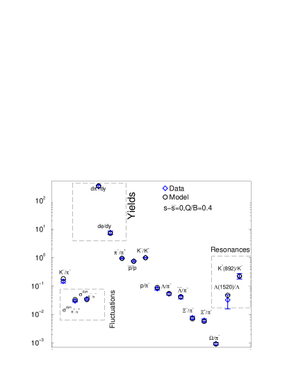
We have performed a fit incorporating all ratios from barannikova , with the exception of the $\Delta^{++}/p$, which the STAR collaboration has taken back, and the $\overline{\Omega}/\Omega$, measured by STAR to be above unity (The latter measurement is a priori incompatible with statistical production liu ). In addition, we have included the preliminary value for the $K/\pi$ event-by-event fluctuation measured by STAR supriya , as well as the published yield for $\phi$ starphi200 and $\pi^{-}$ starpi200 .

Our fit parameters include the normalization (hopefully related to the system “volume” at chemical freeze-out), temperature, $\lambda_{q,s,I_{3}}$ and $\gamma_{q,s}$. We also require, by implementing them as data-points, strangeness, charge and baryon number conservation
($\left\langle s-\overline{s}\right\rangle=0\phantom{AA}\left\langle Q\right\rangle/\left\langle B\right\rangle=(\left\langle Q\right\rangle/\left\langle B\right\rangle)_{Au}=0.4.)$.

The result is shown in Fig. 1. The fit gives an adequate description of all particle yields, including the resonance $K^{*}/K^{-}$ and $\Lambda(1520)/\Lambda$. It can also, adequately describe the event-by-event fluctuations of of $K^{+}/\pi^{+}$ or $K^{-}/\pi^{-}$, but not the difference between them. Describing the difference within the SHM is impossible without introducing a sizable isospin fugacity $\lambda_{I3}\sim 0.96$ which is in turn excluded by ratios such as $\pi^{+}/\pi^{-}$ and $Q/B$. We wait for published results, and systematic error computation before studying this discrepancy further.

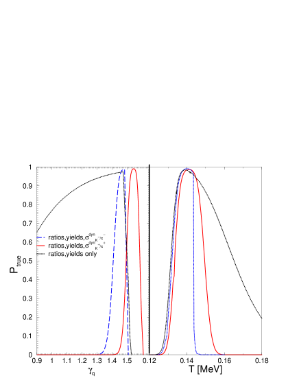
Fig. 2 shows that the correlation between $T$ and $\gamma_{q}$ disappears when fluctuations are taken into account, and that the fit tightly constrains $\gamma_{q}$ well above the equilibrium value, forcing temperature to be about 140 MeV, in good agreement of the prediction of the supercooled hadronization scenario. In accordance with this scenario, our model can describe both the $K/\pi$ fluctuation and the directly observed $K^{*}/K^{-}$ value with the same statistical parameters, as is expected for a system where hadronic reinteraction (the phase between chemical freeze-out and thermal freeze-out) is negligible.

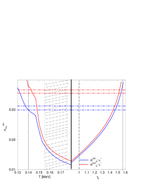
Fig. 3 confirms that fluctuations are indeed responsible for the tight constraining of $T$ and $\gamma_{q}$. The best fit at light quark equilibrium misses $\sigma_{K/\pi}^{dyn}$ by several standard deviations. Introducing exact conservation for strangeness within the observed window would increase the discrepancy by reducing $\sigma_{K}$ nogc2 . It is only through $\gamma_{q}>1$ that $\sigma_{K/\pi}^{dyn}$ increases until it becomes compatible with the experimental value.

Figure 3: Sensitivity of the $K/\pi$ fluctuation $(\sigma_{K/\pi}^{dyn})$ to $\gamma_{q}$ and temperature for the fit in Fig. 1. At each point in the abscissa, a fit is performed (only yield data-points used) varying all fit parameters except the one on the abscissa. $\sigma_{K/\pi}^{dyn}$ is calculated using the best fit parameters. dot-dashed lines refer to the experimental limits supriya for the $\sigma_{K^{+}/\pi^{+}}$ (blue) and $\sigma_{K^{-}/\pi^{-}}$ (red). Dotted vertical lines give published non-equilibrium best fit parameters gammaq_energy , while the long-dashed line and shaded area gives published equilibrium best fit barannikova ; bdm ; gammaq_energy .

In conclusion, we have used preliminary experimental data to show that, at 200 GeV, the equilibrium model is unable to describe both yields and fluctuations within the same statistical parameters. The non-equilibrium model, in contrast, succeeds in describing almost all of the yields and fluctuations measured so far at RHIC, with the parameters expected from a scenario where non-equilibrium arises through a phase transition from a high entropy state, with super-cooling and oversaturation of phase space. We await more published data to determine weather the non-equilibrium model is really capable of accounting for both yields and fluctuations in all light and strange hadrons produced in heavy ion collisions.

Work supported in part by grants from the U.S. Department of Energy (J.R. by DE-FG02-04ER41318) the Natural Sciences and Engineering research council of Canada, the Fonds Nature et Technologies of Quebec. G. T. thanks the Tomlinson foundation for support, and the QM2005 organizers for financial support during the conference. S.J. thanks RIKEN BNL Center and U.S. Department of Energy [DE-AC02-98CH10886] for providing facilities essential for the completion of this work.

References

- (1) E. Fermi, Prog. Theor. Phys. 5, 570 (1950).
- (2) I. Pomeranchuk, Proc. USSR Academy of Sciences (in Russian) 43, 889 (1951).
- (3) L. D. Landau, Izv. Akad. Nauk Ser. Fiz. 17 (1953) 51.
- (4) R. Hagedorn, Suppl. Nuovo Cimento 2, 147 (1965).
- (5) S. Jeon, V. Koch, K. Redlich and X. N. Wang, Nucl. Phys. A 697, 546 (2002)
- (6) S. Jeon and V. Koch, Phys. Rev. Lett. 83, 5435 (1999)
- (7) S. Jeon and V. Koch, Phys. Rev. Lett. 85, 2076 (2000)
- (8) C. Pruneau, S. Gavin and S. Voloshin, Phys. Rev. C 66, 044904 (2002) [arXiv:nucl-ex/0204011].
- (9) J. Adams et al. [STAR Collaboration], Phys. Rev. C 68, 044905 (2003)
- (10) K. Adcox et al. [PHENIX Collaboration], Phys. Rev. Lett. 89, 082301 (2002)
- (11) V. V. Begun, M. Gazdzicki, M. I. Gorenstein and O. S. Zozulya, Phys. Rev. C 70, 034901 (2004).
- (12) G. Torrieri, et al., Comm. in Computer physics in press arXiv:nucl-th/0404083
- (13) J. Cleymans, K. Redlich, Phys. Rev. C 60, 054908 (1999).
- (14) G. Torrieri, S. Jeon, J. Rafelski Submitted to PRL [arXiv:nucl-th/0503026].
- (15) J. Letessier and J. Rafelski, Cambridge Monogr. Part. Phys. Nucl. Phys. Cosmol. 18, 1 (2002),
-
(16)
See most advanced physical chemistry textbooks, or
http://www2.mcdaniel.edu/Chemistry/ch307.notes/
Chemical20Equilibrium.html - (17) J. Rafelski and J. Letessier, Phys. Rev. Lett. 85, 4695 (2000).
- (18) T. Csorgo and L. Csernai, arXiv:hep-ph/9312330
- (19) J. Letessier and J. Rafelski, Int. J. Mod. Phys. E 9, 107, (2000), and references therein.
- (20) J. Rafelski, J. Letessier, J. Phys. G 30, S1 (2004).
- (21) J. Letessier and J. Rafelski, arXiv:nucl-th/0504028.
- (22) D. Flierl et al. [NA49 Collaboration], arXiv:nucl-ex/0410041.
- (23) J. Rafelski, J. Letessier and G. Torrieri, Phys. Rev. C 72, 024905 (2005) [arXiv:nucl-th/0412072].
- (24) O. Barannikova [STAR Collaboration], arXiv:nucl-ex/0403014 and references therein.
- (25) P. Braun-Munzinger, D. Magestro, K. Redlich and J. Stachel, Phys. Lett. B 518, 41 (2001).
- (26) G. Torrieri and J. Rafelski, arXiv:hep-ph/0409160.
- (27) S. Das [STAR Collaboration], arXiv:nucl-ex/0503023.
- (28) C. Pruneau, S. Gavin and S. Voloshin, Phys. Rev. C 66, 044904 (2002) [arXiv:nucl-ex/0204011].
- (29) M. Bleicher et al., Phys. Rev. Lett. 88, 202501 (2002) [arXiv:hep-ph/0111187].
- (30) J. Adams et al. [STAR Collaboration], Phy. Lett. B in press, [arXiv:nucl-ex/0406003].
- (31) J. Adams et al. [STAR Collaboration], Phys. Rev. Lett. 92, 112301 (2004) [arXiv:nucl-ex/0310004].