Particle spectra and hydro-inspired models

Abstract

Several popular parameterizations of the freeze-out conditions in ultra-relativistic heavy-ion collisions are shortly reviewed. The common features of the models, responsible for the successful description of hadronic observables, are outlined.

1 INTRODUCTION

In this talk I present several models which turned out to be quite successful in reproducing the experimentally measured hadron spectra in nucleus-nucleus collisions. The discussed models use concepts borrowed from relativistic hydrodynamics but they do not include the complete time evolution of the system. For this reason, they may be called hydro-inspired (freeze-out) models. The measured particle spectra reflect properties of matter at the stage when particles stop to interact. This moment is called the kinetic (thermal) freeze-out. Hydro-inspired models help us to verify the idea that matter, just before the kinetic freeze-out, is locally thermalized and exhibits collective behavior, such as the transverse and longitudinal expansion. If this is really the case, i.e., if the hydro-inspired models describe the data well, we may infer the thermodynamic properties of matter at freeze-out, such as the values of the temperature and flow, and request that the advanced hydrodynamic models reproduce this configuration.

In my opinion, the real aim of the freeze-out models is to form a simple link between sophisticated hydrodynamic calculations [1, 2, 3, 4, 5, 6] describing the full time evolution of matter (with the inclusion of the phase transition) and the rich bulk of the experimental data describing soft phenomena. This is an appealing idea, however, one encounters several problems on the way to achieve this task, since certain features of the hydrodynamic models and the freeze-out models are quite different. For example, at the first sight one can realize that typical shapes of the freeze-out hypersurfaces used in the advanced hydro calculations and in the freeze-out models are quite different. Clearly, further work is necessary to make the connection between the hydro calculations and the freeze-out models more consistent.

In any case, an attractive feature of the hydro-inspired models is that they are very effective parameterizations of the final state, that use few parameters possessing clear physical interpretation. As long as we do not all have hydrodynamic codes that we are able to run on our PCs, the freeze-out models form a very convenient and easy accessible tool to interpret the data. In this talk I intend to review several models which give consistent description of many observables (not only of the particle spectra). Their list includes: different versions of the blast-wave model [7, 8], the Buda-Lund model [9, 10, 11], the Seattle model [12, 13], the Durham model [14, 15], the Cracow single-freeze-out model [16, 17, 18], and THERMINATOR [19].

Below, I will refer only to the Au+Au collisions studied at the top RHIC energies; I want to show how different models describe the same set of data rather than to show how one model is able to describe different physical situations. Examples of the application of the thermal approach to calculate the spectra at lower energies may be found in Refs. [20, 21].

2 COOPER-FRYE FORMULA AND EMISSION FUNCTION

Before going into the discussion of the blast-wave model, I would like to make a few remarks about the Cooper-Frye formula [22]. It is frequently used in the hydrodynamic calculations to obtain the momentum distribution of the emitted particles. In this talk, the Cooper-Frye formula will serve us as a reference point for the characteristics of different freeze-out models. Its standard form is

$$E_{p}{dN\over d^{3}p}=\int\,p^{\mu}d\Sigma_{\mu}(x)\,f_{\rm eq}\left(p\cdot u(x)\right),$$ (1)

where $E_{p}=\sqrt{m^{2}+{\bf p}^{2}}$ is the energy of a particle, $d\Sigma^{\mu}(x)$ a three-dimensional element of the freeze-out hypersurface, $u^{\mu}(x)$ is the hydrodynamic flow, and $f_{\rm eq}$ is the equilibrium distribution function. In the general case, the hypersurface includes the time-like (defined here by the condition: $d\Sigma^{\mu}d\Sigma_{\mu}=(d\Sigma_{0})^{2}-(d\Sigma_{1})^{2}-(d\Sigma_{2})^{2}-(d\Sigma_{3})^{2}>0$) and space-like ($d\Sigma^{\mu}d\Sigma_{\mu}<0$) parts. The advanced hydrodynamic calculations include both parts, while hydro-inspired models include typically only the time-like parts. The success of the hydro-inspired models may indicate that the contributions from the space-like parts are negligible. On the other hand, detailed microscopic studies show that the contributions from those parts are substantial and difficult to include in the consistent way, unless one uses the approach based on the kinetic theory [23, 24, 25, 26, 27, 28, 29, 30, 31, 32, 33].

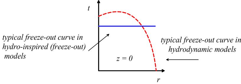
Figure 1: Freeze-out curves in the Minkowski space, i.e., projections of the freeze-out hypersurfaces on the plane $z=0$ for cylindrically symmetric systems, in the advanced hydro calculations (dashed line) and in the freeze-out models (solid line).

The Cooper-Frye formula may be rewritten in such a way that the distribution of the particles in the momentum space is given as the space-time integral over the so-called emission or source function

$$E_{p}{dN\over d^{3}p}=\int d^{4}x\int\,p^{\mu}d\Sigma_{\mu}(x^{\prime})\delta^{4}(x^{\prime}-x)\,f_{\rm eq}\left(p\cdot u(x^{\prime})\right)\equiv\int d^{4}x\,S(x,p).$$ (2)

The emission function defines the space-time distribution of the points from which the observed hadrons are emitted. Very often Eq. (2) is used with $S(x,p)$ modeled without any reference to the Cooper-Frye formula. Such a procedure lays emphasis on the fact that the hydro-inspired models should aim mainly at the reconstruction of the realistic emission function.

3 BLAST-WAVE MODELS

Different versions of the blast-wave model originate from the paper by Siemens and Rasmussen [34], where a relativistic formula for the particle distribution corresponding to a thermalized and radially expanding system was first given. More recent applications use the same concepts but different geometries of the expansion, more suitable for the description of the ultra-relativistic heavy-ion collisions, are considered [35].

3.1 Cylindrically symmetric systems

For boost-invariant and cylindrically symmetric systems, the Cooper-Frye formula (1) leads to the very popular model of Schnedermann, Sollfrank and Heinz [7]. For constant transverse flow, $v_{T}$ = tanh$\rho$ = const, one obtains the rapidity and transverse-momentum distribution of the emitted particles in the form

$${dN\over dyd^{2}p_{T}} = {e^{\beta\mu}\over 2\pi^{2}}m_{T}K_{1}\left[\beta m_{T}\hbox{cosh}(\rho)\right]I_{0}\left[\beta p_{T}\hbox{sinh}(\rho)\right]\int\limits_{0}^{1}d\zeta\,\,r(\zeta)t(\zeta){dr\over d\zeta}$$ (3)

$$-{e^{\beta\mu}\over 2\pi^{2}}p_{T}K_{0}\left[\beta m_{T}\hbox{cosh}(\rho)\right]I_{1}\left[\beta p_{T}\hbox{sinh}(\rho)\right]\int\limits_{0}^{1}d\zeta\,\,r(\zeta)t(\zeta){dt\over d\zeta},$$

where $m_{T}=\sqrt{m^{2}+p_{T}^{2}}$ is the transverse mass, $\beta=1/T$ is the inverse temperature, $\mu$ is the chemical potential, $\rho$ is the transverse rapidity, $t$ and $r=\sqrt{r_{x}^{2}+r_{y}^{2}}$ are the coordinates of the freeze-out hypersurface at $z=0$, while $K_{0,1}$ and $I_{0,1}$ are the modified Bessel functions. The integrals on the right-hand-side of Eq. (3) involve the parameterizations of the freeze-out position coordinates and times in terms of the parameter $\zeta$. In practical applications, the second line on the right-hand-side of Eq. (3) is very often neglected, which means that the variations of the emission times are ignored. This procedure implicitly denotes that the particle emission takes place at a constant laboratory time (at $z=0$), see Fig. 1.

An example of the procedure outlined above is the blast-wave fit performed recently by the BRAHMS Collaboration [36]. The optimal value of the temperature obtained from the fit to the Au+Au data ($\sqrt{s_{NN}}$ = 200 GeV, midrapidity region, centrality class 0-10%) is 110 MeV, while the average transverse flow velocity equals 0.65 $c$. In this, and other similar cases, we have to be aware that a theoretical boost-invariant model has been applied to the system which is not boost-invariant as a whole. In my opinion, such procedure is justified only at the top RHIC energies in the midrapidity region where the rapidity distribution may be regarded as flat within 1 or at most 2 units of rapidity.

3.2 Cylindrically non-symmetric systems

For boost-invariant and cylindrically non-symmetric systems one may use the parameterization of the emission function introduced by Retière and Lisa [8]. It takes into account the possible ellipsoidal shape of the system created in non central collisions. The emission function proposed in [8] may be obtained from the Cooper-Frye formula if the constant evolution time, $\tau=\tau_{0}$ = const, is replaced by a gaussian distribution

$$S(x,p)=Z\,m_{T}\cosh(\eta-y)\,\Omega(r,\phi_{s})\,e^{\frac{-(\tau-\tau_{0})^{2}}{2\Delta\tau^{2}}}\,\frac{1}{e^{p\cdot u/T}\pm 1}.$$ (4)

Here $Z$ is an arbitrary normalization constant, $\eta=1/2\ln\,(t+z)/(t-z)$ is the spacetime rapidity, $\tan\phi_{s}=r_{y}/r_{x}$, $\Delta\tau$ is the emission time, and $\Omega$ describes the spatial distribution of matter in the transverse plane

$$\Omega(r,\phi_{s})=\Omega(\tilde{r})=\frac{1}{1+e^{(\tilde{r}-1)/a_{s}}},\hskip 28.45274pt\tilde{r}(r,\phi_{s})\equiv\sqrt{\frac{(r\cos(\phi_{s}))^{2}}{R_{x}^{2}}+\frac{(r\sin(\phi_{s}))^{2}}{R_{y}^{2}}}.$$ (5)

The parameter $a_{s}$ describes the surface diffuseness of the source. In the limit $a_{s}\to 0$, the matter in the transverse plane is confined in an ellipse defined by the parameters $R_{x}$ and $R_{y}$. The explicit form of the flow field $u^{\mu}$ (and of the expression $p\cdot u$) is given in Ref. [8], here we only note that the expansion velocity in the transverse plane is perpendicular to the elliptical shell confining the matter.

The optimal values of the temperature obtained by Retière and Lisa in their analysis of three different centrality classes (0-5%, 15-30%, 60-92%, the Au+Au collisions at the beam energy of $\sqrt{s_{NN}}$ = 130 GeV, combined PHENIX and STAR data [37, 38]) are: 107, 106, and 100 MeV, respectively. The corresponding values of the transverse flow are: 0.52 $c$, 0.50 $c$, and 0.47 $c$.

3.3 Summary on the blast-wave models

When applied to the Au+Au collisions at the top RHIC energies, the blast-wave models give good description of the $p_{T}$-spectra, the elliptic flow, and the HBT radii at midrapidity. An interesting feature of the Retière-Lisa model is that it includes, as the special case, the situation where the in-plane flow is not stronger than the out-of-plane flow, but the correct sign and magnitude of the coefficient $v_{2}$ is reproduced. This feature is realized by the geometry of the model which implies in this case that more matter flows in the reaction plane than out of the reaction plane.

The blast-wave fits to the data indicate short evolution times, $\tau\leq 10$ fm, and very short emission times, $\Delta\tau\leq 1$ fm. The typical value of the temperature is about 100 MeV. The blast-wave models do not predict the absolute normalization of the spectra, hence an extra parameter is required to normalize each considered spectrum. In addition, many of the applications of the blast-wave model do not include the effects of the decays of resonances.

4 BUDA-LUND MODEL

The standard version of the Buda-Lund model was formulated to describe cylindrically symmetric systems with no constraint of the boost-invariance [9, 10]. Later the model was extended to describe ellipsoidally symmetric systems [11]. The standard emission function of the model has the form

$$S(x,p)={g\over(2\pi)^{3}}\,\,{m_{T}\cosh(\eta-y)\over\exp\left({u^{\mu}(x)p_{\mu}\over T(x)}-{\mu(x)\over T(x)}\right)\pm 1}\,\frac{1}{(2\pi\Delta\tau^{2})^{1/2}}\exp\left[-\frac{(\tau-\tau_{0})^{2}}{2\Delta\tau^{2}}\right],$$ (6)

where the temperature and chemical potential depend on the position coordinates

$${\mu(x)\over T(x)}={\mu_{0}\over T_{0}}-{r^{2}\over 2R_{G}^{2}}-{\eta^{2}\over 2\Delta\eta^{2}},$$ (7)

$${1\over T(x)}={1\over T_{0}}\,\,\left(1+{T_{0}-T_{s}\over T_{s}}\,{r^{2}\over 2R_{G}^{2}}\right)\,\left(1+{T_{0}-T_{\rm e}\over T_{\rm e}}\,{(\tau-\tau_{0})^{2}\over 2\Delta\tau^{2}}\right).$$ (8)

In Eq. (8), the quantity $T_{0}$ is the temperature in the center at the mean freeze-out time, $T_{\rm s}$ is the temperature on the surface at the mean freeze-out time, and $T_{\rm e}$ is the temperature in the center at the end of particle emission. The flow pattern assumed in the Buda-Lund model has a Hubble-like structure, with the velocity of the fluid element proportional to its distance from the center. Such patterns appear in the analytic [39] and numerical [40] solutions of the equations of the relativistic hydrodynamics. For physical interpretation of other model parameters we refer to the original papers [9, 10].

The Buda-Lund model gives a very good description of the $p_{T}$-spectra, $v_{2}$ and HBT radii in the full rapidity range. The fits to the experimental data indicate small values of the evolution and emission times which are compatible with those obtained from the blast-wave analysis (for Au+Au at $\sqrt{s_{NN}}$ = 200 GeV the optimal Buda-Lund fit yields: $T_{0}$ = 196 MeV, $T_{\rm e}$ = 117 MeV, $T_{s}$ = 89.7 MeV, $R_{G}$ = 13.5 fm, $R_{s}$ = 12.4 fm, $\tau_{0}=$ 5.8 fm, $\Delta\tau=$ 0.9 fm, and $\Delta\eta$ = 3.1). The effects of the decays of resonances are not included explicitly and the information about the normalization of the spectra is derived from the HBT data. The Buda-Lund fits indicate a freeze-out temperature distribution, with an average freeze-out temperature of 100 - 120 MeV. However, about 1/8th of the particles is found to be emitted from a very hot center with $T\sim$ 200 MeV. A comparison of this result with the lattice QCD results for the critical temperature was considered as an indication of quark deconfinement in Ref. [41].

5 SEATTLE MODEL

The Seattle model formulated in Refs. [12, 13] describes cylindrically symmetric systems. No assumption about the boost-invariance is made. The main characteristic feature of the model is inclusion of the effects of the final-state interaction of the outgoing pions. Such effects are taken into account by the use of the distorted wave functions $\Psi_{{\bf p}}^{(-)}(x)$. The formalism, following Ref. [42], is based on the generalized emission function, which may be used to get the one-particle and two-particle distributions in the momentum space

$$S(x,p,q)=\int d^{4}K^{\prime}S_{0}(x,K^{\prime})\int{d^{4}x^{\prime}\over(2\pi)^{4}}\;e^{-iK^{\prime}\cdot x^{\prime}}\Psi_{{\bf p}_{1}}^{(-)}(x+x^{\prime}/2)\Psi_{{\bf p}_{2}}^{(-)*}(x-x^{\prime}/2),$$ (9)

$$p=(p_{1}+p_{2})/2,\quad q=p_{1}-p_{2}.$$ (10)

The quantities $p_{1}$ and $p_{2}$ are the pion four-momenta. In the special case, where the distorted wave functions are replaced by the plane waves, the standard formulation is recovered with the emission function reduced to $S_{0}$,

$$\Psi_{{\bf p}}^{(-)}(x)\to e^{ip\cdot x},\quad S(x,p,q)\to S_{0}(x,p)e^{iq\cdot x},\quad S(x,p,0)\to S_{0}(x,p).$$ (11)

The function $S_{0}$ resembles the parameterization used in the Buda-Lund model, however, in this case the thermodynamic parameters are constant,

$$S_{0}(x,p)=\frac{m_{T}\cosh\eta}{\sqrt{2\pi(\Delta\tau)^{2}}}\exp\left[-{(\tau-\tau_{0})^{2}\over 2\Delta\tau^{2}}-{\eta^{2}\over 2\Delta\eta^{2}}\right]{\Omega(r)\over(2\pi)^{3}}{1\over\exp({p\cdot u-\mu_{\pi}\over T})-1}.$$ (12)

The distribution of matter is characterized by the function

$$\Omega(r)={1\over\left[\exp\left({r-R_{WS}\over a_{WS}}\right)+1\right]^{2}},\quad r=\sqrt{r_{x}^{2}+r_{y}^{2}}.$$ (13)

The optimal values of the parameters obtained from the fit to the STAR data [43] describing the Au+Au collisions at $\sqrt{s_{NN}}=200$ GeV are the following [13]: $T$ = 215 MeV, $\mu_{\pi}$ = 123 MeV, $\tau_{0}$ = 8 fm, $\Delta\tau$ = 2.7 fm, $R_{WS}$ = 12 fm, $a_{WS}$ = 0.8 fm, $\Delta\eta$ = 1, $\eta_{f}$ = 1.5, $w_{0}$ = 0.142$\pm$0.046 fm^-2, and $w_{2}$ = 0.582 $\pm$ 0.014 + $i$(0.123$\pm$0.002). The parameter $\eta_{f}$ defines the magnitude of the transverse flow [12], whereas the parameters $w_{0}$ and $w_{2}$ define the optical potential which modifies the outgoing pion wave functions. The strength of the attraction inside the medium is greater than $m^{2}_{\pi}$, hence a pion behaves to large extent as a massless particle. This behavior may be related to the phenomena discussed in Refs. [44, 45].

The Seattle model describes successfully the pion transverse-momentum spectra and the HBT radii in the region $p_{T}>100$ MeV. On the other hand, the model predicts non-monotonic structures in the transverse-momentum region below 70 MeV. Such predictions were confronted with the PHOBOS data in Ref. [46] and certain discrepancies between the data and the model were found. Very likely the non-monotonic structures are due to the sudden change of the optical potential in the transverse direction and a better agreement with the data may be achieved by the modification of this dependence.

6 DURHAM MODEL

The Durham model, proposed by Renk in Refs. [14, 15], is based on the parameterization of the hydrodynamic expansion in the proper-time interval $\tau_{0}\leq\tau\leq\tau_{f}$. The pressure profiles determine the evolution of the boundaries of the system, then the boundaries determine the evolution of the entropy density. In the next step, the equation of state is used to calculate the pressure. The iterative procedure ensures that this approach is self-consistent, i.e., the pressure profiles which determine the evolution of the system agree with the pressure obtained from the equation of state. The freeze-out happens at a fixed temperature $T_{f}$ and the Cooper-Frye formula is used to calculate the spectra. The optimal parameters obtained from the fit to the PHENIX data [47, 48] include: $\tau_{0}$ = 1 fm, $\tau_{f}$ = 19 fm, $T_{f}$ = 110 MeV. The Durham model describes nicely the $p_{T}$-spectra and HBT radii. No resonance decays are included in the calculation of the spectra. In my opinion, a direct comparison with the real hydrodynamic calculations will strengthen the importance of this model, if the validity of the proposed parameterization is confirmed.

7 CRACOW SINGLE-FREEZE-OUT MODEL

The standard version of this model [16] describes boost-invariant and cylindrically symmetric systems. The model is based on the extreme assumption that the chemical and kinetic freeze-outs coincide. The thermodynamic parameters of the model are obtained from the analysis of the ratios of hadron abundances [49]. In this respect the Cracow model is closely related to different statistical models developed recently by many groups [50, 51, 52, 53, 54, 55]. An important feature of the model is that a complete set of hadronic resonances is included in the calculation of various physical observables. The resonances are included by the use of the emission function that corresponds to the Cooper-Frye formula convoluted with the momentum splitting functions $B$ and the space-time displacement functions $\delta$,

$$S\left(x_{1},p_{1}\right)=E_{1}{dN_{1}\over d^{3}p_{1}d^{4}x_{1}}=$$

$$\int\frac{d^{3}p_{2}}{E_{p_{2}}}B\left(p_{2},p_{1}\right)\int d\tau_{2}\Gamma_{2}e^{-\Gamma_{2}\tau_{2}}\int d^{4}x_{2}\delta^{\left(4\right)}\left(x_{2}+\frac{p_{2}\tau_{2}}{m_{2}}-x_{1}\right)...$$

$$\hskip 14.22636pt\times\int d\Sigma_{\mu}\left(x_{N}\right)\,p_{N}^{\mu}\,\,\delta^{\left(4\right)}\left(x_{N}+\frac{p_{N}\,\tau_{N}}{m_{N}}-x_{N-1}\right)f_{N}\left[p_{N}\cdot u\left(x_{N}\right)\right]$$ (14)

Here the indices $1,...,N$ denote particles in a cascade of decaying resonances ($N$ refers to the resonance decaying on the freeze-out hypersurface, while $1$ refers to the final observed particle, e.g., a pion, other symbols are defined in [16, 17, 18]). The freeze-out hypersurface is defined by the conditions:

$$\tau_{\rm inv}=\sqrt{t^{2}-r^{2}_{x}-r^{2}_{y}-r^{2}_{z}}={\rm const},\quad r=\sqrt{r_{x}^{2}+r_{y}^{2}}<r_{\rm max}$$ (15)

$$u^{\mu}=\frac{x^{\mu}}{\tau_{\rm inv}}=\frac{t}{\tau_{\rm inv}}\left(1,\frac{r_{x}}{t},\frac{r_{y}}{t},\frac{r_{z}}{t}\right),\quad d\Sigma^{\mu}=u^{\mu}\,\tau_{\rm inv}^{3}\,{\rm sinh}(\rho){\rm cosh}(\rho)\,d\rho d\eta d\phi.$$ (16)

The standard version of the model uses only 4 parameters: temperature ($T$), baryon chemical potential ($\mu_{B}$), $\tau_{\rm inv}$, and $r_{\rm max}$. The values of the temperature and baryon chemical potential, obtained from the analysis of the ratios of hadron abundances, are independent of centrality. For the top RHIC energies one finds $T=165.5$ MeV and $\mu_{B}=28.5$ MeV. The expansion parameters $\tau_{\rm inv}$ and $r_{\rm max}$ are determined by the fits to the $p_{T}$-spectra, and their values depend on centrality [56].

The Cracow model gives a good description of the ratios of hadronic observables, $p_{T}$-spectra, the HBT radii $R_{\rm side}$ and $R_{\rm out}$. It also gives satisfactory description of the balance functions [57] and of the invariant masses of the pion pairs [58]. Generalizations of the model describing systems without cylindrical symmetry [59] or boost-invariance [35] were proposed to account for the observed values of the coefficient $v_{2}$ and the $p_{T}$-spectra at finite values of the rapidity as measured by BRAHMS [60].

8 THERMINATOR, SHARE, THERMUS

THERMINATOR [19] is the Monte-Carlo version of the Cracow and blast-wave models (the blast-wave model has been extended in this case to include the complete set of hadronic resonances). The program uses the same input from the Particle Data Tables [61] as SHARE [62]. With the physical input of the thermodynamic and expansion parameters, THERMINATOR delivers the full space-time information about cascades of decaying resonances. The values of the thermodynamic parameters may be taken from SHARE or from other programs used to study the ratios of hadronic abundances, for example from THERMUS [63]. The information about the space-time positions of the produced hadrons may be used to study different types of correlations. Moreover, the Monte-Carlo approach facilitates the inclusion of the experimental cuts and acceptance.

9 HUMANIC’S RESCATTERING MODEL

In the end of this talk I would like to note that simple transport models may play a similar role as hydro-inspired models. An example of such approach is Humanic’s model [64]. This model is a Monte-Carlo simulation of the evolution of purely hadronic system. The initialization stage may be considered as equivalent to the hadronization process. The transverse geometry is determined by the overlapping region of the two colliding nuclei, while the initial $p_{T}$- and $y$-distributions are assumed to have the following shape

$${1\over m_{T}}{dN\over dm_{T}}=C{m_{T}\over\exp(m_{T}/T)\pm 1},\quad{dN\over dy}=De^{-{(y-y_{0})^{2}\over 2\sigma_{y}^{2}}},$$ (17)

with the optimal parameters: $T$ = 300 MeV and $\sigma_{y}$ = 2.4. The longitudinal positions and times of the initialized hadrons are: $z_{\rm had}=\tau_{\rm had}\,\hbox{sinh}y$ and $t_{\rm had}=\tau_{\rm had}\,\hbox{cosh}y$, where $\tau_{\rm had}$ is the initial (proper) time, with the standard value of 1 fm.

The subsequent evolution of the system includes binary collisions of: $\pi$, $K$, $N$, $\Delta$, $\Lambda$, $\rho$, $\omega$, $\eta$, $\eta^{\prime}$, $\phi$ and $K^{*}$. The freeze-out happens (dynamically) at about 30 fm (Au+Au, 130 GeV). The model gives successful description of the slope parameters, $v_{2}(m,p_{T},\eta)$, and the $p_{T}$ and centrality dependence of the HBT radii. The results are sensitive to $\tau_{\rm had}$; larger values of $\tau_{\rm had}$ imply fewer collisions and the rescattering-generated flow is reduced.

10 CONCLUSIONS

A common feature of the hydro-inspired models is the short evolution time, $\tau_{0}<$ 10 fm, and even shorter emission time $\Delta\tau<<\tau_{0}$. Another common feature is a large value of the transverse flow, $\langle v_{t}\rangle\sim 0.5$ c. Altogether, these observations indicate an explosive scenario for the Au+Au collisions observed at the top RHIC energies.

Models which do not include resonances or pion final-state interactions, yield rather low values of the freeze-out temperature, $T\sim 100$ MeV. We know, however, that the effects of the resonance decays must be important, since large abundances of certain resonances were observed [65, 66]. In this situation, I think that the hydro-inspired models should enter a new stage where the effects of both the transverse flow and the resonance decays are commonly taken into account. Another development of the hydro-inspired models should include the emission from the space-like parts. An example of such approach is a recent paper by the Kiev-Nantes group [67].

References

- [1] D. Teaney, J. Lauret and E.V. Shuryak, (2001), nucl-th/0110037.
- [2] P. Huovinen, Acta Phys. Polon. B33 (2002) 1635, nucl-th/0204029.
- [3] P.F. Kolb and R. Rapp, Phys. Rev. C67 (2003) 044903, hep-ph/0210222.
- [4] P.F. Kolb and U. Heinz, (2003), nucl-th/0305084.
- [5] T. Hirano, J. Phys. G30 (2004) S845, nucl-th/0403042.
- [6] J. Socolowski, O. et al., Phys. Rev. Lett. 93 (2004) 182301, hep-ph/0405181.
- [7] E. Schnedermann, J. Sollfrank and U.W. Heinz, Phys. Rev. C48 (1993) 2462, nucl-th/9307020.
- [8] F. Retière and M.A. Lisa, Phys. Rev. C70 (2004) 044907, nucl-th/0312024.
- [9] T. Csörgő and B. Lörstad, Phys. Rev. C54 (1996) 1390, hep-ph/9509213.
- [10] T. Csörgő, Heavy Ion Phys. 15 (2002) 1, hep-ph/0001233.
- [11] M. Csanád, T. Csörgő and B. Lörstad, Nucl. Phys. A742 (2004) 80, nucl-th/0310040.
- [12] J.G. Cramer et al., Phys. Rev. Lett. 94 (2005) 102302, nucl-th/0411031.
- [13] G.A. Miller and J.G. Cramer, (2005), nucl-th/0507004.
- [14] T. Renk, Phys. Rev. C70 (2004) 021903, hep-ph/0404140.
- [15] T. Renk, J. Phys. G30 (2004) 1495, hep-ph/0403239.
- [16] W. Broniowski and W. Florkowski, Phys. Rev. Lett. 87 (2001) 272302, nucl-th/0106050.
- [17] W. Broniowski and W. Florkowski, Phys. Rev. C65 (2002) 064905, nucl-th/0112043.
- [18] W. Broniowski, A. Baran and W. Florkowski, Acta Phys. Polon. B33 (2002) 4235, hep-ph/0209286.
- [19] A. Kisiel et al., (2005), nucl-th/0504047.
- [20] G. Torrieri and J. Rafelski, New J. Phys. 3 (2001) 12, hep-ph/0012102.
- [21] J. Letessier et al., J. Phys. G27 (2001) 427, nucl-th/0011048.
- [22] F. Cooper and G. Frye, Phys. Rev. D10 (1974) 186.
- [23] K.A. Bugaev, Nucl. Phys. A606 (1996) 559.
- [24] C. Anderlik et al., Phys. Rev. C59 (1999) 3309, nucl-th/9806004.
- [25] V.K. Magas et al., Nucl. Phys. A661 (1999) 596, nucl-th/0001049.
- [26] Y.M. Sinyukov, S.V. Akkelin and Y. Hama, Phys. Rev. Lett. 89 (2002) 052301, nucl-th/0201015.
- [27] K.A. Bugaev, Phys. Rev. Lett. 90 (2003) 252301, nucl-th/0210087.
- [28] V.K. Magas et al., Eur. Phys. J. C30 (2003) 255, nucl-th/0307017.
- [29] K.A. Bugaev, Phys. Rev. C70 (2004) 034903, nucl-th/0401060.
- [30] F. Grassi, Braz. J. Phys. 35 (2005) 52, nucl-th/0412082.
- [31] E. Molnár et al., (2005), nucl-th/0503048.
- [32] E. Molnár et al., (2005), nucl-th/0503047.
- [33] K. Tamosiunas et al., J. Phys. G31 (2005) S1001.
- [34] P.J. Siemens and J.O. Rasmussen, Phys. Rev. Lett. 42 (1979) 880.
- [35] W. Florkowski and W. Broniowski, Acta Phys. Polon. B35 (2004) 2895, nucl-th/0410081.
- [36] BRAHMS, I. Arsene et al., Phys. Rev. C72 (2005) 014908, nucl-ex/0503010.
- [37] PHENIX, K. Adcox et al., Phys. Rev. Lett. 88 (2002) 242301, nucl-ex/0112006.
- [38] STAR, C. Adler et al., Phys. Rev. Lett. 89 (2002) 092301, nucl-ex/0203016.
- [39] T. Csörgő et al., Phys. Lett. B565 (2003) 107, nucl-th/0305059.
- [40] M. Chojnacki, W. Florkowski and T. Csörgő, (2004), nucl-th/0410036.
- [41] M. Csanád et al., J. Phys. G30 (2004) S1079, nucl-th/0403074.
- [42] M. Gyulassy, S.K. Kauffmann and L.W. Wilson, Phys. Rev. C20 (1979) 2267.
- [43] STAR, J. Adams et al., Phys. Rev. Lett. 92 (2004) 112301, nucl-ex/0310004.
- [44] T.D. Cohen and W. Broniowski, Phys. Lett. B342 (1995) 25, hep-ph/9407354.
- [45] D.T. Son and M.A. Stephanov, Phys. Rev. Lett. 88 (2002) 202302, hep-ph/0111100.
- [46] PHOBOS, B.B. Back et al., (2005), nucl-ex/0506008.
- [47] PHENIX, S.S. Adler et al., Phys. Rev. C69 (2004) 034909, nucl-ex/0307022.
- [48] PHENIX, S.S. Adler et al., Phys. Rev. Lett. 93 (2004) 152302, nucl-ex/0401003.
- [49] W. Florkowski, W. Broniowski and M. Michalec, Acta Phys. Polon. B33 (2002) 761, nucl-th/0106009.
- [50] P. Braun-Munzinger et al., Phys. Lett. B518 (2001) 41, hep-ph/0105229.
- [51] J. Rafelski, J. Letessier and G. Torrieri, Phys. Rev. C72 (2005) 024905, nucl-th/0412072.
- [52] G.D. Yen and M.I. Gorenstein, Phys. Rev. C59 (1999) 2788, nucl-th/9808012.
- [53] M. Gazdzicki and M.I. Gorenstein, Acta Phys. Polon. B30 (1999) 2705, hep-ph/9803462.
- [54] J. Cleymans et al., Phys. Rev. C71 (2005) 054901, hep-ph/0409071.
- [55] F. Becattini et al., Phys. Rev. C69 (2004) 024905, hep-ph/0310049.
- [56] A. Baran, W. Broniowski and W. Florkowski, Acta Phys. Polon. B35 (2004) 779, nucl-th/0305075.
- [57] P. Bozek, W. Broniowski and W. Florkowski, Acta Phys. Hung. A22 (2005) 149, nucl-th/0310062.
- [58] W. Broniowski, W. Florkowski and B. Hiller, Phys. Rev. C68 (2003) 034911, nucl-th/0306034.
- [59] W. Broniowski, A. Baran and W. Florkowski, AIP Conf. Proc. 660 (2003) 185, nucl-th/0212053.
- [60] BRAHMS, I.G. Bearden et al., Phys. Rev. Lett. 94 (2005) 162301, nucl-ex/0403050.
- [61] Particle Data Group, K. Hagiwara et al., Phys. Rev. D66 (2002) 010001.
- [62] G. Torrieri et al., (2004), nucl-th/0404083.
- [63] S. Wheaton and J. Cleymans, (2004), hep-ph/0407174.
- [64] T.J. Humanic, Nucl. Phys. A715 (2003) 641, nucl-th/0205053.
- [65] P. Fachini, J. Phys. G30 (2004) S735, nucl-ex/0403026.
- [66] C. Markert, J. Phys. G31 (2005) S897, nucl-ex/0503011.
- [67] M.S. Borysova et al., (2005), nucl-th/0507057.