Indirect techniques in nuclear astrophysics. Asymptotic Normalization Coefficient and Trojan Horse

Abstract

Owing to the presence of the Coulomb barrier at astrophysically relevant kinetic energies it is very difficult, or sometimes impossible, to measure astrophysical reaction rates in the laboratory. That is why different indirect techniques are being used along with direct measurements. Here we address two important indirect techniques, the asymptotic normalization coefficient (ANC) and the Trojan Horse (TH) methods. We discuss the application of the ANC technique for calculation of the astrophysical processes in the presence of subthreshold bound states, in particular, two different mechanisms are discussed: direct capture to the subthreshold state and capture to the low-lying bound states through the subthreshold state, which plays the role of the subthreshold resonance. The ANC technique can also be used to determine the interference sign of the resonant and nonresonant (direct) terms of the reaction amplitude. The TH method is unique indirect technique allowing one to measure astrophysical rearrangement reactions down to astrophysically relevant energies. We explain why there is no Coulomb barrier in the sub-process amplitudes extracted from the TH reaction. The expressions for the TH amplitude for direct and resonant cases are presented.

I Introduction

For better understanding stellar evolution, cross sections of astrophysically relevant nuclear reactions should be known at the Gamow energy with an accuracy better than $10\%$ rolfs88 . The presence of the Coulomb barrier for colliding charged nuclei makes nuclear reaction cross sections at astrophysical energies so small that their direct measurements in laboratories is very difficult, or even impossible. That is why direct measurements are being done at higher energies and then extrapolated down to the Gamow energy. Such an extrapolation procedure can cause an additional uncertainty. Also for nuclear reactions studied in laboratory, the electron clouds surrounding the interacting nuclei lead to a screened cross section which is larger than the bare nucleus one (see ass87 ; streider01 ; cas02 ; spit04 and references therein). The enhancement factor is determined by the electron screening potential which is a model dependent quantity and its value in the laboratory is different from the one present in the stellar environment. There are four often used indirect techniques: the Asymptotic normalization coefficient (ANC) method muk03 , Coulomb breakup processes baur86 ; mot94 , Trojan Horse (TH) baur86th ; spit04 and the Surrogate reactions method (see younes03 and references therein). In this work we address only two indirect techniques, the ANC and TH methods.

II ANC method

The ANC method has been suggested in mt90 ; xu94 and can be used to determine the astrophysical factors for peripheral radiative capture processes. The method can be applied for analysis of direct radiative capture processes leading to final loosely bound states. Due to small binding energies and strong Coulomb barrier, the direct capture reactions are peripheral. In previous papers mt90 ; xu94 ; gag99 it has been pointed out that the overall normalization of the cross section for a direct radiative capture reaction at low binding energy is entirely defined by the ANC of the final bound state wave function into the two-body channel corresponding to the colliding particles. The ANC technique turns out to be very productive for analysis of the astrophysical processes in the presence of the subthreshold state mukhtr99 . Here we address some applications of the ANC method in the presence of the subthreshold state. We also demonstrate how ANC technique can be used to determine the interference sign of the direct and resonant amplitudes for some important astrophysical radiative capture reactions.

II.1 Definition of the ANC

We present first some useful equations for the ANC. Let us consider a virtual decay of nucleus c into two nuclei a and b. First we introduce the overlap function $I$ of the bound state wave functions of particles $c$, $a$, and $b$ blokh77 :

$$I_{ab}^{c}({\rm{\bf r}}) = <\varphi_{a}(\zeta_{a})\,\varphi_{b}(\zeta_{b})|\varphi_{c}(\zeta_{a},\zeta_{b};{\rm{\bf r}})>$$ (1)

$$= \sum\limits_{l_{c}m_{l_{c}}j_{c}m_{j_{c}}}i^{l_{c}}<J_{a}M_{a}j_{c}m_{j_{c}}|J_{c}M_{c}>$$

$$\times <J_{b}M_{b}\,l_{c}m_{l_{c}}|j_{c}m_{j_{c}}>Y_{l_{c}m_{l_{c}}}({\hat{\rm{\bf r}}})\,I_{abl_{c}j_{c}}^{c}(r).$$

Here $\varphi_{i},\,\zeta_{i},\,J_{i}$ and $\,M_{i}$ are the bound state wave function, a set of internal coordinates including spin-isospin variables, spin and spin projection for nucleus $i$. Also r is the relative coordinate of the centers of mass of nuclei a and b, ${\hat{\rm{\bf r}}}={\rm{\bf r}}/r$, $\,j_{c},\,m_{j_{c}}$ are the total angular momentum of particle b and its projection in the nucleus $c=(ab)$, $\,l_{c},\,m_{l_{c}}$ are the orbital angular momentum of the relative motion of particles $a$ and $b$ in the bound state $c=(ab)$ and its projection, $<j_{1}m_{1}j_{2}m_{2}|j_{3}m_{3}$ is a Clebsch-Gordan coefficient, $Y_{l_{c}m_{c}}({\hat{\rm{\bf r}}})$ is a spherical harmonic, and $I_{abl_{c}j_{c}}^{c}(r)$ is the radial overlap function which includes the antisymmetrization factor due to identical nucleons. The summation over $l_{c}$ and $j_{c}$ is carried out over the values allowed by angular momentum and parity conservation in the virtual process $c\to a+b$. The asymptotic normalization coefficient $C_{abl_{c}j_{c}}^{c}$ defining the amplitude of the tail of the radial overlap function $I_{abl_{c}j_{c}}^{c}(r)$ is given by blokh77

$$I_{abl_{c}j_{c}}^{c}(r)\stackrel{{\scriptstyle r>R_{N}}}{{\longrightarrow}}C_{abl_{c}j_{c}}^{c}\frac{{W_{-\eta_{c},l_{c}+1/2}(2\kappa_{ab}r)}}{r},$$ (2)

where $R_{N}$ is the nuclear interaction radius between $a$ and $b$, $W_{-\eta_{c},l_{c}+1/2}(2\kappa_{ab}r)$ is the Whittaker function describing the asymptotic behavior of the bound state wave function of two charged particles, $\kappa=\sqrt{2\,\mu_{ab}\,\varepsilon_{c}}$ is the wave number of the bound state $c=(ab)$, $\,\mu_{ab}$ is the reduced mass of particles $a$ and $b$, $\varepsilon_{c}$ is the binding energy of the bound state $(ab)$ and $\eta_{c}=Z_{a}\,Z_{b}\,e^{2}\,\mu_{ab}/\kappa$ is the Coulomb parameter of the bound state $(ab)$, $\,Z_{i}\,e$ is the charge of particle $i$. We use the system of units such that $\hbar=c=1$. There is another definition of the ANC, the most model independent one. The elastic $a+b$ scattering amplitude in the channel $(l_{c},j_{c})$ has a pole in the momentum plane mukhtr99

$$M_{l_{c}j_{c}}(k)=\frac{S_{l_{c}j_{c}}-1}{2\,i\,k}\stackrel{{\scriptstyle k\to k_{p}}}{{\longrightarrow}}\frac{1}{2\,i\,k_{p}}\,\frac{W_{l_{c}j_{c}}}{k-k_{p}}.$$ (3)

corresponding to the bound state $c=(ab)$ for $k_{p}=i\,\kappa$ and to the resonance for $k_{p}=k_{R}$, where $k_{R}=k_{0}-i\,k_{I}$ is the resonance location in the momentum plane. Here, $S_{l_{c}j_{c}}$ is the elastic matrix element of the $S$-matrix. The residue in the pole $W_{l_{c}j_{c}}$ is

$$W_{l_{c}j_{c}}=-(-1)^{l_{c}}\,ie^{i\pi\eta_{c}}\,{(C_{abl_{c}j_{c}}^{c})}^{2},\quad k_{p}=i\,\kappa,$$ (4)

$$W_{l_{c}j_{c}}=-(-1)^{l_{c}}\,i\,{(C_{abl_{c}j_{c}(R)}^{c})}^{2},\quad k_{p}=k_{R}.$$ (5)

For narrow resonances, $k_{I}<<k_{0}$,

$${(C_{abl_{c}j_{c}(R)}^{c})}^{2}=(-1)^{l_{c}}\,\frac{\mu_{ab}}{k_{1}}e^{\pi\,\eta_{0}}\,e^{2i\,\delta_{l_{c}j_{c}}(k_{0})}\,\Gamma_{l_{c}j_{c}}.$$ (6)

Here $\eta_{0}$ is the Coulomb parameter for the resonance at momentum $k_{0}$, $\,\delta_{l_{c}j_{c}}(k_{0})$ is the potential (non-resonant) scattering phase shift taken at the momentum $k_{0}$. Thus the residue in the bound state or resonance pole is expressed in terms of the ANC and for the resonance the ANC can be expressed in terms of the partial resonance width mukhtr99 . Note that Eq. (3) holds only for $k$ in the closest vicinity of the pole. For elastic scattering at positive energies in the presence of the Coulomb barrier, the elastic scattering amplitude with the bound state pole behaves (in the $R$ matrix approach) as

$$M_{l_{c}j_{c}}(k)\stackrel{{\scriptstyle k\to 0}}{{\longrightarrow}}=-\frac{1}{2\,k}\,e^{-2i(\phi_{l_{c}}-\sigma_{l_{c}})}\,\frac{\Gamma_{c}}{E+\varepsilon_{c}+i\,\Gamma_{c}/2}.$$ (7)

where

$$\Gamma_{c}=2\,P_{l_{c}}(E)\,\gamma_{c}^{2}.$$ (8)

Here $P_{l_{c}}(E)$ is the penetrability through the Coulomb-centrifugal barrier, $\phi_{l_{c}}$ is the solid sphere scattering phase shift in the partial wave $l_{c}$ and $\sigma_{l_{c}}=\sum\limits_{n=1}^{l_{c}}\,\tan^{-1}(\frac{\eta_{c}}{n})$ , $r_{0}$ is the channel radius, $\gamma_{c}^{2}$ is the effective (observable) reduced width:

$$\gamma_{c}^{2}=\frac{1}{{2\mu_{ab}}}\frac{{W_{-\eta_{c},l_{c}+1/2}(2\kappa r_{0})}}{{r_{0}}}\,{(C_{abl_{c}j_{c}(r)}^{c})}^{2}.$$ (9)

Thus at positive energies, $E\to+0$ due to the presence of the Coulomb-centrifugal barrier the elastic scattering amplitude behaves as the resonant scattering amplitude with the resonance width expressed in terms of the ANC. At positive energies the elastic scattering cross section in the presence of the bound state and the barrier behaves as the high-energy tail of the resonance located at energy $E=-\varepsilon_{c}$. That what is called the ”subthreshold” resonance. However, it is not a resonance because the real resonance is located at complex energies on the second energy sheet, while the subthreshold resonance is just the bound state located on the first energy sheet at negative energy, corresponding to the bound state. At negative energies (positive imaginary momenta) Eq. (9) reduces to Eq. (3). Definitions of the ANC dictate the experimental methods of its determination. The ANC can be determined from peripheral transfer reactions which are dominated by the tail of the overlap function. Eq. (3) offers another possibility to determine the ANC, namely, by extrapolating the elastic scattering amplitude (or equivalently the phase shift) to the bound state pole blokh93 .

II.2 ANC and astrophysical processes

(i) For peripheral direct radiative capture reaction $a+b\to c+\gamma$ to the final state $l_{c}j_{c}$ proceeding through the $EL$ transition, the cross section is

$$\sigma \sim |<I_{abl_{c}j_{c}}^{c}(r)|r^{L}|\psi_{k_{i}l_{i}}(r)>|^{2}$$

$$\approx |C_{abl_{c}j_{c}}^{c}|^{2}|<\frac{{W_{-\eta_{c},l_{c}+1/2}(2\kappa_{ab}r)}}{r}|r^{L}|\psi_{k_{i}l_{i}}(r)>|^{2}.$$

Here $L$ is the multipolarity of transition, $\psi_{k_{i}\,l_{i}}(r)$ is the initial $a+b$ scattering wave function with the relative momentum $k_{i}$ in the partial wave $l_{i}$. Thus the ANC determines the overall normalization of the direct radiative capture cross sections.
(ii) The elastic scattering amplitude (7) describes the elastic scattering through the intermediate bound state $c=(ab)$. Assume that it is an excited state. Then, when the excited bound state is formed it can decay into the ground state by emitting a photon. In this case we have the radiative capture process which is called the capture to the ground state through the subthreshold resonance. The amplitude of this process is given by

$$M_{l_{c}j_{c}}(k)\stackrel{{\scriptstyle k\to 0}}{{\longrightarrow}}=-\frac{1}{2\,k}\,e^{-2i(\phi_{l_{c}}-\sigma_{l_{c}})}\,\frac{\Gamma_{c}^{1/2}\,\Gamma_{\gamma}^{1/2}}{E+\varepsilon_{c}+i\,\Gamma_{c}/2}.$$ (11)

Here $|\Gamma_{\gamma}^{1/2}|^{2}$ gives the radiative width for the transition from the excited bound state $\to$ ground state. Thus in the presence of an excited bound state close to threshold, two different radiative capture processes can occur: direct capture to this excited bound state or capture to the low-lying bound states through this subthreshold bound state (capture through the subthreshold resonance). In what follows we present some astrophysical reactions in the presence of the subthreshold state.

II.3 ANC for ¹⁴N + $p$ $\to$ ¹⁵O and the astrophysical $S$ factor for ¹⁴N($p$,$\gamma$)¹⁵O

The ¹⁴N + $p$ $\to$ ¹⁵O + $\gamma$ reaction is a notorious example of an important astrophysical reaction where the subthreshold state plays a dominant role. This reaction is one of the most important processes in the CNO cycle. As the slowest reaction in the cycle, it defines the rate of energy production rolfs88 and, hence, the lifetime of stars that are governed by hydrogen burning via CNO processing. The ${}^{14}{\rm N}(p,\gamma){}^{15}{\rm O}$ reaction proceeds through direct capture to the subthreshold state $3/2^{+}$, 6.79 MeV (binding energy $504$ keV) and, possibly, via direct capture to the ground state and resonant capture through the first resonance and subthreshold resonance at $E_{s}=-504$ keV. The overall normalization of the direct capture is defined by the corresponding ANC. The ANC for the subthreshold state $E_{s}=-504$ keV also determines the partial proton width of the subthreshold resonance. In order to determine the ANCs for ${}^{14}{\rm N}+p\to{}^{15}{\rm O}$, the ${}^{14}{\rm N}({}^{3}{\rm He},d){}^{15}{\rm O}$ proton transfer reaction has been measured at an incident energy of 26.3 MeV. Angular distributions for proton transfer to the ground and five excited states were obtained. Angular distributions of deuterons from the ¹⁴N(³He,$d$)¹⁵O reaction leading to the most important transition to the fourth excited state $3/2^{+}$, 6.79 MeV in ${}^{15}{\rm O}$ measured by us at an incident energy of 26.3 MeV and in champ2002 measured at an incident energy of 20 MeV, together with our DWBA fits are shown in Fig. 1.

Figure 1: The ${}^{14}{\rm N}({}^{3}{\rm He},d){}^{15}{\rm O}$ differential cross sections. The squares are data points and the solid lines are the DWBA calculations normalized to the experimental measurements in the main peaks; (a)- our data, (b) - our fit of the angular distribution measured in Ref. champ2002 .

The proton ANC that we obtain for the ${}^{14}{\rm N}+p\to{}^{15}{\rm O}(3/2^{+},\,6.79$ MeV) is $C^{2}=27.1\pm 6.8$ fm^-1. Using our ANCs, we calculated the astrophysical factor and reaction rates for the ${}^{14}{\rm N}(p,\gamma){}^{15}{\rm O}$ process.

Figure 2: The ${}^{14}{\rm N}(p,\gamma){}^{15}{\rm O}$ astrophysical $S$ factor for capture to the fourth excited state ((c): $3/2^{+},\,6.79$ MeV), which includes the incoherent sum of the resonant and nonresonant terms. The squares are data points schroder87 ; the solid lines represent the calculated $S$ factor using our measured ANC.

The capture to the $3/2^{+},\,6.79$ MeV state dominates all others and the calculated astrophysical factor is $S(0)=1.40\pm 0.20$ keV b. The calculated and experimental $S(E)$ factors for the transition to this subthreshold state are presented in Fig. 2. The uncertainty in $S(0)$ is entirely determined by the ANC of this state and the 13% systematic uncertainty in the experimental $S(E)$ factor schroder87 . We find that the astrophysical factor for the capture to the ground state is $S(0)=0.15\pm 0.07$ keV b. The total calculated astrophysical factor at zero energy is $S(0)=1.70\pm 0.22$ keV b what is in excellent agreement with the $S$ factor $S(0)=1.70\pm 0.22$ keV b obtained from recent direct measurements performed at LUNA luna . The lower astrophysical factor of the ${}^{14}{\rm N}(p,\gamma){}^{15}{\rm O}$ reaction leads to an increase in the age of the main-sequence turnoff in globular clusters champ2001 .

II.4 ANC and interference of direct and resonant amplitudes

To demonstrate how the information about the ANC can be used to determine the interference sign of the resonant and direct amplitudes of the radiative capture process we use the R matrix approach. Let us consider the radiative capture reaction $a+b\to c+\gamma$.

The $R$-matrix radiative capture amplitude to a state of nucleus $c$ with a given spin $J_{f}$ and relative orbital angular momentum of the bound state $l_{f}$ is given by the sum of resonant and nonresonant (direct capture) amplitudes bark91 :

$$U_{Il_{f}J_{f}J_{i}}=U_{Il_{f}J_{f}J_{i}}^{R}+U_{Il_{f}J_{f}J_{i}}^{NR},$$ (12)

Interference effects only occur in Eq. (12) if the resonant and nonresonant amplitudes have the same channel spin $I$ and orbital angular momentum $l_{i}$. In the one-level, one-channel approximation, the resonant amplitude for the capture into the resonance with energy $E_{rn}$ and spin $J_{i}$, and subsequent decay into the bound state with the spin $J_{f}$, is given by

$$U_{Il_{i}J_{f}J_{i}}^{R}=-i\,e^{i(\phi_{l_{i}}-\sigma_{l_{i}})}\,\frac{[\Gamma_{Il_{i}}^{J_{i}}(E)]^{1/2}\,[{\Gamma}_{\gamma J_{f}}^{J_{i}}(E)]^{1/2}}{E-E_{rn}+i\,\frac{\Gamma_{J_{i}}}{2}}.$$ (13)

Here $J_{i}$ is the total angular momentum of the colliding nuclei $a$ and $b$ in the initial state, $J_{a}$ and $J_{b}$ are the spins of nuclei $a$ and $b$, and $I$, $k$, and $l_{i}$ are their channel spin, relative momentum and orbital angular momentum in the initial state. $U_{Il_{i}J_{f}J_{i}}$ is the transition amplitude from the initial continuum state $(J_{i},\,I,\,l_{i})$ to the final bound state $(J_{f},\,I)$. Also $[\Gamma_{Il_{i}}^{J_{i}}(E)]^{1/2}$ is real and its square, $\Gamma_{Il_{i}}^{J_{i}}(E)$, is the observable partial width of the resonance in the channel $a+b$ with the given set of quantum numbers, $[{\Gamma}_{\gamma J_{f}}^{J_{i}}(E)]^{1/2}$ is complex and its modulus square is the observable radiative width:

$$\Gamma_{\gamma\,J_{f}}^{J_{i}}(E)=|[{\Gamma}_{\gamma\,J_{f}}^{J_{i}}(E)]^{1/2}|^{2}.$$ (14)

The energy dependence of the partial and radiative widths is given by

$$\Gamma_{Il_{i}}^{J_{i}}(E)=\frac{P_{l_{i}}(E)}{P_{l_{i}}(E_{Rn})}\,\Gamma_{Il_{i}}^{J_{i}}(E_{Rn}),$$ (15)

and

$$\Gamma_{\gamma\,J_{f}}^{J_{i}}(E)=(\frac{E+\varepsilon_{f}}{E_{Rn}+\varepsilon_{f}})^{2\,L+1}\,\Gamma_{\gamma\,J_{f}}^{J_{i}}(E_{Rn}),$$ (16)

respectively. Here, $\Gamma_{Il_{i}}^{J_{i}}(E_{Rn})$ and $\Gamma_{\gamma\,J_{f}}^{J_{i}}(E_{Rn})$ are the experimental partial and radiative resonance widths, $\varepsilon_{f}$ is the proton binding energy of the bound state in nucleus $A$, $\,L$ is the multipolarity of the gamma quanta emitted during the transition, and $\Gamma_{J_{i}}\approx\sum_{I}\,\Gamma_{Il_{i}}^{J_{i}}$. In a strict $R$-matrix approach

$$[\Gamma_{\gamma\,J_{f}}^{J_{i}}(E)]^{1/2}=2\,[P_{l_{i}}(E)]^{1/2}\,\gamma_{\gamma J_{f}}^{J_{i}}.$$ (17)

Here the radiative reduced-width amplitude $\gamma_{\gamma J_{f}}^{J_{i}}$ is given by the sum of the internal and external (or channel) reduced-width amplitudes:

$$\gamma_{\gamma J_{f}}^{J_{i}}=\gamma_{\gamma J_{f}}^{J_{i}}(int)+\gamma_{\gamma J_{f}}^{J_{i}}(ch).$$ (18)

Hence the total radiative width is

$$|[\Gamma_{\gamma\,J_{f}}^{J_{i}}(E)]|=|[\Gamma_{\gamma\,J_{f}}^{J_{i}}(E)]^{1/2}_{int}+[\Gamma_{\gamma\,J_{f}}^{J_{i}}(E)]^{1/2}_{ch}|^{2},$$ (19)

$$[\Gamma_{\gamma\,J_{f}}^{J_{i}}(E)]^{1/2}_{int,ch}=2\,[P_{l_{i}}(E)]^{1/2}\,\gamma_{\gamma J_{f}}^{J_{i}}(int,ch).$$ (20)

While the internal reduced-width amplitude is real, the channel reduced-width amplitude is complex bark91 and is defined as

$$\gamma_{\gamma J_{f}}^{J_{i}}(ch)=i^{l_{i}+L-l_{f}+1}\,e^{i(\omega_{l_{i}}-\phi_{l_{i}})}\,\frac{1}{k}\,{\mu_{ab}}^{L+1/2}\,$$

$$\left(\frac{Z_{a}\,e}{m_{a}^{L}}+(-1)^{L}\,\frac{Z_{b}\,e}{m_{b}^{L}}\right)\times\sqrt{\frac{(L+1)(2\,L+1)}{L}}\,$$

$$\frac{1}{(2\,L+1)!!}\,(k_{\gamma}\,a)^{L+1/2}\,C_{J_{f}Il_{f}}\,\sqrt{\Gamma_{bIl_{i}}^{J_{i}}(E_{R})}$$

$$([F_{l_{i}}(k,a)]^{2}+[G_{l_{i}}(k,a)]^{2})\,\times W_{l_{f}}(2\,\kappa\,a)\,(l_{i}0\,L0|l_{f}0)\,$$

$$U(L\,l_{f}\,J_{i}\,I;\,l_{i}\,J_{f})\,J_{L}(l_{i}\,l_{f}).$$ (21)

The nonresonant capture amplitude is given by

$$U_{Il_{i}J_{f}J_{i}}^{NR} = -(2)^{3/2}\,i^{l_{i}+L-l_{f}+1}\,e^{i(\omega_{l_{i}}-\phi_{l_{i}})}\,\frac{1}{k}\,{\mu_{ab}}^{L+1/2}\,$$ (22)

$$\times\left(\frac{Z_{a}\,e}{m_{a}^{L}}+(-1)^{L}\,\frac{Z_{b}\,e}{m_{b}^{L}}\right)\,\sqrt{\frac{(L+1)(2\,L+1)}{L}}\,$$

$$\times\frac{1}{(2\,L+1)!!}(k_{\gamma}\,a)^{L+1/2}\,C_{J_{f}Il_{f}}\,F_{l_{i}}(k,r_{0})\,$$

$$\times G_{l_{i}}(k,r_{0})\,W_{-\eta_{f},l_{f}+1/2}(2\,\kappa\,r_{0})$$

$$\sqrt{P_{l_{i}}}(l_{i}0\,L0|l_{f}0)\,U(L\,l_{f}\,J_{i}\,I;\,l_{i}\,J_{f})\,$$

$$\times J^{{}^{\prime}}_{L}(l_{i}\,l_{f}),$$

$$P_{l_{i}}(E)=\frac{k\,r_{0}}{F_{l_{i}}^{2}(k,r_{0})+G_{l_{i}}^{2}(k,r_{0})},$$ (23)

where $F_{l_{i}}$ and $G_{l_{i}}$ are the regular and singular (at the origin) solutions of the radial Schrödinger equation, $\kappa=\sqrt{2\mu_{ab}\,\varepsilon_{f}}$ is the wave number, and $k_{\gamma}=E+\varepsilon_{f}$ is the momentum of the emitted photon. Integrals $J_{L}(l_{i}\,l_{f})$ and $J^{{}^{\prime}}_{L}(l_{i}\,l_{f})$ are expressed in terms of $F_{l_{i}},\,G_{l_{i}}$ and Whittaker function $W_{-\eta_{f},l_{f}+1/2}$ and are given in bark91 ; tang03 . Both the channel radiative width and nonresonant amplitude are normalized in terms of the ANC, $C_{J_{f}Il_{f}}$, which defines the amplitude of the tail of the bound state wave function of nucleus $c$ projected onto the two-body channel $a+b$ with the quantum numbers $J_{f},\,I,\,l_{f}$. Such a normalization is physically transparent: both quantities describe peripheral processes and, hence, contain the tail of the overlap function of the bound wave functions of $c,\,a$ and $b$, whose normalization is given by the corresponding ANC. Note that in the $R$-matrix method the internal nonresonant amplitude is included into the resonance term. Also, in the conventional $R$-matrix approach the channel radiative width and nonresonant amplitude are normalized in terms of the reduced width amplitude, which is not directly observable and depends on the channel radius. However, it is more convenient to express the normalization of the nonresonant amplitude in terms of the ANC that can be measured independently mukhtr99 . Then only the radial matrix element depends on the channel radius. As we can see from Eqs (21) and (22) the relative phase of the channel radiative width and the nonresonant amplitude is fixed because only the ANC has unknown phase factor. Thus by measuring the ANC for the bound state we are able to fix the absolute normalization of the channel radiative width and nonresonant amplitude simultaneously.

II.5 Interference of the resonant and nonresonant amplitudes for the ${}^{11}{\rm C}(p,\gamma){}^{12}{\rm N}$ astrophysical radiative capture reaction

The evolution of very low-metallicity, massive stars depends critically on the amount of CNO nuclei that they produce. Alternative paths from the slow 3 $\alpha$ process to produce CNO seed nuclei could change their fate. The ${}^{11}{\rm C}(p,\gamma){}^{12}{\rm N}$ reaction is an important branch point in one such alternative path. At energies appropriate to stellar evolution of very low-metallicity, massive stars, nonresonant capture to the ground state and interference of the second resonance and the nonresonant terms determine the reaction rate. The ANC for ${}^{12}{\rm N}\to{}^{11}{\rm C}+p$ has been determined from peripheral transfer reaction ${}^{14}{\rm N}({}^{11}{\rm C},\,{}^{12}{\rm N})\\ {}^{13}{\rm C}$ at 10 MeV/nucleon tang03 . The contributions from the second resonance and interference effects were estimated using the R-matrix approach with the measured asymptotic normalization coefficient and the latest value for the radiative width of the second resonance riken02 . The ANC gives useful information not only about the overall normalization of the direct capture amplitude, but also about the radiative width of the resonances. According to Eqs. (20), the channel part of the radiative width may be determined from the ANC. Since the channel part is complex, $[\Gamma_{\gamma J_{f}\,J_{i}}(E)]^{1/2}_{ch}=\lambda+i\tau$, while the internal part of the radiative width amplitude is real, i. e. $[\Gamma_{\gamma J_{f}\,J_{i}}(E)]^{1/2}_{int}=\nu$, the total radiative width is given by

$$\Gamma_{\gamma J_{f}\,J_{i}}(E)=(\lambda+\nu)^{2}+\tau^{2}.$$ (24)

The relative phase of $\lambda$ and $\nu$ is, a priori, unknown, so these real parts may interfere either constructively or destructively. Hence, $\tau^{2}$ always provides a lower limit for the radiative width and additional stronger limits may be obtained if assumptions are made about the interference between the two real contributions. For constructive interference of the real parts, the channel contribution gives a stronger lower limit. In the case of destructive interference, if $|\lambda|>|\nu|$, the channel contribution gives an upper limit for the radiative width. These limits depend on only one model parameter, the channel radius.

Recently, a measurement at RIKEN riken02 found the gamma width to be $13.0\pm 0.5$ meV. Using the measured ANC we find that for a channel radius of $r_{0}=5.0$ fm, $\Gamma_{\gamma J_{f}\,J_{i}}(E_{R})_{ch}=54$ meV. Taking into account the experimental value of the total radiative width, one can find the internal contribution from

$$\Gamma_{\gamma J_{f}\,J_{i}}(E_{R})=|\Gamma_{\gamma J_{f}\,J_{i}}(E_{R})^{1/2}_{ch}+\Gamma_{\gamma J_{f}\,J_{i}}(E_{R})^{1/2}_{int}|^{2}.$$ (25)

There are two solutions, 15 and 112 meV. Assuming that the second value is too high desc99 , we conclude that the internal part of the radiative width is 15 meV, and destructive interference between the real parts of the channel and internal contributions gives the experimental value, 13 meV. In this case, the channel contribution alone represents an upper limit for the radiative width, while the square of the imaginary part of the channel contribution, 1.8 meV, gives a lower limit. The relative phase between the direct capture amplitude and the channel contribution to the radiative width of the second resonance is fixed in the R-matrix approach. Therefore, when the channel contribution to the radiative width dominates, the sign of the interference effects may be determined unambiguously. For ${}^{11}{\rm C}(p,\gamma){}^{12}{\rm N}$, we find that the nonresonant and resonant capture amplitudes interfere constructively below the resonance and destructively above it. It has important consequences on the reaction rates for ${}^{12}{\rm N}$ production. In particular, the reaction sequence ${}^{7}{\rm Be}(\alpha,\gamma)^{11}{\rm C}(p,\gamma)^{12}{\rm N}$ ${}^{7}{\rm Be}(\alpha,\gamma){}^{11}{\rm C}(p,\gamma){}^{12}{\rm N}$ will provide a means to produce CNO nuclei, while bypassing the 3 $\alpha$ reaction, in lower-density environments than previously anticipated wiescher89 .

II.6 Interference of the resonant and nonresonant amplitudes for the ${}^{13}{\rm N}(p,\gamma){}^{14}{\rm O}$ astrophysical radiative capture

${}^{13}{\rm N}(p,\gamma){}^{14}{\rm O}$ is one of the key reactions which trigger the onset of the hot CNO cycle. This transition occurs when the proton capture rate on ${}^{13}{\rm N}$ is faster, due to increasing stellar temperature $(\geq 10^{8}$ K), than the ${}^{13}{\rm N}$ $\;\beta$-decay rate. The rate of this reaction is dominated by the resonant capture to the ground state of ${}^{14}{\rm O}$ through the first excited state of $(E_{R}=0.528$ MeV). However, through constructive interference, direct capture below the resonance makes a non-negligible contribution to the reaction rate. We have determined this direct contribution by measuring the asymptotic normalization coefficient for ${}^{13}{\rm N}+p\to{}^{14}{\rm O}(0.0$ MeV). This ANC has been determined from the peripheral reaction ${}^{14}{\rm N}({}^{13}{\rm N},{}^{14}{\rm O}){}^{13}{\rm C}$ tang04 . The radiative capture cross section was estimated using an R-matrix approach with the measured asymptotic normalization coefficient and the latest resonance parameters. What is not known is the sign of the interference term between the resonant and nonresonant components of the radiative capture amplitudes. As we have mentioned it is possible to sometimes infer the sign of the interference to be used in an R-matrix calculations of the radiative capture cross section if the ANC is known even in the absence of direct experimental data. Such is the case for the reaction being considered here. At energies below the resonance, the channel part, which depends on the ANC, has the same sign as the nonresonant amplitude leading to the constructive interference of these two terms. From Eqs. (21) and (20) we find ${[\Gamma_{\gamma\,J_{f}}^{J_{i}}(E_{R})]}^{1/2}_{ch}=0.90+i\,0.02$ eV^1/2 and the channel radiative width $|{[\Gamma_{\gamma\,J_{f}}^{J_{i}}(E_{R})]}_{ch}|=0.81\times 10^{-6}$ eV at the resonance energy and the channel radius $r_{0}=5$ fm. The total resonance radiative width is $|[\Gamma_{\gamma\,J_{f}}^{J_{i}}(E)]||=|[\Gamma_{\gamma\,J_{f}}^{J_{i}}(E)]^{1/2}_{int}+{{[\Gamma_{\gamma\,J_{f}}^{J_{i}}(E)]}^{1/2}_{ch}|}^{2}$. Thus there are two possible solutions for the internal part, a large negative value ${[\Gamma_{\gamma\,J_{f}}^{J_{i}}(E)]}^{1/2}_{int{(1)}}=-2.73$ eV^1/2 and a small positive value ${[\Gamma_{\gamma\,J_{f}}^{J_{i}}(E)]}^{1/2}_{int{(2)}}=0.93$ eV^1/2. The first solution leads to the destructive interference with the non-resonant component at energies below the resonance, but it yields a high internal radiative width, $|{\Gamma_{\gamma\,J_{f}}^{J_{i}}(E)]}_{int}|=7.48$ eV. The second solution leads to the constructive interference with the non-resonant component at energies below the resonance peak. We select this second solution because it is corroborated by the microscopic calculations desbaye1989 , where it has been shown that the internal and external parts of the $E1$ matrix elements have the same sign and very close magnitudes. Our choice is also supported by the single-particle calculations descouvemont1999 ; tang04 . Due to this constructive interference we find the S factor for ${}^{13}{\rm N}(p,\gamma){}^{14}{\rm O}$ to be larger than previous estimates. Consequently, the transition from the cold to hot CNO cycle for novae would be controlled by the slowest proton capture reaction ${}^{14}{\rm N}(p,\gamma){}^{15}{\rm O}$.

III Trojan Horse

The Trojan Horse method (THM) is a powerful indirect method which selects the quasi- free (QF) contribution of an appropriate three-body reaction performed at energies well above the Coulomb barrier to extract a charged particle two-body cross section at astrophysical energies free of Coulomb suppression. The THM has been suggested by Baur baur86th and has been advanced and practically applied by a group from the Universitá di Catania working at the INFN-Laboratori Nazionali del Sud in Catania in collaboration with other Institutions (see spit04 and references therein). The THM has already been applied many times to reactions connected with fundamental astrophysical problems copi95 ; piau02 such as ${}^{7}{\rm Li}(p,\alpha){}^{4}{\rm He},{}^{6}{\rm Li}(d,\alpha){}^{4}{\rm He},\\ {}^{6}{\rm Li}(p,\alpha){}^{3}He$, and many others, see spit04 and references
therein.

Let us consider the TH reaction

$$a+A\to y+b+B,$$ (26)

where $a=(xy)$. The subreaction of interest is

$$x+A\to b+B.$$ (27)

In the TH method the incident particle $a$ is accelerated to energies above the Coulomb barrier. After penetration through the barrier the projectile breaks into $x+y$ leaving the fragment $x$ to interact with target $A$, while the second fragment-spectator $y$ leaves carrying away the excess energy. By a proper choice of the final particle kinematics, the THM allows one to extract the cross section of the sub-process (27). However the extracted amplitude of the reaction (27) in the THM is half-off-energy shell because the initial particle $x$ in the sub-process (27) is off-the-energy shell. It has been suggested in the original paper baur86th that the virtualiy of particle $x$ is compensated for by the higher momentum components in the Fermi motion of the fragments $x$ and $y$ inside the projectile $a$. However, high momentum components means that the distance between the fragments is so small that the interaction between the fragments is not negligible and the mechanism of the reaction is more complicated than the QF one. Instead, the virtuality of particle $x$ in the extracted cross section is significantly compensated if we take into account the binding energy of the fragments $x$ and $y$ in the projectile $a$ tumino03 .

The THM allows one to determine both direct and resonant reactions (27). As an example of the result achieved using the THM, we present in Fig. 3 the astrophysical factor for the ${}^{3}{\rm He}(d,p){}^{4}{\rm He}$ process determined from the ${}^{3}{\rm He}({}^{6}{\rm Li},\alpha\,p){}^{4}{\rm He}$ TH reaction lacognata04 . The TH resonant cross section (full dots) is normalized to the direct experimental data (open circles and open triangles) at energies near the resonance peak. The black solid line is the result of a fit of the TH data (see ref.lacognata04 for details), showing the trend of the bare nucleus S(E)-factor, while the blue solid line is obtained by interpolating the screened direct data.

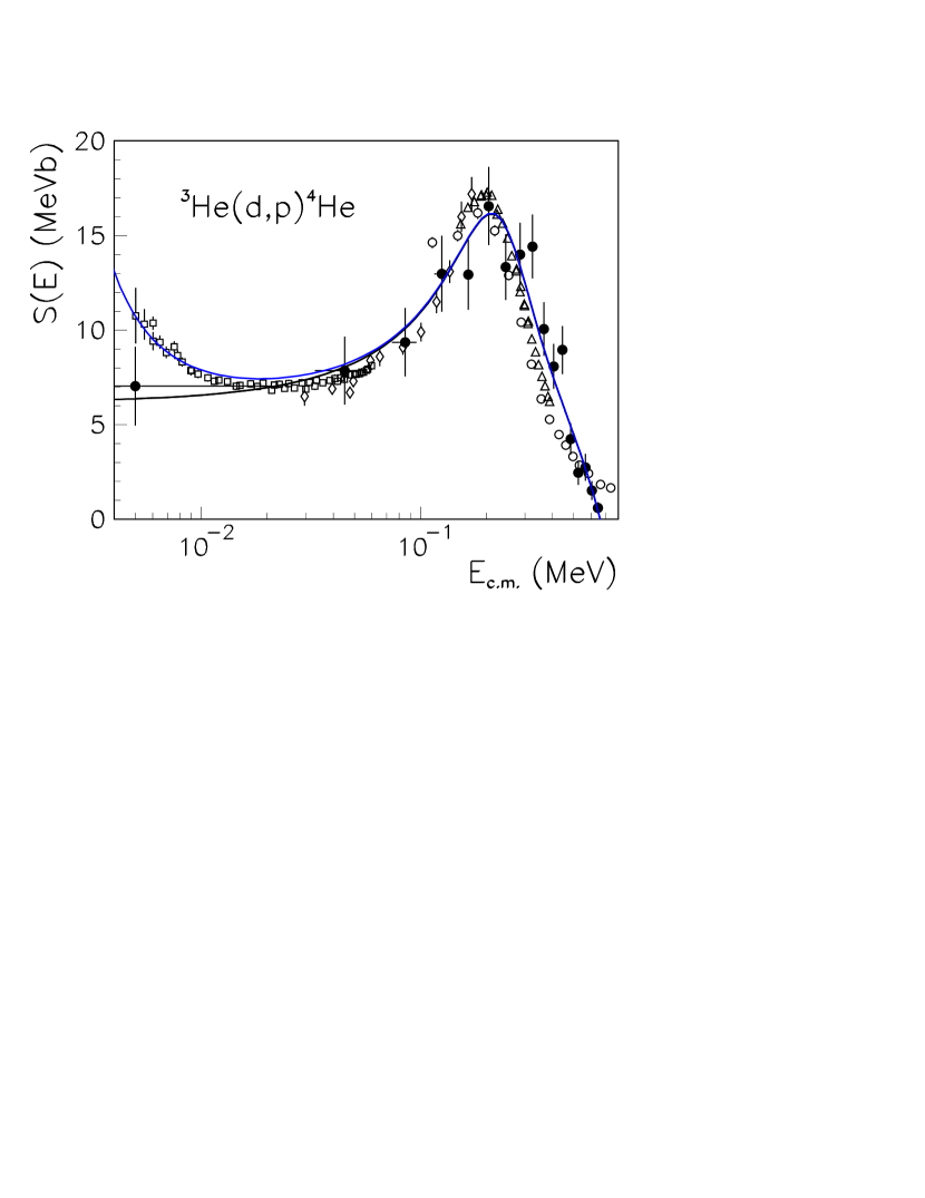
Figure 3: The ${}^{3}{\rm He}(d,p){}^{4}{\rm He}$ astrophysical $S$ factor determined from the TH reaction. The open circles and open triangles are direct experimental data; the full dots are the TH data. The black solid line represents the behavior of the bare nucleus S(E)-factor, resulting from a fit on the TH data, while the solid blue line is interpolation of the direct data.

III.1 TH reaction amplitude

A simple mechanism describing the TH process is the so-called QF process shown in Fig. 4.

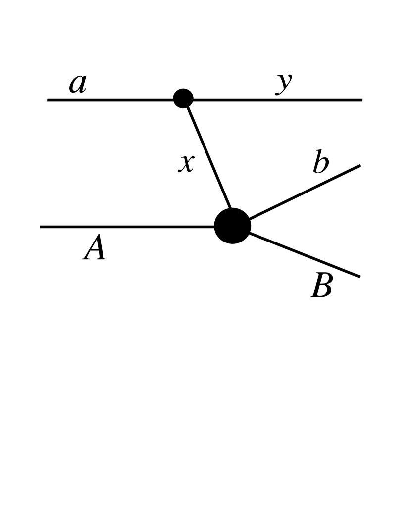
Figure 4: Pole diagram describing the quasi-free mechanism.

In the quasi-free process it is assumed that the incident particle (assume incident particle is $A$) interacts with one of the fragments of $a=(xy)$, say with $x$ which is considered to be ”quasifree”, while the second fragment is considered to be a ”passive” spectator which is not involved in the process. Thus the interaction of the spectator $y$ with $x$ and $A$ in the knockout process is neglected . The fact that the fragment $x$ is not free is taken into account by folding the quasi-free reaction amplitude with the Fourier component of the $(xy)$ bound-state wave function which takes into account the Fermi motion of $x$ in the bound state $a=(xy)$.

In this section we present a derivation of the TH reaction amplitude from the general $2\to 3$ reaction amplitude for the TH process (26). A general expression for the amplitude of the reaction is given by

$$M=<\chi_{bB}^{(-)}\chi_{yF}^{(-)}\varphi_{y}\varphi_{b}\varphi_{B}|\Delta V_{f}(1+G^{+}\Delta V_{i})|\varphi_{A}\varphi_{a}\chi_{i}^{(+)}>$$

(28)

$$=<\chi_{bB}^{(-)}\chi_{yF}^{(-)}\varphi_{y}\varphi_{b}\varphi_{B}|(\Delta V_{f}\,G^{+}+1)\Delta V_{i}|\varphi_{A}\varphi_{a}\chi_{i}^{(+)}>.$$

(29)

The amplitudes (28) and (29) are the post and prior forms of the exact amplitude. Let us consider the post form. Here, $G^{+}$ is the total Green function of the system $a+A$, $\,\chi^{(+)}_{i}$ is the distorted wave describing the scattering wave function of $a+A$ in the initial state of the reaction, $\chi^{(-)}_{bB}$ is the distorted wave describing the scattering of particles $b+B$ in the final state: the distorted wave $\chi^{-}_{yF}$ describes the distorted wave of the spectator $y$ and the center of mass of the system $F=b+B$ in the final state. For the moment we assume that Coulomb interactions are screened. Eventually we can take the limit of the screening radius to infinity. Also $\phi_{i}$ is the bound state wave function of nucleus $i$,

$$\Delta V_{i}=V_{aA}-U_{aA},$$ (30)

$$\Delta V_{f}=V_{bB}-U_{bB}+V_{yF}-U_{yF},$$ (31)

$V_{ij}$ and $U_{ij}$ are the interaction potential and optical potential between particles $i$ and $j$. For example, $V_{aA}=V_{xA}+V_{yA}$. To extract the amplitude of the subprocess $x+A\to b+B$, which is the final goal of the TH method, we note that the Hamiltonian of the system $a+A$ is

$$H=H_{aA}+H_{a}+H_{A}=H_{xA}+H_{yF}+H_{x}+H_{A}+H_{y},$$ (32)

where $H_{i}$ is the internal Hamiltonian of nucleus $i$ and $H_{ij}=T_{ij}+V_{ij}$ is the Hamiltonian of the relative motion of nuclei $i$ and $j$, $T_{ij}$ is their relative kinetic energy operator and $V_{ij}$ is their interaction potential. The total Green’s function operator can be written as

$$G^{+} = \frac{1}{E-H_{aA}-H_{a}-H_{A}+i0}$$ (36)

$$=\frac{1}{E-H_{xA}-H_{yF}-H_{xyA}^{0}+i0}$$

$$=\frac{1}{E-H_{xA}-T_{yF}-U_{yF}-\Delta{V}_{yF}-H_{xyA}^{0}+i0}$$

$$={\tilde{G}}^{+}+G^{+}\,\Delta V_{yF}\,{\tilde{G}}^{+},$$

Here $\Delta V_{f}=V_{yF}-U_{yF}$, $\,V_{yF}=V_{yx}+V_{yA}$,
$H_{xyA}^{0}=H_{x}+H_{y}+H_{A}$ and

$${\tilde{G}}^{+}=\frac{1}{E-H_{xA}-T_{yF}-U_{yF}-H_{xyA}^{0}+i0}$$ (37)

We substitute Eq. (37) into (28) and drop the term
$\Delta V_{f}\,G^{+}\,\Delta V_{yF}\,{\tilde{G}}^{+}\,\Delta V_{i}$ as the higher order term in the perturbation expansion over $\Delta V$. Then we get from Eq. (28)

$$M=<\chi_{bB}^{(-)}\chi_{yF}^{(-)}\varphi_{y}\varphi_{b}\varphi_{B}|\Delta V_{f}(1+{\tilde{G}}^{+}\,\Delta V_{i})|\varphi_{A}\varphi_{a}\chi_{i}^{(+)}>.$$

(38)

To single out the TH subprocess amplitude we replace $\Delta V_{i}=V_{xA}+V_{yA}-U_{aA}$ by $V_{xA}$ and $\Delta V_{f}=V_{yF}-U_{yF}+V_{bB}-U_{bB}$ by $\Delta V_{bB}=V_{bB}-U_{bB}$. Then the amplitude (28) becomes

$$M=<\chi_{bB}^{(-)}\chi_{yF}^{(-)}\varphi_{y}\varphi_{b}\varphi_{B}|\Delta V_{bB}\,(1+{\tilde{G}}^{+}\,V_{xA})|\varphi_{A}\varphi_{a}\chi_{i}^{(+)}>$$

$$=<\chi_{bB}^{(-)}\chi_{yF}^{(-)}\varphi_{y}\varphi_{b}\varphi_{B}|\Delta V_{bB}\,(1+G^{+}_{xA}\,V_{xA})|\varphi_{A}\varphi_{a}\chi_{i}^{(+)}>.$$

(39)

Here

$$G^{+}_{xA}=\frac{1}{E_{xA}-H_{xA}+i0}$$ (40)

and $E_{xA}$ is the relative kinetic energy of particles $x$ and $A$. The appearance of $G^{+}_{xA}$ in Eq. (40) is due to

$$<\chi_{yF}^{(-)}\varphi_{y}\varphi_{b}\varphi_{B}|{\tilde{G}}^{+}=<\chi_{yF}^{(-)}\varphi_{y}\varphi_{b}\varphi_{B}|G^{+}_{xA}.$$ (41)

Eq. (39) reveals a very important result. It contains a factor $1+G^{+}_{xA}\,V_{xA}$. For the on-shell case, the relative momentum of particles $x$ and $A\;{\rm{\bf p}}_{xA}={\rm{\bf k}}_{xA}$, where ${\rm{\bf k}}_{xA}$ is the $x-A$ on-shell relative momentum related with their relative kinetic energy as $E_{xA}=p_{xA}^{2}/(2\,\mu_{xA})$. Correspondingly,

$$(1+G^{+}V_{xA})|e^{i{\rm{\bf k}}_{xA}\cdot{\rm{\bf r}}_{xA}}>=\chi_{{\rm{\bf k}}_{xA}}^{+}({\rm{\bf r}}_{xA}).$$ (42)

is the scattering wave function of particles $x$ and $A$ interacting via the optical potential $V_{xA}$. We assume at the moment that all the Coulomb interactions are screened. However, in the TH method the entry particle $x$ is not free because it is in the bound state $a=(xy)$, i. e. the momentum of $x$ is not fixed. In other words, $x$ is off-the-energy shell because $E_{xA}\not=p_{xA}^{2}/(2\,\mu_{xA})$. For the off-shell case

$$(1+G^{+}V_{xA})|e^{i{\rm{\bf p}}_{xA}\cdot{\rm{\bf r}}_{xA}}>=\chi_{(os){\rm{\bf k}}_{xA},{\rm{\bf p}}_{xA}}^{+}({\rm{\bf r}}_{xA})$$ (43)

is the so-called off-shell scattering function,

III.2 TH method for direct reactions

We first consider the direct subreaction (27). We assume that this reaction proceeds through the transfer of particle $c$ from $A$ to $x$ (it can be also considered as a particle transfer from $x$ to $A$), i. e. $A=(Bc)$ and $b=(xc)$. The ”pole” diagram corresponding to the on-shell reaction describing the particle $c$ transfer mechanism with the $x-A$ rescattering in the initial and $b-B$ rescattering in the final state is shown in Fig. 5. This diagram describes the DWBA amplitude.

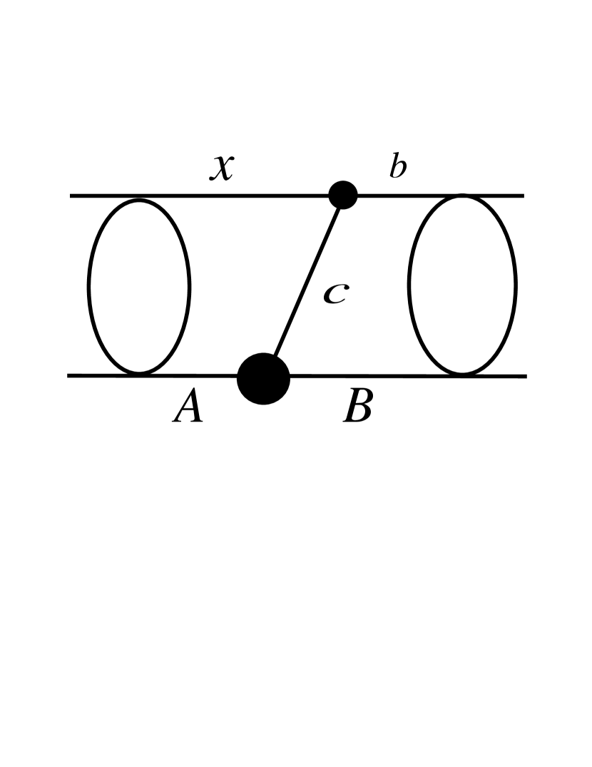
Figure 5: Pole diagram describing the direct reaction $x+A\to b+B$ mechanism. Bubbles show the initial and final state interactions.

To simplify Eq. (39) in the case of the direct transfer subprocess, we insert the projection operators $\sum\varphi_{x}><\varphi_{x}$, $\,\sum\varphi_{B}><\varphi_{B}$ and $\sum\varphi_{c}><\varphi_{c}$ into the bra and ket states. The sum is taken over discrete states and an integral is used for the continuum states of the corresponding nucleus. We leave in the projection operator only the ground state projections $\varphi_{x}><\varphi_{x}$, $\,\varphi_{B}><\varphi_{B}$ and $\varphi_{c}><\varphi_{c}$ assuming that only the ground states of $x$, $B$ and $c$ contribute to the reaction. If necessary the excited states can also be taken into account. Then we get

$$<\varphi_{y}\varphi_{b}\varphi_{B}|\Delta V_{bB}\,(1+G^{+}_{xA}\,V_{xA})|\varphi_{A}\varphi_{a}>$$

$$\approx<\varphi_{b}|\varphi_{c}\varphi_{x}><\varphi_{B}|\Delta V_{bB}|\varphi_{B}>$$

$$\times(1+<\varphi_{x}|G^{+}_{xA}|\varphi_{x}><\varphi_{x}|V_{xA}|\varphi_{x}>)$$

$$<\varphi_{c}\varphi_{B}|\varphi_{A}><\varphi_{x}\varphi_{y}|\varphi_{a}>$$ (44)

We introduce the overlap functions $I^{\alpha}_{\beta\gamma}=<\varphi_{\beta}\,\varphi_{\gamma}|\varphi_{\alpha}>$ and use the approximation $\,<\varphi_{x}|V_{xA}|\varphi_{x}>\,\approx U_{xA}$; also we use the approximation

$$<\varphi_{x}|G^{+}_{xA}|\varphi_{x}>\approx G^{(U)+}_{xA}={(E_{xA}-T_{xA}-U_{xA}+i0)}^{-1}.$$

(45)

Note that $<\varphi_{B}|\Delta V_{bB}|\varphi_{B}>\approx V_{xB}+V_{cB}-U_{bB}$, where $V_{jB}$ is the interaction potential between the point like nuclei $j=x,c$ and $B$. All the neglected terms are higher order in the perturbation theory over $\Delta V$. Then we get in lowest order for the TH amplitude with the subprocess described by the direct transfer reaction (27):

$$M=<\chi_{yF}^{(-)}[\chi_{bB}^{(-)}I^{b}_{xc}|\Delta V_{bB}|\,I^{A}_{cB}\,(1+G^{+}_{xA}\,V_{xA})]\,I^{a}_{xy}\chi_{i}^{(+)}>.$$

(46)

The expression in the brackets is the amplitude of subreaction (27) which is the final goal of the TH. To see it we just rewrite (46) in momentum space:

$$M = \int\frac{{\rm d}{\rm{\bf p}}_{yF}}{(2\,\pi)^{3}}\,\frac{{\rm d}{\rm{\bf p}}_{xA}}{(2\,\pi)^{3}}\,\chi_{yF}^{*(-)}({\rm{\bf p}}_{yF})\,M^{sub}({\rm{\bf k}}_{bB},{\rm{\bf p}}_{xA})\,I^{a}_{xy}({\rm{\bf p}}_{xy})\,$$ (47)

$$\times\chi_{i}^{(+)}({\rm{\bf p}}_{xA}),$$

where

$${\rm{\bf p}}_{xy}=\frac{m_{y}{\rm{\bf p}}_{x}-m_{x}{\rm{\bf p}}_{y}}{m_{x}+m_{y}}=\frac{m_{y}}{m_{x}}{\rm{\bf p}}_{a}-{\rm{\bf p}}_{y}.$$ (48)

Also note that in the center of mass of TH reaction $a+A\to y+b+B$ the relative momentum is given by ${\rm{\bf p}}_{aA}={\rm{\bf p}}_{a}$ and ${\rm{\bf p}}_{yF}={\rm{\bf p}}_{y}$. We denote by ${\rm{\bf p}}_{i}$ $\;({\rm{\bf k}}_{i})$ the momentum of the virtual (real) particle $i$ and by $\;({\rm{\bf k}}_{ij})$ the relative momentum of virtual (real) particles $i$ and $j$. Also $\chi_{i}^{(+)}({\rm{\bf p}}_{xA})\equiv\chi_{{\rm{\bf k}}_{aA}}^{(+)}({\rm{\bf p}}_{xA})$, i. e. it is the Fourier component of the $a-A$ scattering wave function with the incident momentum ${\rm{\bf k}}_{aA}$ which in the center of mass of the TH reaction is just ${\rm{\bf k}}_{a}$. Correspondingly $\chi_{yF}^{(-)}({\rm{\bf p}}_{yF})\equiv\chi_{{\rm{\bf k}}_{yF}}^{(-)}({\rm{\bf p}}_{yF})$.

The half-off-the-energy shell amplitude of the subprocess (27) is given by

$$M^{sub}({\rm{\bf k}}_{bB},{\rm{\bf p}}_{xA})=<\chi_{bB}^{(-)}I^{b}_{xc}|\Delta V_{bB}|\,I^{A}_{cB}\,\chi_{(os){\rm{\bf k}}_{xA},{\rm{\bf p}}_{xA}}^{+}>.$$

(49)

The virtuality of the entry particle $x$ of this amplitude results in the fact that the relative momentum of particles $x$ and $A$ in the initial state of reaction (27) $p_{xA}\not=\sqrt{2\,\mu_{xA}\,E_{xA}}$. Due to the off-shell entry particles amplitude (49) does not have the Gamow penetration factor. We would like to underscore that from $E_{xA}+Q=E_{bB}$ for positive $Q>0$ for reaction (27) at $E_{xA}\to 0$, $\,E_{bB}\approx{\rm const}$. Hence the off-shell scattering function $\chi_{(os){\rm{\bf k}}_{xA},{\rm{\bf p}}_{xA}}^{+}$ is the only $E_{xA}$ dependent factor in $M^{sub}$ at $E_{xA}\to 0$. The off-shell scattering function is a universal factor which does not depend on the specifics of the direct reaction. Rewritting matrix element in Eq. (49) in the momentum representation gives

$$M^{sub}({\rm{\bf k}}_{bB},{\rm{\bf p}}_{xA})=\int\frac{{\rm d}{\rm{\bf p}}_{bB}}{(2\,\pi)^{3}}\,\frac{{\rm d}{\rm{\bf p}}^{{}^{\prime}}_{xA}}{(2\,\pi)^{3}}\chi_{{\rm{\bf k}}_{bB}}^{*(-)}({\rm{\bf p}}_{bB})$$

$$\times I^{*b}_{xt}({\rm{\bf p}}^{{}^{\prime}}_{x}-\frac{m_{x}}{m_{b}}\,{\rm{\bf p}}_{b})\,\Delta V_{bB}\,I^{A}_{cB}({\rm{\bf p}}_{B}-\frac{m_{B}}{m_{A}}\,{\rm{\bf p}}^{{}^{\prime}}_{A})$$

$$\times\chi_{(os){\rm{\bf k}}_{xA},{\rm{\bf p}}_{xA}}^{+}({\rm{\bf p}}^{{}^{\prime}}_{xA})$$ (50)

Approximation $\Delta V_{bB}\approx V_{cB}$, which works for $m_{x}>m_{c}$, is enough for us to investigate the dependence of
$M^{sub}({\rm{\bf k}}_{bB},{\rm{\bf p}}_{xA})$ on $E_{xA}$ for arbitrary masses of $x$ and $c$. Using this approximation we get from Eq. (50)

$$M^{sub}({\rm{\bf k}}_{bB},{\rm{\bf p}}_{xA})=\int\frac{{\rm d}{\rm{\bf p}}_{bB}}{(2\,\pi)^{3}}\,\frac{{\rm d}{\rm{\bf p}}^{{}^{\prime}}_{xA}}{(2\,\pi)^{3}}\chi_{{\rm{\bf k}}_{bB}}^{*(-)}({\rm{\bf p}}_{bB})$$

$$\times I^{*b}_{xc}({\rm{\bf p}}^{{}^{\prime}}_{x}-\frac{m_{x}}{m_{b}}\,{\rm{\bf p}}_{b})\,W^{A}_{cB}({\rm{\bf p}}_{B}-\frac{m_{B}}{m_{A}}\,{\rm{\bf p}}^{{}^{\prime}}_{A})$$

$$\times\chi_{(os){\rm{\bf k}}_{xA},{\rm{\bf p}}_{xA}}^{+}({\rm{\bf p}}^{{}^{\prime}}_{xA}).$$ (51)

Here $W^{A}_{cB}({\rm{\bf p}}_{cB})$ is the form factor determined by

$$W^{A}_{cB}({\rm{\bf p}}_{cB})=\int{\rm d}{\rm{\bf r}}_{cB}e^{-i\,{\rm{\bf p}}_{cB}\cdot{\rm{\bf r}}_{cB}}\,V_{cB}(r_{cB})\,I^{A}_{cB}({\rm{\bf r}}_{cB}).$$ (52)

The Fourier component of the off-shell scattering function $\chi_{(os){\rm{\bf k}}_{xA},{\rm{\bf p}}_{xA}}^{+}({\rm{\bf r}}_{xA})$ is given by

$$\chi_{(os){\rm{\bf k}}_{xA},{\rm{\bf p}}_{xA}}^{+}({\rm{\bf p}}^{{}^{\prime}}_{xA}) = \delta({\rm{\bf p}}^{{}^{\prime}}_{xA}-{\rm{\bf p}}_{xA})+G^{+}_{0}(p^{{}^{\prime}}_{xA};E_{xA})$$ (53)

$$\times T({\rm{\bf p}}^{{}^{\prime}}_{xA},{\rm{\bf p}}_{xA};E_{xA}),$$

$$G^{+}_{0}(p^{{}^{\prime}}_{xA};E_{xA})=\frac{1}{E_{xA}-p_{xA}^{{}^{\prime}2}/2\,\mu_{xA}+i0},$$ (54)

$T({\rm{\bf p}}^{{}^{\prime}}_{xA},{\rm{\bf p}}_{xA};E_{xA})$ is the off-shell $x-A$ scattering amplitude. Amplitude $M^{sub}({\rm{\bf k}}_{bB},{\rm{\bf p}}_{xA})$ extracted from the THM should be compared with the corresponding on-shell reaction amplitude

$$M^{onsh}({\rm{\bf k}}_{bB},{\rm{\bf k}}_{xA})=\int\frac{{\rm d}{\rm{\bf p}}_{bB}}{(2\,\pi)^{3}}\,\frac{{\rm d}{\rm{\bf p}}_{xA}}{(2\,\pi)^{3}}\chi_{{\rm{\bf k}}_{bB}}^{*(-)}({\rm{\bf p}}_{bB})$$

$$\times I^{*b}_{xt}({\rm{\bf p}}_{x}-\frac{m_{x}}{m_{b}}\,{\rm{\bf p}}_{b})\,\Delta V_{bB}\,I^{A}_{cB}({\rm{\bf p}}_{B}-\frac{m_{B}}{m_{A}}\,{\rm{\bf p}}_{A})$$

$$\times\chi_{{\rm{\bf k}}_{xA}}({\rm{\bf p}}_{xA})$$ (55)

Eqs. (47) and (49) is our final result. The diagram corresponding to this amplitude (47) is shown in Fig. 6.

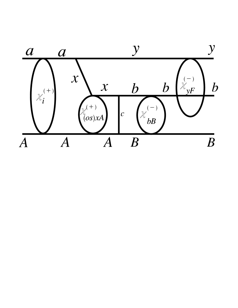
Figure 6: Diagram describing the TH reaction $a+A\to y+b+B$ proceeding through the direct subprocess $x+A\to b+B$ mechanism. Bubbles show initial and final state interactions and the off-shell scattering function.

Eq. (47) is a general expression for the TH reaction amplitude which contains the half-off-shell direct subprocess amplitude and the initial and final state rescatterings. As we can see the subprocess amplitude is not factorized, but instead is folded with the initial and final state distorted waves and the overlap function for $a\to y+x$. Note that if the initial and distorted waves in the momentum space are replaced by delta-functions, Eq. (47) just becomes a trivial plane wave impulse approximation described by the diagram of Fig. 3.

III.3 TH for resonant reactions

In Subsection III.1 we derived a general expression, Eq. (39), for the amplitude of the TH reaction (26) which is valid for both direct and resonant subprocesses (27). Here we consider the resonant TH reactions, i. e. we assume that the subprocess (27) proceeds through the intermediate resonance $F^{*}$. Our goal is to relate the half-off-shell and on-shell resonant amplitudes. Note that it is easier to relate the off-shell and on-shell resonant reactions than the direct ones. The resonant TH amplitude can be extracted from Eq. (39) in a straightforward manner because it contains the Green’s operator $G^{+}_{xA}$. Below we demonstrate how to do it. For simplicity here we neglect the initial and final state interactions.

The TH amplitude of the reaction (26), which proceeds through the resonance state $F^{*}$ in the intermediate system $x+A$, is given by

$$M=M^{sub(R)}({\rm{\bf k}}_{bB},{\rm{\bf p}}_{xA})\,I^{a}_{xy}({\rm{\bf p}}_{xy}).$$ (56)

Here $M^{sub(R)}$ is the amplitude of the resonant subprocess (27). Usually in practical calculations the overlap function $I^{a}_{xy}$ is expressed in terms of the corresponding single-particle bound state wave function $\varphi_{xy}$:

$$I^{a}_{xy}=S_{xy}^{1/2}\,\varphi_{xy}.$$ (57)

Here, $S_{xy}$ is the spectroscopic factor of the bound state $(xy)$ in $a$ with given quantum numbers. For simplicity we don’t write down symbols corresponding to the quantum numbers and assume that $S_{xy}=1$. In the momentum space the bound state wave function is given by

$$\varphi_{xy}({\rm{\bf p}}_{xy})\,=-2\mu_{xy}\frac{{W({\rm{\bf p}}_{xy})\,}}{{p_{xy}^{2}\,+\,\kappa_{xy}^{2}}},$$ (58)

$$W({\rm{\bf p}}_{xy})=\,\int{d{\rm{\bf r}}}\,e^{-i{\rm{\bf p}}_{xy}\cdot{\rm{\bf r}}}\,V_{xy}(r)\,\varphi_{xy}({\rm{\bf r}})$$ (59)

$$=(-\varepsilon_{a}-\frac{{p_{xy}^{2}}}{{2\mu_{xy}}}\,)\,\varphi_{xy}({\rm{\bf p}}_{xy}),$$ (60)

Now we can find the virtuality factor

$$\sigma_{x}=E_{x}-\frac{{p_{x}^{2}}}{{2m_{x}}}.$$ (61)

of the virtual particle $x$ using the energy and momentum conservation laws in both vertices $a\to x+y$ and $x+A\to F^{*}$. After simple algebraic transformations we get

$$\sigma_{x}=E_{xA}-\frac{{p_{xA}^{2}}}{{2\mu_{xA}}}=-\frac{1}{{2\mu_{xy}}}[p_{xy}^{2}+(\kappa_{xy}^{a})^{2}]\,<0.$$ (62)

Thus we derived a very important result for the relative kinetic energy of particles $x$ and $A$ $\,E_{xA}$ in the TH method: $\;E_{xA}<p_{xA}^{2}/2\mu_{xA}$, i. e. always $k_{xA}<p_{xA}$, where $k_{xA}=\sqrt{2\,\mu_{xA}\,E_{xA}}$ is the $x-A$ relative on-shell momentum. The half-off-shell resonant reaction amplitude in the TH method is described by the diagram shown in Fig. 7

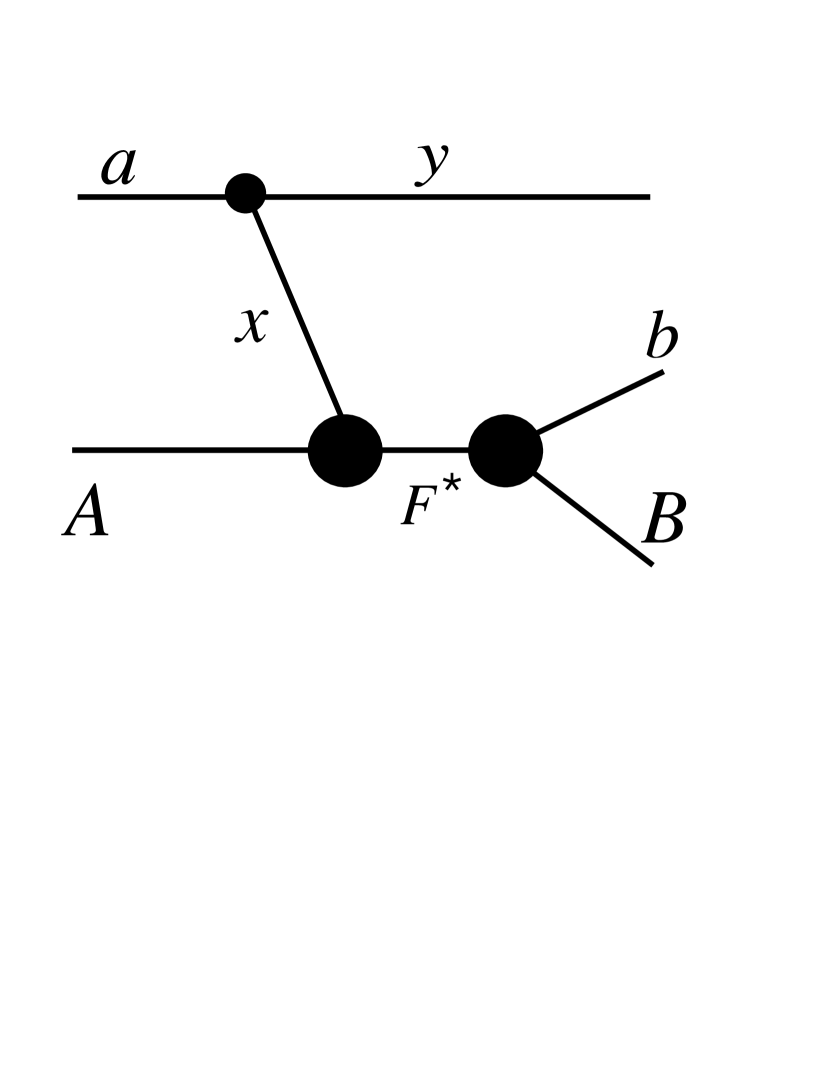
Figure 7: Diagram describing the resonant reaction $a+A\to y+b+B$.

and is given by

$$M^{sub(R)}({\rm{\bf k}}_{bB},\,{\rm{\bf p}}_{xA};E)=-\frac{1}{2}(4\pi)^{2}\,\sqrt{\frac{1}{{\mu_{bB}k_{bB}}}}$$

$$\sum\limits_{m_{0}=-l_{0}}^{l_{0}}{Y_{l_{0}m_{0}}}(\hat{\rm{\bf k}}_{bB}Y_{l_{0}m_{0}}^{*}(\hat{\rm{\bf p}}_{xA})\,e^{i\delta_{fl_{0}}(k_{bB})}$$

$$\frac{{\sqrt{\Gamma_{bB}(E_{bB},r_{0})}\,w_{l_{0}}(p_{xA},k_{xA(R)})}}{{E_{xA}-E_{xA}^{(R)}}}.$$

(63)

Here $k_{xA(R)}=\sqrt{2\,\mu_{xA}\,E_{xA}^{(R)}}$, $\,{\rm{\bf k}}_{bB}$ is the on-shell relative momentum of particles $b$ and $B$ in the final state, $l_{0}(m_{0})$ is the resonance orbital angular momentum (its projection), $Y_{l_{0}m_{0}}$ is the corresponding spherical harmonics, $\hat{\rm{\bf r}}={\rm{\bf r}}/r$, $\,\delta_{fl_{0}}$ is the nonresonant (potential) scattering phase shift of particles $b$ and $B$ in the final state. The off-shell form factor

$$w_{l_{0}}(p_{xA},k_{xA(R)})=\int\limits_{0}^{\infty}{dr\,r^{2}\psi_{nl_{0}}^{(R)}(r)}\,V(r)j_{l_{0}}(p_{xA}\,r)$$

$$=(E_{xA}^{(R)}-E_{p_{xA}})\int\limits_{0}^{\infty}{dr\,r^{2}\psi_{nl_{0}}^{(R)}(r)}\,j_{l_{0}}(p_{xA}\,r)$$

$$=(E_{xA}^{(R)}-E_{p_{xA}})\,\psi_{nl_{0}}^{(R)}(p_{xA}).$$

(64)

Here $\psi_{nl_{0}}^{(R)}(r)$ is the resonant Gamow radial wave function, $\psi_{nl_{0}}^{(R)}(p_{xA})$ is its Fourier component, $j_{l_{0}}(p_{xA}\,r)$ is the spherical Bessel function, $E_{p_{xA}}=p_{xA}^{2}/2\,\mu_{xA}$, $n$ is the principal quantum number.

Let us write down the well known expression for the on-shell Breit-Wigner resonance amplitude for the resonant process $x+A\to b+B$

$$M^{(R)}({\rm{\bf k}}_{bB},\,{\rm{\bf k}}_{xA};E)\,=-\frac{1}{4}(4\pi)^{2}\,\sqrt{\frac{1}{{\mu_{bB}k_{bB}}}}\sqrt{\frac{1}{{\mu_{xA}k_{xA}}}}$$

$$\times\sum\limits_{m_{0}=l_{0}}^{l_{0}}{Y_{l_{0}m_{0}}}(\hat{\rm{\bf k}}_{bB})Y_{l_{0}m_{0}}^{*}(\hat{\rm{\bf k}}_{xA})\,e^{i\delta_{fl_{0}}(k_{bB})}e^{i\delta_{fl_{0}}(k_{xA})}$$

$$\times\frac{{\sqrt{\Gamma_{bB}(E_{bB},r_{0})}\,\sqrt{\Gamma_{bB}(E_{xA},r_{0})}}}{{E_{xA}-E_{xA}^{(R)}}},$$

(65)

where ${\rm{\bf k}}_{xA}$ is the on-shell relative momentum of the initial particles $x$ and $A$ and ${\rm{\bf k}}_{bB}$ is the on-shell relative momentum of the final particles $b$ and $B$. In the $R$-matrix method the resonance width contains the Coulomb-centrifugal barrier penetrability factor which exponentially decreases with energy. Hence for $E_{xA}\to 0$ the resonant amplitude $M^{R}\sim\sqrt{P_{l_{0}}(k_{xA})}\,{\tilde{M}}^{R}$. Just this factor makes it difficult or impossible to measure resonant reactions at astrophysically relevant energies. Now we compare the half-off-shell resonant amplitude, Eq. (63), and the on-shell amplitude, Eq. (65). The half-off-shell amplitude contains the form factor
$w_{l_{0}}(p_{xA},k_{(xA)R})$. The barrier factor should come from the integral representation in Eq. (64), namely from $j_{l_{0}}(p_{xA}r)$. However, $j_{l_{0}}(p_{xA}r)$ does not contain the Coulomb penetration factor and does not depend on the on-shell momentum $k_{xA}$. Hence in limit $k_{xA}\to 0$ the off-shell form factor does not go to zero. We underscore that it is very important that always in the TH reaction $p_{xA}>k_{xA}$. Comparing Eqs (63) and (65) we get

$$M^{(R)}({\rm{\bf k}}_{bB},\,{\rm{\bf k}}_{xA};E_{xA})\,=-\frac{1}{2}e^{i\delta_{(xA)l_{0}}(k_{xA})}\sqrt{\frac{1}{{\mu_{xA}k_{xA}}}}$$

$$\times\frac{{\sqrt{\Gamma_{xA}(E_{xA},r_{0})}}}{{w_{l_{0}}(p_{xA},k_{xA(R)})}}M^{sub(R)}({\rm{\bf k}}_{bB},\,{\rm{\bf p}}_{xA};E_{xA}).$$ (66)

Note the only difference between the half-off-shell and the on-shell resonant amplitudes is the appearance of the form factor $w_{l_{0}}(p_{xA},k_{xA(R)})$. Now we give the expression for the on-shell resonant cross section which can be derived from the TH half-off-shell resonant cross section

$$\sigma(E_{xA})=\,\frac{{\mu_{xA}k_{xA}\,\mu_{bB}k_{bB}}}{{(2\pi)^{2}}}\,\frac{1}{{k_{xA}^{2}}}\frac{1}{{4\pi}}\int{{\rm d}\Omega_{{\rm{\bf k}}_{bB}}}$$

$$\times\int{{\rm d}\Omega_{{\rm{\bf k}}_{xA}}}|M^{(R)}({\rm{\bf k}}_{bB},\,{\rm{\bf k}}_{xA};E_{xA})\,\,|^{2}$$ (67)

$$=\frac{1}{4}\frac{{\,\mu_{bB}k_{bB}}}{{(2\pi)^{2}}}\frac{1}{{k_{xA}^{2}}}\frac{1}{{4\pi}}\frac{{\Gamma_{xA}(E_{xA},r_{0})}}{{|w_{l_{0}}(p_{xA},k_{xA(R)})|^{2}}}$$

$$\times\int{{\rm d}\Omega_{{\rm{\bf k}}_{bB}}\,}\int{{\rm d}\Omega_{{\rm{\bf p}}_{xA}}}|M^{sub(R)}({\rm{\bf k}}_{bB},\,{\rm{\bf p}}_{xA};E_{xA})\,|^{2}.$$ (68)

IV Summary

In this work we have addressed two important indirect techniques in nuclear astrophysics use, asymptotic normalization coefficient (ANC) and Trojan Horse (TH)
method. Both techniques allow one to determine the astrophysical factors at Gamow peak or even at zero energy avoiding extrapolation procedure. The ANC method determines the overall normalization of the peripheral radiative capture processes. The ANC technique becomes especially powerful for astrophysical processes proceeding through a subthreshold state - a loosely bound state. In this case the ANC determines both the overall normalization of the direct radiative capture to the subthreshold state and the resonance partial width for captures through the subthreshold resonance. We demonstrated the application of the ANC technique for the key CNO cycle reaction ${}^{14}{\rm N}(p,\,\gamma){}^{15}{\rm O}$. The ANC method turns out to be useful also for determination of the sign of the interference term of the resonant and nonresonant radiative capture amplitudes. We demonstrated it for two important CNO cycle reactions: ${}^{11}{\rm C}(p,\,\gamma){}^{12}{\rm N}$ and ${}^{13}{\rm N}(p,\,\gamma){}^{14}{\rm O}$.

The TH method allows one to determine the astrophysical factors for astrophysical reactions, both direct and resonant. In practical applications the astrophysical factor extracted from the TH reaction is available in a wide energy range from astrophysical energies to higher energies. Its absolute normalization is determined by normalization of the TH astrophysical factor to the one obtained from direct measurements at higher energies. Assuming that the energy dependence of the TH astrophysical factor is correct, one can determine the absolute astrophysical factor at astrophysical energies. In this work we have derived a general expression for the TH reaction amplitude which takes into account the off-shell effects and initial and final state interactions. The direct and resonant TH reactions are considered separately. We derived the TH amplitude for direct subreactions in terms of the off-shell scattering wave function. The energy dependence of this wave function determines the energy dependence of the TH astrophysical factor for an arbitrary direct reaction mechanism. We connect the TH resonant cross section with the on-shell resonant cross section. We intend to use the derived equations to calculate the absolute astrophysical factors.

References

• (1) C. Rolfs and W. S. Rodney, Cauldrons in the Cosmos, (The University of Chicago Press, 1988), 368.
• (2) H. J. Assenbaum, K. Langanke, and C. Rolfs, Z. Phys. A 327, (1987) 461.
• (3) F. Streider et al., Naturwissenschaften 88, (2001) 461.
• (4) C. Casella et al., Luna Collaboration, Nucl. Phys. A706, (2002) 203.
• (5) C. Spitaleri et al., Phys. Rev. C 69, (2004) 055806.
• (6) A. M. Mukhamedzhanov et al., Phys. Rev. C 67, (2003) 065804.
• (7) G. Baur et al., Nucl. Phys. A458, (1986) 188.
• (8) T. Motobayashi et al., Phys. Rev. Lett. 73, (1994) 2680.
• (9) G. Baur, Phys. Lett. B 178, (1986) 135.
• (10) W. Younes and H. C. Britt, Phys. Rev. C 67, (2003) 024610.
• (11) A. M. Mukhamedzhanov and N. K. Timofeyuk, JETP. Lett. 51, (1990) 282.
• (12) H. M. Xu et al., Phys. Rev. Lett. 73, (1994) 2027.
• (13) C. A. Gagliardi et al., Phys. Rev. C 59, (1999) 1149.
• (14) A. M. Mukhamedzhanov, R. E. Tribble, Phys. Rev. C 59, (1999) 3418.
• (15) L. D. Blokhintsev, I. Borbely and E. I. Dolinskii, Fiz. Elem. Chastits At. Yadra 8, (1977) 1189. C 59, (1999) 3418
• (16) L. D. Blokhintsev et al., Phys. Rev. C 48, (1993) 2390.
• (17) P. F. Bertone et al., Phys. Rev. C 66, (2002) 055804.
• (18) U. Schröder et al., Nucl. Phys. A 467, (1987) 240.
• (19) A. Formicola et al., Phys. Lett. B 591, (2004) 61.
• (20) P. F. Bertone et al., Phys. Rev. Lett. 87, (2001) 152501.
• (21) F. C. Barker, T. Kajino, Aust. J. Phys. 44, (1991) 369.
• (22) X.D. Tang et al., Phys. Rev. C 67, (2003) 015804.
• (23) T. Minemura et al., RIKEN Accel. Prog. Rep. A35, (2002).
• (24) P. Descouvemont, Nucl. Phys. A646, (1999) 261.
• (25) M. Wiescher et al., Astrophys. J. 343, (1989) 352.
• (26) X. D. Tang et al., Phys. Rev. C 69, (2004) 055807.
• (27) P. Descouvemont and D. Baye, Nucl. Phys. A500, (1989) 155.
• (28) P. Descouvemont, Nucl. Phys. A646, (1999) 261.
• (29) C. J. Copi, D. N. Schramm, and M. S. Turner, Scand. J. Immunol. 627, (1995) 192.
• (30) L. Piau and S. Turck-Chieze, Astrophys. J. 566, (2002) 419.
• (31) A. Tumino et al., Phys. Rev. C 67, (2003) 065803.
• (32) M. La Cognata et al., Nucl. Phys. A (2005) (in press).