Abstract

We outline the structure of the nuclear force in the framework of chiral effective field theory of QCD and review recent applications to processes involving few nucleons.

Keywords: effective field theory, chiral perturbation theory, nuclear forces, few–nucleon systems, isospin–violating effects, chiral extrapolations.

1 Introduction

One of the basic problems in nuclear physics is determining the nature of the interactions between the nucleons which is crucial for understanding the properties of nuclei. The standard way to describe the nuclear force is based on the meson–exchange picture, which goes back to the seminal work by Yukawa [1]. His idea as well as experimental discovery of $\pi$– and heavier mesons ($\rho$, $\omega$, $\dots$) stimulated the development of boson–exchange models of the nuclear force, which still provide a basis for many modern, highly sophisticated phenomenological nucleon–nucleon (NN) potentials.

According to our present understanding, the nuclear force is due to residual strong interactions between the color–charge neutral hadrons. A direct derivation of the nuclear force from QCD, the underlying theory of strong interactions, is not yet possible due to its nonperturbative nature at low–energy. In order to provide reliable input for few– and many–body calculations, research on the NN interaction proceeded along (semi-)phenomenological lines with the aim of achieving the best possible description of the low–energy NN data. In the case of two nucleons, the potential can be decomposed in a few different spin–space structures, and the corresponding radial functions can be parameterized using an extensive set of data. Although the resulting models provide an excellent description of experimental data in many cases, there are certain major conceptual deficiencies that cannot be overcome. In particular, one important concern is related to the problem of the construction of consistent many–body forces. These can only be meaningfully defined in a consistent scheme with a given two–nucleon (2N) interaction [2]. Notice that because of the large variety of different possible structures in the three–nucleon force (3NF), following the same phenomenological path as in the 2N system and parametrizing the most general structure of the 3NF seems not to be feasible without additional theoretical guidance. Clearly, the same problem of consistency arises in the context of reactions with electroweak probes, whose description requires the knowledge of the corresponding consistent nuclear current operator. Further, one lacks within phenomenological treatments a means of systematically improving the theory of the nuclear force in terms of the dominant dynamical contributions. Finally, and most important, the phenomenological scheme provides only loose connection to QCD.

Chiral Effective Field Theory (EFT) has become a standard tool for analyzing the properties of hadronic systems at low energies in a systematic and model independent way. It is based upon the approximate and spontaneously broken chiral symmetry of QCD, which governs low–energy hadron structure and dynamics. In addition, it provides a straightforward way to improve the results by going to higher orders in a perturbative expansion. In the past two decades, this framework was successfully applied to a variety of low–energy reactions in the meson and single–baryon sectors. Fifteen years ago Weinberg [3, 4] proposed a generalization of this approach to the few–nucleon sector, where one has to deal with a nonperturbative problem. He demonstrated that the strong enhancement of the few–nucleon scattering amplitude arises from purely nucleonic intermediate states and suggested to apply EFT to the kernel of the corresponding scattering equation, which can be viewed as an effective nuclear potential. This idea has been explored in the last decade by many authors. In this work, we will review the current status of research along these lines, focusing on the description of few–nucleon systems. The manuscript is organized as follows. In section 2 we discuss effective field theories which are of relevance for the topics considered in this work. In particular, we give a brief account of chiral EFT for the pion and single–nucleon sectors and then discuss how it can be generalized to the few–nucleon sector. In section 3 we consider the structure of the nuclear force based on chiral EFT. Applications to systems with $2\ldots 7$ nucleons are presented in section 4. Section 5 lists some related further topics which are not covered in this work. A brief outlook is presented in section 6. Finally, appendix A contains explicit expressions for certain contributions to the 2N force.

2 Effective field theories in nuclear physics

2.1 Chiral perturbation theory

Chiral Perturbation Theory (CHPT) is the effective theory of QCD and, more generally, of the Standard Model, which was formulated by Weinberg [5] and developed in to a systematic tool for analyzing low–energy Quantum Chromodynamics (QCD) by Gasser and Leutwyler [6, 7]. In this section, we give a brief overview of the foundations of this approach.

Consider the QCD Lagrangian in the two–flavor case of the light up and down quarks

$$\mathcal{L}_{\rm QCD}=\bar{q}\,(i\gamma_{\mu}D^{\mu}-\mathcal{M})q-\frac{1}{4}G^{a}_{\mu\nu}G^{a\,\mu\nu}\,,$$ (2.1)

where $D_{\mu}=\partial_{\mu}-ig_{s}G_{\mu}^{a}T^{a}$ with $T^{a}$, (with $a=1\ldots 8$) are the SU(3)_color Gell–Mann matrices and $q$ the quark fields. Further, $G_{\mu\nu}^{a}$ are the gluon field strength tensors, and the quark mass matrix is given by $\mathcal{M}=\mbox{diag}(m_{u},\,m_{d})$. We do not show in Eq. (2.1) the $\theta$– and gauge fixing terms which are not relevant for our consideration. The left– and right–handed quark fields are defined by $q_{\rm L,R}=1/2(1\pm\gamma_{5})q$. The chiral group $G$ is a group of independent SU(2)_flavor transformations of the left– and right–handed quark fields, $G=$ SU(2)_L $\times$ SU(2)_R. Expressing the quark part in the QCD Lagrangian (2.1) in terms of $q_{L,R}$, it is easy to see that the covariant derivative term is invariant with respect to global chiral rotations, while the quark mass term is not. The running quark masses in the $\overline{\mbox{MS}}$ scheme at the renormalization scale $\mu=1$ GeV are $m_{u}\sim 5$ MeV and $m_{d}\sim 9$ MeV [8]. Given the fact that the masses of the up and down quarks are much smaller than the typical hadron scale of the order of 1 GeV, chiral SU(2)_L $\times$ SU(2)_R symmetry can be considered as a rather accurate symmetry of QCD.

There is a strong evidence on both experimental and theoretical sides that chiral symmetry of QCD is spontaneously broken down to its vector subgroup (isospin group in the two–flavor case). Perhaps, the most striking evidence of the spontaneous breaking of the axial generators is provided by the nonexistence of degenerate parity doublets in the hadron spectrum and the presence of the triplet of unnaturally light pseudoscalar mesons (pions). The latter are natural candidates for the corresponding Nambu–Goldstone bosons which acquire a small nonzero mass due to the explicit chiral symmetry breaking by the nonvanishing quark masses. Further, on the theoretical side, recent (quenched) QCD determinations of the vacuum expectation value of the scalar quark condensate $\Sigma=\langle 0|\bar{q}q|0\rangle$, a natural order parameter of the spontaneous chiral symmetry breaking, yields the nonvanishing value [9]:

$$\Sigma=-(262\pm 12\mbox{ MeV})^{3}\,.$$ (2.2)

This value is based on the $\overline{\mbox{MS}}$ scheme at the renormalization scale $\mu=2$ GeV. Also based on rather general arguments, it has been shown that the vector subgroup of the chiral group cannot be spontaneously broken [10]. Further, in the three–flavor sector, spontaneous chiral symmetry breaking is consistent with the so-called anomaly matching condition [11]. For arguments based on the large $N_{c}$ limit the reader is referred to Ref. [12].

The low–energy dynamics of QCD can be studied using the method of external sources [6, 7]. The idea is to couple quarks to external classical fields which formally allows to compute Green functions of the corresponding quark currents in a straightforward way. The extended QCD Lagrangian takes the form

$$\mathcal{L}_{\rm QCD}=\mathcal{L}_{\rm QCD}^{0}+\bar{q}\gamma_{\mu}\left(v^{\mu}+\gamma_{5}a^{\mu}\right)q-\bar{q}\left(s-i\gamma_{5}p\right)q\,,$$ (2.3)

where the external fields $v_{\mu}$, $a_{\mu}$, $s$ and $p$ are hermitian, color neutral, traceless $2\times 2$ matrices in flavor space and $\mathcal{L}_{\rm QCD}^{0}$ refers to the Lagrangian in Eq. (2.1) in the absence of the quark mass term. Notice that one can also include an external vector singlet field which becomes particularly useful for studying electromagnetic processes. The transformation properties of external sources follow from the requirement that the extended QCD Lagrangian is invariant under local chiral rotations. The ordinary QCD Lagrangian is recovered by setting $v_{\mu}=a_{\mu}=p=0$, $s=\mbox{diag}(m_{u},\,m_{d})$. The QCD Green functions built from the associated quark currents can be derived by taking functional derivatives of the generating functional $\Gamma(v,a,s,p)$ defined as

$$e^{i\Gamma[v,a,s,p]}=\int[Dq][D\bar{q}][dG_{\mu}]e^{\int i\,d^{4}x\mathcal{L}_{\rm QCD}^{0}(q,\bar{q},G_{\mu};\,v,a,s,p)}$$ (2.4)

with respect to the sources. It is not presently possible to evaluate the Green functions in a closed form. At low energy, however, one can calculate the generating functional within effective field theory formulated in terms of the observed asymptotic states. As proven by Leutwyler [13], the gauge–invariant generating functional can be represented by a path integral constructed with a gauge–invariant effective Lagrangian for the Goldstone bosons $\mathcal{L}_{\rm eff}(U;\,v,a,s,p)$:

$$e^{i\Gamma[v,a,s,p]}=\int[dU]e^{\int i\,d^{4}x\mathcal{L}_{\rm eff}(U;\,v,a,s,p)}\,.$$ (2.5)

Here, the $2\times 2$ unitary matrices $U$, which satisfy $\det\,U=1$, collect the triplet of pseudoscalar Goldstone bosons. The Green functions can be evaluated from the effective Lagrangian $\mathcal{L}_{\rm eff}$ in a systematic way by expanding in powers of the external momenta $q$ and the quark mass matrix $\mathcal{M}$ and keeping the ratio $\mathcal{M}/q^{2}$ fixed. This procedure to evaluate $S$–matrix elements is called chiral perturbation theory and can, in principle, be carried out to arbitrarily high orders in the low–energy expansion. Since, at present, one cannot derive $\mathcal{L}_{\rm eff}$ from QCD directly, one writes down its most general form including all terms consistent with the required symmetry principles. This can be done following the lines of [14, 15]. The effective Lagrangian takes the form

$$\mathcal{L}_{\rm eff}=\mathcal{L}_{\pi}^{(2)}+\mathcal{L}_{\pi}^{(4)}+\mathcal{L}_{\pi}^{(6)}+\ldots\,,$$ (2.6)

where the superscripts $d=d_{\partial}+2d_{\mathcal{M}}$ refer to the number of derivatives $d_{\partial}$ and/or quark mass matrices $d_{\mathcal{M}}$. To be specific, let us parametrize the matrix $U$ as

$$U(x)=\exp\left[i\frac{\mbox{\boldmath$\tau$}\cdot\mbox{\boldmath$\pi$}(x)}{F}\right]\,,$$ (2.7)

where $\tau_{i}$ are the Pauli isospin matrices, $\pi_{i}$ are pion fields and $F$ is a constant. Notice that one also often uses the so-called sigma–representation $U(x)=\sqrt{1-\mbox{\boldmath$\pi$}^{2}(x)/F^{2}}+i\,\mbox{\boldmath$\tau$}\cdot\mbox{\boldmath$\pi$}(x)/F$. The matrix $U$ is required to transform under local chiral rotations as

$$U\stackrel{{\scriptstyle G}}{{\to}}RUL^{\dagger}\,.$$ (2.8)

Here, the $2\times 2$ matrices $L$ and $R$ represent local SU(2)_L and SU(2)_R rotations: $L(x)=\exp[-i\mbox{\boldmath$\tau$}\cdot\mbox{\boldmath$\theta$}_{L}(x)/2]$, $R(x)=\exp[-i\mbox{\boldmath$\tau$}\cdot\mbox{\boldmath$\theta$}_{R}(x)/2]$. One can show from Eqs. (2.8), (2.7) that pions belong to a nonlinear realization of the chiral group [14] and transform linearly under its vector (isospin) subgroup given by a subset of rotations with $\mbox{\boldmath$\theta$}_{L}=\mbox{\boldmath$\theta$}_{R}$. Different realizations of the chiral group turn out to be equivalent to each other by means of nonlinear field redefinitions [14]. It is convenient to define the quantity $u$

$$u^{2}=U\,,\quad\quad u\stackrel{{\scriptstyle G}}{{\to}}Ruh^{\dagger}\,,$$ (2.9)

where the $2\times 2$ matrix $h(x)$ depends on $L$, $R$ and $U$. More precisely, it is given by $h=\sqrt{LU^{\dagger}R^{\dagger}}R\sqrt{U}$. The effective Lagrangian is constructed out of the following building blocks, see e.g. [16]:

$$u_{\mu} = iu^{\dagger}D_{\mu}Uu^{\dagger}=-iuD_{\mu}U^{\dagger}u=u_{\mu}^{\dagger}\,,$$

$$\chi_{\pm} = u^{\dagger}\chi u^{\dagger}\pm u\chi^{\dagger}u\,,$$

$$\chi_{-}^{\mu} = u^{\dagger}D^{\mu}\chi u^{\dagger}-uD^{\mu}\chi^{\dagger}u\,,$$

$$f_{\pm}^{\mu\nu} = u^{\dagger}F_{R}^{\mu\nu}u\pm uF_{L}^{\mu\nu}u^{\dagger}\,.$$ (2.10)

Here, $\chi=2B(s+p)$ with $B$ being a constant, $F_{I}^{\mu\nu}=\partial^{\mu}F^{\nu}_{I}-\partial^{\nu}F^{\mu}_{I}-i[F_{I}^{\mu},\;F_{I}^{\nu}]$ with $I=L,R$ is the field strength tensor associated with $F_{R}^{\mu}=v^{\mu}+a^{\mu}$, $F_{L}^{\mu}=v^{\mu}-a^{\mu}$, and the covariant derivative $D_{\mu}X$ is defined via

$$D_{\mu}X=\partial_{\mu}X-i(v_{\mu}+a_{\mu})X+iX(v_{\mu}-a_{\mu})\,.$$ (2.11)

All quantities in Eq. (2.1) transform covariantly under $G$, i. e. $I\stackrel{{\scriptstyle G}}{{\to}}hIh^{\dagger}$. Chiral invariant terms in the Lagrangian can therefore be easily constructed via building the traces (denoted in the following by $\langle\dots\rangle$) of the products of these objects. The leading and subleading Lagrangians take the form [6, 16]:

$$\mathcal{L}_{\pi}^{(2)} = \frac{F^{2}}{4}\langle u_{\mu}u^{\mu}+\chi_{+}\rangle\,,$$

$$\mathcal{L}_{\pi}^{(4)} = \frac{l_{1}}{4}\langle u^{\mu}u_{\mu}\rangle^{2}+\frac{l_{2}}{4}\langle u_{\mu}u_{\nu}\rangle\langle u^{\mu}u^{\nu}\rangle+\frac{l_{3}}{16}\langle\chi_{+}\rangle^{2}+i\frac{l_{4}}{4}\langle u_{\mu}\chi_{-}^{\mu}\rangle-\frac{l_{5}}{2}\langle f_{-}^{\mu\nu}f_{-\,\mu\nu}\rangle$$ (2.12)

$${}+i\frac{l_{6}}{4}\langle f_{+}^{\mu\nu}[u_{\mu},\,u_{\nu}]\rangle-\frac{l_{7}}{16}\langle\chi_{-}\rangle^{2}\,,$$

where $l_{1,\ldots,7}$ are low–energy constants (LECs). Further, the constant $F$ can be identified with the pion decay constant in the chiral limit while the constant $B$ is related to the scalar quark condensate via $\langle 0|\bar{u}u|0\rangle=\langle 0|\bar{d}d|0\rangle=-BF^{2}+\mathcal{O}(\mathcal{M})$. Notice that we are following here the standard CHPT scenario with $2B(m_{u}+m_{d})/M_{\pi}^{2}\sim 1$. The generalized CHPT scenario [17], in which $2B(m_{u}+m_{d})/M_{\pi}^{2}\ll 1$, is ruled out by the recent determination of the S–wave, isospin–zero $\pi\pi$ scattering length $a_{0}^{0}$ from the kaon decay $K\to\pi\pi e\nu$ [18, 19]. We stress that there are further terms in $\mathcal{L}_{\pi}^{(4)}$ which do not contain Goldstone boson fields and are therefore not directly measurable. In addition, one has also to account for the chiral anomaly which can be done along the lines of Ref. [20], see also [21]. The effective Lagrangian in Eqs. (2.1) can be used to describe the interaction between pions among themselves and between pions and external fields in the low–energy regime. For a reaction involving $N_{\pi}$ external pions, the transition amplitude $M$ is related to the $S$–matrix via $S=\delta^{4}(p_{1}+p_{2}+\ldots+p_{N_{\pi}})M$. The low–momentum dimension of $M$, i.e. the power of a soft scale $Q$ associated with the pion mass or external momenta, is given by [5]

$$\nu=2+2L+\sum_{i}V_{i}^{\pi}(d_{i}-2)\,,$$ (2.13)

where $L$ ($V_{i}^{\pi}$) is the number of loops (vertices of type $i$). The chiral dimension $d_{i}$ is given by the number of derivatives and/or quark mass insertions. Diagrams with loops and/or vertices with more derivatives and pion mass insertions are therefore suppressed by powers of $Q/\Lambda_{\chi}$ with $\Lambda_{\chi}$ being a hard scale, which is sometimes referred to as the chiral symmetry breaking scale. This scale sets the (maximal) range of convergence of the chiral expansion. The appearance in the spectrum of the $\rho$, the first meson of the non–Goldstone type, suggests $\Lambda_{\chi}\sim M_{\rho}\sim 770$ MeV. Another estimate based on consistency arguments [22] leads to $\Lambda_{\chi}\sim 4\pi F_{\pi}$ with $F_{\pi}=92.4$ MeV being the pion decay constant. The leading term in the low–energy expansion of the scattering amplitude results by evaluating tree diagrams with $\mathcal{L}_{\pi}^{(2)}$. The first corrections arise from tree graphs with exactly one insertion from $\mathcal{L}_{\pi}^{(4)}$ and one–loop diagrams with all vertices from $\mathcal{L}_{\pi}^{(2)}$. They are suppressed by two powers of momenta or one power of the quark masses compared to the leading terms. Notice that all ultraviolet divergences in loop diagrams are cancelled by counterterms from $\mathcal{L}_{\pi}^{(4)}$. The divergent parts of the LECs $l_{i}$ have been worked out in [6] using the heat–kernel method. The finite parts of the $l_{i}$’s are not fixed by chiral symmetry and have to be determined from measured data. This then allows one to make predictions for other observables. At next–to–next–to–leading order, one must include tree diagrams with one insertion from $\mathcal{L}_{\pi}^{(6)}$ (and all remaining vertices from $\mathcal{L}_{\pi}^{(2)}$) or two insertions from $\mathcal{L}_{\pi}^{(4)}$, as well as one–loop graphs with a single insertion from $\mathcal{L}_{\pi}^{(4)}$ and two–loop graphs with all vertices from $\mathcal{L}_{\pi}^{(2)}$. The Lagrangian $\mathcal{L}_{\pi}^{(6)}$ contains 53 independent terms plus 4 terms depending only on external sources and 5 terms (in the absence of a singlet external vector current) of odd intrinsic parity [23, 24, 25, 26]. The renormalization at this order is carried out in [24]. At present, several two–loop calculations (i.e. at order $p^{6}$) have already been performed, see e.g. [27, 28] for some examples. One of the most impressive theoretical predictions is given by the precision calculation of the isoscalar S–wave $\pi\pi$ scattering length $a_{0}^{0}$, a fundamental quantity that measures explicit breaking of chiral symmetry. The results of the two–loop analysis [29, 30, 31] combined with dispersion relations in the form of the Roy equations [32] allowed for an accurate prediction: $a_{0}^{0}=0.220\pm 0.005$ [33]. To compare, the leading–order calculation by Weinberg yielded $a_{0}^{0}=0.16$ [34] while the next–to–leading value obtained by Gasser and Leutwyler is $a_{0}^{0}=0.20$ [6]. The results of the E865 experiment at Brookhaven beautifully confirmed the prediction of the two–loop analysis of Ref. [33] yielding the value $a_{0}^{0}=0.216\pm 0.013\mbox{ (stat)}\pm 0.002\mbox{ (syst)}\pm 0.002\mbox{ (theor)}$ [18, 19].

It is clear that CHPT can, in principle, be carried out to an arbitrarily high order in the low–energy expansion. The predictive power is, however, limited due to the rapid increase of the number of new LECs. It is, therefore, particularly important to be able to estimate the values of the LECs. One possible way is to assume that the LECs are saturated by low–lying resonances such as the triplet of $\rho$–mesons. The form of their coupling to Goldsone bosons is dictated by chiral symmetry and can be parametrized in terms of a few parameters. At low energy, the resonance fields can be integrated out which gives rise to a series of terms in the effective Lagrangian whose strength is given in terms of resonance couplings and masses and can be used as an estimation for the corresponding LECs. For more details on resonance saturation the reader is referred to [35, 36, 37], see also [38, 39, 40, 41] for recent works on meson resonances in the chiral EFT framework. We also emphasize that the LECs in the effective Lagrangian are, in principle, calculable in QCD, see [42, 43, 44, 45, 46] for some recent attempts using the framework of lattice gauge theory.

So far we have only discussed interactions between Goldstone bosons and external fields. We will now consider the extension of CHPT to the single–nucleon sector. We enlarge the effective Lagrangian

$$\mathcal{L}_{\rm eff}=\mathcal{L}_{\pi}+\mathcal{L}_{\pi N}\,,$$ (2.14)

to include terms which couple mesons to nucleons. It it is convenient to introduce the nucleon field $N$ in the isospin–doublet representation which transforms under the chiral SU(2)_L $\times$ SU(2)_R group as

$$N\stackrel{{\scriptstyle G}}{{\to}}h(L,R,U)\,N\,,$$ (2.15)

with the matrix $h$ being defined according to Eq. (2.9). The above equation together with Eq. (2.8) specifies the nonlinear realization of the chiral group in terms of pions and nucleons. Notice that for vector–like transformations with $\mbox{\boldmath$\theta$}_{V}\equiv\mbox{\boldmath$\theta$}_{L}=\mbox{\boldmath$\theta$}_{R}$, the matrix $h$ does not depend on $U$ and reduces to the usual isospin transformation matrix $h=\exp[-i\mbox{\boldmath$\tau$}\cdot\mbox{\boldmath$\theta$}_{V}/2]$. Eq. (2.15) is, therefore, consistent with the transformation properties of the nucleon field under isospin group. We stress that there is no loss of generality in the requirement for the nucleon field to transform under $G$ according to Eq. (2.15). Different realizations of the chiral group can be reduced to the one specified in Eqs. (2.8), (2.15) by means of field redefinitions [14, 15]. The covariant derivative of the nucleon field is given by

$$D_{\mu}N=\partial_{\mu}N+\Gamma_{\mu}N\,,\mbox{\hskip 28.45274pt}\Gamma_{\mu}=\frac{1}{2}\,[u^{\dagger},\;\partial_{\mu}u]-\frac{i}{2}u^{\dagger}(v_{\mu}+a_{\mu})u-\frac{i}{2}u(v_{\mu}-a_{\mu})u^{\dagger}\,.$$ (2.16)

The so-called chiral connection $\Gamma_{\mu}$ ensures that $D_{\mu}$ transforms covariantly under $G$, i.e.: $D_{\mu}\stackrel{{\scriptstyle G}}{{\to}}hD_{\mu}h^{\dagger}$. To construct the effective Lagrangian $\mathcal{L}_{\pi N}$ one simply combines $D_{\mu}$ and the building blocks in Eq. (2.1), which transform covariantly under $G$, with the appropriate nucleon bilinears. To first order in the derivatives, the most general pion–nucleon Lagrangian takes the form [47]

$$\mathcal{L}_{\pi N}^{(1)}=\bar{N}\left(i\gamma^{\mu}D_{\mu}-m+\frac{g_{A}}{2}\gamma^{\mu}\gamma_{5}u_{\mu}\right)N\,,$$ (2.17)

where $m$ and $g_{A}$ are the bare nucleon mass and the axial–vector coupling constant. Further, the superscript of $\mathcal{L}_{\pi N}$ denotes the power of the soft scale $Q$ related to a generic nucleon tree–momentum, pion four–momentum or pion mass. Notice that contrary to the pion mass, $m$ does not vanish in the chiral limit and introduces an additional large scale. Consequently, terms proportional to $D_{0}$ and $m$ in Eq. (2.17) are individually large. It can, however, be shown that $(i\gamma^{\mu}D_{\mu}-m)N\sim\mathcal{O}(Q)$ [48]. The presence of the additional hard scale associated with the nucleon mass makes the power counting significantly more complicated since the contributions from loops are not automatically suppressed. To see this consider the correction to the nucleon mass $m_{N}$ due to the pion loop which in the chiral limit takes the form [47]

$$(m_{N}-m)_{\rm loop}^{\rm rel}\stackrel{{\scriptstyle\mathcal{M}\to 0}}{{=}}-\frac{3g_{A}^{2}m^{3}}{F^{2}}\left(L+\frac{1}{32\pi^{2}}\ln\frac{m^{2}}{\mu^{2}}\right)+\mathcal{O}(d-4)\,,$$ (2.18)

where $\mu$ is the mass scale introduced by dimensional regularization (DR), $d$ is the number of dimensions and the quantity $L$ is given by

$$L=\frac{\mu^{d-4}}{16\pi^{2}}\left\{\frac{1}{d-4}-\frac{1}{2}(\ln(4\pi)+\Gamma^{\prime}(1)+1)\right\}\,,\mbox{\hskip 28.45274pt}\Gamma^{\prime}(1)=-0.577215\ldots\,.$$ (2.19)

The result in Eq. (2.18) shows that $m_{N}$ receives an (infinite) contribution which is formally of the order $\sim m\,(m/4\pi F)^{2}$ and is not suppressed compared to $m$. In addition, the parameter $m$ in the lowest–order Lagrangian $\mathcal{L}_{\pi N}^{(1)}$ needs to be renormalized. These features of the relativistic $\pi N$ EFT should be contrasted with the purely mesonic sector where loop contributions are always suppressed by powers of the soft scale and the parameters $F$ and $B$ in the lowest–order Lagrangian $L_{\pi}^{(2)}$ remain unchanged by higher–order corrections (if dimensional regularization is applied). This problem with the power counting in the baryonic sector can be dealt with using the heavy–baryon formalism [49, 50] which is closely related to the nonrelativistic expansion due to Foldy and Wouthuysen [51]. The idea is to decompose the nucleon four–momentum $p^{\mu}$ according to

$$p_{\mu}=mv_{\mu}+k_{\mu}\,,$$ (2.20)

with $v_{\mu}$ the four–velocity of the nucleon satisfying $v^{2}=1$ and $k_{\mu}$ its small residual momentum, $v\cdot k\ll m$. One can now decompose the nucleon field $N$ in to the velocity eigenstates

$$N_{v}=e^{imv\cdot x}P_{v}^{+}N\,,\mbox{\hskip 42.67912pt}h_{v}=e^{imv\cdot x}P_{v}^{-}N\,,$$ (2.21)

where $P_{v}^{\pm}=(1\pm\gamma_{\mu}v^{\mu})/2$ denote the corresponding projection operators. Notice that for the particular choice $v_{\mu}=(1,0,0,0)$, the quantities $N_{v}$ and $h_{v}$ coincide with the usual large and small components of the free positive–energy fields (modulo the modified time dependence), see e.g. [52]. One, therefore, usually refers to $N_{v}$ and $h_{v}$ as to the large and small components of $N$. The relativistic Lagrangian $\mathcal{L}_{\pi N}^{(1)}$ in Eq. (2.17) can be expressed in terms of $N_{v}$ and $h_{v}$ as:

$$\mathcal{L}_{\pi N}^{(1)}=\bar{N}_{v}\mathcal{A}N_{v}+\bar{h}_{v}\mathcal{B}N_{v}+\bar{N}_{v}\gamma_{0}\mathcal{B}^{\dagger}\gamma_{0}h_{v}-\bar{h}_{v}\mathcal{C}h_{v}\,,$$ (2.22)

where

$$\mathcal{A}=i(v\cdot D)+g_{A}(S\cdot u)\,,\quad\mathcal{B}=-\gamma_{5}\left[2i(S\cdot D)+\frac{g_{A}}{2}(v\cdot u)\right]\,,\quad\mathcal{C}=2m+i(v\cdot D)+g_{A}(S\cdot u)\,.$$ (2.23)

Here $S_{\mu}=i\gamma_{5}\sigma_{\mu\nu}v^{\nu}$ refers to the nucleon spin operator. One can now use the equations of motion for the large and small component fields to completely eliminate $h_{v}$ from the Lagrangian. Utilizing the more elegant path integral formulation [53], the heavy degrees of freedom can be integrated out performing the Gaussian integration over the (appropriately shifted) variables $h_{v}$, $\bar{h}_{v}$. This leads to the effective Lagrangian of the form [50]

$$\mathcal{L}_{\pi N}^{\rm eff}=\bar{N}_{v}\left[\mathcal{A}+(\gamma_{0}\mathcal{B}^{\dagger}\gamma_{0})\mathcal{C}^{-1}\mathcal{B}\right]N_{v}=\bar{N}_{v}\left[i(v\cdot D)+g_{A}(S\cdot u)\right]N_{v}+\mathcal{O}\left(\frac{1}{m}\right)\,.$$ (2.24)

Notice that the (large) nucleon mass term disappeared from the Lagrangian, and the dependence on $m$ in $\mathcal{L}_{\pi N}^{\rm eff}$ resides entirely in new vertices which can be classified according to their powers of $1/m$. Clearly, the formalism outlined above can be extended to the relativistic pion–nucleon Lagrangian beyond the leading order in derivatives/quark masses. The resulting heavy–baryon Lagrangian can be expressed as

$$\mathcal{L}_{\pi N}=\mathcal{L}_{\pi N}^{(1)}+\mathcal{L}_{\pi N}^{(2)}+\mathcal{L}_{\pi N}^{(3)}+\ldots\,,$$ (2.25)

where $\mathcal{L}_{\pi N}^{(1)}$ is given by the terms in the right–hand side of Eq. (2.24) and the superscripts refer to the power of the soft scale $Q$. Higher–order terms in the Lagrangian will be discussed in section 3. We stress that in the single–nucleon sector, relativistic corrections are usually treated on the same footing as the corresponding chiral corrections, i.e. one counts $1/m\sim 1/\Lambda_{\chi}$. Notice further that some of the $1/m$–terms in the heavy–baryon Lagrangian are protected from extra counterterm contributions as a consequence of the so–called reparametrization invariance associated with the freedom in parametrizing the nucleon momentum $p_{\mu}$. It relies on the fact that the same physics should be described using $p_{\mu}=mv_{\mu}^{\prime}+k_{\mu}^{\prime}$, $v^{\prime}\,{}^{2}=1$, instead of Eq. (2.20) [54, 55, 56].

The advantage of the heavy–baryon formulation of CHPT (HBCHPT) compared to the relativistic one can be illustrated using the example of the leading one–loop correction to the nucleon mass

$$(m_{N}-m)^{\rm HB}=-4c_{1}M_{\pi}^{2}-\frac{3g_{A}^{2}M_{\pi}^{3}}{32\pi F^{2}}\,,$$ (2.26)

where the counterterm contribution $\propto c_{1}$ stems from $\mathcal{L}_{\pi N}^{(2)}$. Contrary to the relativistic CHPT result in Eq. (2.18), the loop correction in HBCHPT is finite (in DR) and vanishes in the chiral limit. The parameters in the lowest–order Lagrangian do not get modified due to higher–order corrections which are suppressed by powers of $Q/\Lambda_{\chi}$. Notice further that the second term in Eq. (2.26) represents the leading contributions nonanalytic in quark masses and agrees with the relativistic CHPT result [47], see [57] for an earlier determination of this correction. In general, the power $\nu$ of a soft scale $Q$ for the scattering amplitude in the single–nucleon sector HBCHPT is given by

$$\nu=1+2L+\sum_{i}V_{i}^{\pi}(d_{i}-2)+\sum_{i}V_{i}^{\pi N}(d_{i}-1)\,,$$ (2.27)

where $V_{i}^{\pi N}$ is the number of vertices from $\mathcal{L}_{\pi N}$ with the chiral dimension $d_{i}$. Notice that no closed fermion loops appear in the heavy–baryon approach, so that exactly one nucleon line connecting the initial and final states runs through all diagrams in the single–baryon sector.

While most of the calculations in the single–nucleon sector have so far been performed in HBCHPT, it was realized a few years ago that its range of convergence is rather limited in some kinematical regions. The problem can be traced back to the fact that certain analytical properties of the relativistic amplitude are destroyed in the heavy–baryon approach, see e.g. [58]. This can be avoided using a manifestly Lorentz invariant formulation. Various methods like e.g. the infrared regularized CHPT have been developed which allow one to stay covariant and, at the same time, to preserve a consistent power counting [59, 60, 61, 62, 58]. In the formulation of [58], this is achieved by keeping the infrared singular contributions of the loop integrals and simultaneously discarding the polynomial terms that are responsible for the breakdown of the power counting and which can be absorbed by local counter terms. More details on the foundations and the applications of CHPT in the meson and single–nucleon sectors can be found in the review articles [63, 64, 65, 66, 67], lecture notes [68, 69] and recent conference proceedings [70, 71]. A pedagogical introduction is given in [72].

2.2 EFT for nucleons at very low energy

So far we have only dealt with the low–energy processes in the mesonic and single–baryon sectors. Perturbation theory works well in these cases due to the fact that Goldstone bosons do not interact at vanishingly low energies in the chiral limit. In the few–nucleons sector one has to deal with a nonperturbative problem. Indeed, given the fact that there are shallow few–nucleon bound states, perturbation theory is expected to fail already at low energy. To understand how this difficulty can be handled in the EFT framework it is instructive to look at the two–nucleon system in the kinematical regime where $Q\ll M_{\pi}$ [73, 74, 75, 76, 77]. Then, no pions need to be taken into account explicitly, and the only relevant degrees of freedom are the nucleons themselves. The corresponding EFT is usually referred to as pionless EFT. The most general effective Lagrangian consistent with Galilean invariance, baryon number conservation and the isospin symmetry takes in the absence of external sources the following form:

$$\mathcal{L}=N^{\dagger}\left(i\partial_{0}+\frac{\vec{\nabla}^{2}}{2m}\right)N-\frac{1}{2}C_{S}\,(N^{\dagger}N)(N^{\dagger}N)-\frac{1}{2}C_{T}\,(N^{\dagger}\vec{\sigma}N)(N^{\dagger}\vec{\sigma}N)+\ldots\,,$$ (2.28)

where $C_{S,T}$ are LECs and ellipses denote operators with derivatives. Isospin–breaking and relativistic corrections to Eq. (2.28) can be included perturbatively [78]. Notice further that in certain cases it turns out to be convenient to introduce, in addition to the nucleon field, the auxiliary “dimeron” fields with the quantum numbers of the two–nucleon system [79]. Let us consider NN scattering in the ${}^{1}S_{0}$ channel. The $S$–matrix can be written as

$$S=e^{2i\delta}=1-i\left(\frac{km}{2\pi}\right)T\,,$$ (2.29)

where $k$ is the magnitude of the nucleon momentum in the center–of–mass system (CMS) and $\delta$ ($T$) is the phase shift ($T$–matrix). Utilizing the effective range expansion (ERE) for $(k\cot\delta)$, the $T$–matrix can be expressed as

$$T=-\frac{4\pi}{m}\,\frac{1}{k\cot\delta-ik}=-\frac{4\pi}{m}\,\frac{1}{\left(-\frac{1}{a}+\frac{1}{2}r_{0}k^{2}+v_{2}k^{4}+v_{3}k^{6}+\ldots\right)-ik}\,,$$ (2.30)

where $a$, $r_{0}$ and $v_{i}$ are the scattering length, effective range and shape parameters, respectively. While the effective range is bounded from above by the range $R$ of the nuclear potential, the scattering length can take any value. In particular, it diverges in the presence of a bound state at threshold. It is then useful to distinguish between a natural case with $|a|\sim R$ and an unnatural case with $|a|\gg R$, where the range of the nuclear potential is of the order $M_{\pi}^{-1}$. In the natural case, the $T$–matrix can be expanded in powers of $k$ as:

$$T=T_{0}+T_{1}+T_{2}+\ldots=\frac{4\pi a}{m}\left[1-iak+\left(\frac{ar_{0}}{2}-a^{2}\right)k^{2}+\ldots\right]\,,$$ (2.31)

A natural value of the scattering length implies that there are no bound states close to threshold. The $T$–matrix can then be evaluated perturbatively in the EFT provided one uses a regularization and subtraction scheme that does not introduce an additional large scale. A convenient choice is given by DR with the minimal or the power divergence subtraction (PDS) [75, 76] or momentum subtraction at $k^{2}=-\mu^{2}$ [77]. In the PDS scheme, the power law divergences, which are normally discarded in DR, are explicitly accounted for by subtracting from dimensionally regulated loop integrals not only $1/(d-4)$–poles but also e.g. $1/(d-3)$–poles. The typical loop integral takes then the form [75, 76]:

$$\left(\frac{\mu}{2}\right)^{4-d}\int\frac{d^{d-1}q}{(2\pi)^{d-1}}\;\frac{m\,q^{2n}}{p^{2}-q^{2}+i\epsilon}\stackrel{{\scriptstyle d\to 4}}{{\longrightarrow}}-\frac{m}{4\pi}\,p\,^{2n}(\mu+ip)\,,$$ (2.32)

where $p\equiv|\vec{p}\,|$, $q\equiv|\vec{q}\,|$. The choice $\mu=0$ leads to the result of the minimal subtraction scheme (MS). Taking $\mu\sim k\ll M_{\pi}$, the leading and subleading terms $T_{0}$ and $T_{1}$ are given by the tree– and one–loop graphs constructed with the lowest–order vertices from Eq. (2.28). $T_{2}$ receives a contribution from both the two–loop graph with the lowest–order vertices and from the tree graph with a subleading vertex [75, 76]. Higher–order corrections can be evaluated straightforwardly. Matching the resulting $T$–matrix to the ERE in Eq. (2.31) order by order in the low–momentum expansion allows to fix the LECs $C_{i}$. At next–to–next–to–leading order (N²LO), for example, one finds:

$$C_{0}=\frac{4\pi a}{m}\Big{[}1+\mathcal{O}(a\mu)\Big{]}\,,\mbox{\hskip 56.9055pt}C_{2}=\frac{2\pi a^{2}}{m}\,r_{0}\,,$$ (2.33)

where the LECs $C_{0}$ and $C_{2}$ are defined via the tree–level $T$–matrix: $T_{\rm tree}=C_{0}+C_{2}\,k^{2}+\ldots$. The LEC $C_{0}$ is related to $C_{S,T}$ in Eq. (2.28) as $C=C_{S}-3C_{T}$. We stress that the ERE in Eq. (2.31) can also be reproduced in the cut–off EFT framework choosing $\Lambda\sim M_{\pi}$ and resumming loop diagrams to all orders (i.e. solving the Lippmann–Schwinger equation with the nuclear potential given by contact interactions).

For the physically interesting case of np scattering, the two S–wave scattering lengths take unnaturally large values:

$$a_{{}^{1}S_{0}}=-23.714\mbox{ fm}\sim-16.6\,M_{\pi}^{-1}\,,\mbox{\hskip 56.9055pt}a_{{}^{3}S_{1}}=5.42\mbox{ fm}\sim 3.8\,M_{\pi}^{-1}\,.$$ (2.34)

Instead of using the low–momentum representation in Eq. (2.31) which is valid only for $k<1/a$, one can expand the $T$–matrix in powers of $k$ keeping $ak\sim 1$ [75, 76]:

$$T = T_{-1}+T_{0}+T_{1}+\ldots$$

$$= \frac{4\pi}{m}\,\frac{1}{(a^{-1}+ik)}\,\left[1+\frac{r_{0}}{2(a^{-1}+ik)}k^{2}+\left(\frac{r_{0}^{2}}{4(a^{-1}+ik)^{2}}+\frac{v_{2}}{(a^{-1}+ik)}\right)k^{4}+\ldots\right]\,.$$

The EFT expansion of the $T$–matrix in the unnatural case is illustrated in Fig. 1.

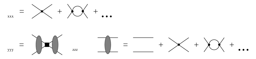
Figure 1: The leading and subleading contributions to the S–wave $T$–matrix in the case of unnaturally large scattering length. Solid dots (filled rectangles) refer to contact vertices without (with two) derivatives. Lines represent the nucleon propagators.

The leading term $T_{-1}$ results from summing an infinite chain of bubble diagrams with the lowest–order vertices. The corrections are given by perturbative insertions of higher–order interactions dressed to all orders by the leading vertices. Matching the resulting $T$–matrix with the one in Eq. (2.2) one finds at NLO:

$$C_{0}=\frac{4\pi}{m}\;\frac{1}{a^{-1}-\mu}\,,\mbox{\hskip 56.9055pt}C_{2}=\frac{4\pi}{m}\;\frac{1}{(a^{-1}-\mu)^{2}}\frac{r_{0}}{2}\,.$$ (2.36)

Notice that since $\mu\sim k$ and $a^{-1}\ll\mu$, the LECs $C_{0,2}$ scale as $C_{0}\sim 1/k$ and $C_{2}\sim 1/k^{2}$. More generally, a LEC $C_{2n}$ accompanying a vertex with $2n$ derivatives can be shown to scale as $C_{2n}\sim 1/k^{n+1}$ [75, 76]. This has to be contrasted with the scaling $C_{2n}\sim k^{0}$ in the case of a natural scattering length, cf. Eq. (2.33). Notice further that the LECs $C_{0,2}$ take very large values in the MS scheme (i.e. for $\mu=0$) which destroys the manifest power counting [75, 76].

The three–nucleon problem within pionless EFT has attracted a lot of scientific interest during the past few years, see e.g. [80, 81, 82, 83, 84, 85, 86, 87]. The ultimate question is to what extent the low–energy behavior of the 2N system constrains the properties of the three–nucleon (3N) system. Here, it is particularly interesting that one can identify universal properties of systems, where the scattering length in the two–body system is large. This situation is not only realized in the NN system, but also for ⁴He atoms and atomic systems close to a Feshbach resonance, see [88] for more details. The integral equation for the $T$–matrix describing nucleon–dimeron scattering and including the leading three–nucleon force is schematically depicted in Fig. 2.

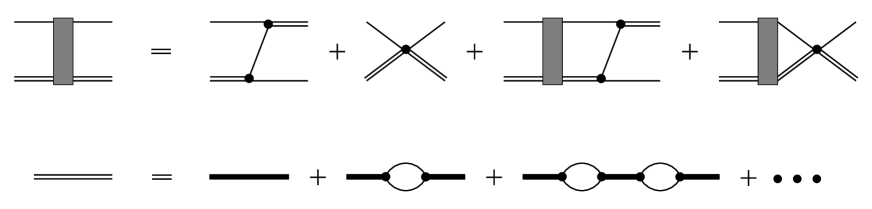
Figure 2: The first line is the graphical representation of the integral equation describing nucleon–dimeron scattering. The second line shows the dressed dimeron propagator. Double (bold) lines correspond to the dressed (bare) propagator of the dimeron. Shaded rectangles refer to the 3N $T$–matrix. For remaining notation see Fig. 1.

For simplicity, we here discuss the case of three interacting bosons, which gathers the main aspects of the problem. For the state with total orbital angular momentum $L=0$, the integral equation takes the following form in the three–body CMS:

$$T(k,p;\,E)=\frac{16}{3a}M(k,p;\,E)+\frac{4}{\pi}\int_{0}^{\Lambda}dq\,q^{2}\,T(k,q;\,E)\,\frac{1}{-a^{-1}+\sqrt{3q^{2}/4-mE-i\epsilon}}\,M(q,p;\,E)\,,$$ (2.37)

where the inhomogeneous term reads

$$M(k,p;\,E)=\frac{1}{2kp}\ln\left(\frac{k^{2}+kp+p^{2}-mE}{k^{2}-kp+p^{2}-mE}\right)+\frac{H(\Lambda)}{\Lambda^{2}}\,.$$ (2.38)

Here $a$ ($H$) is the two–body scattering length (the strength of the three–body force), $k\equiv|\vec{k}{}|$ ($p\equiv|\vec{p}\,|$) is the magnitude of the dimeron incoming (outgoing) momenta and $E=\frac{3k^{2}}{4m}-\gamma$ is the total energy in the incoming state with $\gamma\simeq(ma^{2})^{-1}$ being the two–body binding energy. The incoming and outgoing bosons are taken on the energy shell. The on–shell point corresponds to $k=p$ and the phase shift can be obtained via

$$\frac{1}{k\cot\delta-ik}=T(k,k;\,E)\,.$$ (2.39)

For $H=0$, $\Lambda\to\infty$, Eq. (2.37) has been first derived by Skorniakov and Ter-Martirosian [89]. It is well known that Eq. (2.37) has no unique solution in this limit [90]. The regularized equation has a unique solution for any given (finite) value of the ultraviolet cut–off $\Lambda$ but the amplitude in the absence of the three–body force shows an oscillatory behavior on $\Lambda$. Cut–off independence of the amplitude is restored by an appropriate “running” of $H(\Lambda)$ which turns out to be of a limit cycle type [81, 80]. Adjusting $H(\Lambda)$ to a single three–body observable for large enough $\Lambda$ (or even in the limit $\Lambda\to\infty$) allows to determine all other low–energy properties of the three–body system. Alternatively, this can also be achieved by choosing $H=0$, tuning $\Lambda$ to reproduce a three–body data point and using the same cut–off to calculate other observables [91]. It has also been conjectured that the behavior of the physical amplitude at asymptotically large momenta has to satisfy certain constraints which might be used to extract a unique solution of Eq. (2.37) in the case $H=0$ and $\Lambda\to\infty$ [92, 85].

The 3N problem can be considered as generalization of the bosonic case. For S–wave $Nd$ scattering in the spin–$3/2$ channel, the corresponding equation for the $T$–matrix has a unique solution for $H=0$ and $\Lambda\to\infty$ so that there is no need to include a 3N force. In the spin–$1/2$ channel two nucleons can form both spin–$1$ and spin–$0$ dimeron fields which leads to a pair of coupled integral equations for the $Nd$ $T$–matrix. Including the leading contact 3N force allows one to solve these equations in a cut–off independent way [82]. Thus, one needs a new parameter which is not determined in the 2N system in order to fix the (leading) low–energy behavior of the 3N system in this channel. Higher–order corrections to the amplitude including the ones due to 2N effective range terms can be included perturbatively [93, 84, 87]. Extension to 3N channels with different quantum numbers is straightforward [83]. For the current status of these applications see [94, 95, 96] and references therein. Universal low–energy properties of few–body systems with short–range interactions and large two–body scattering length are reviewed in [88], see also [97] for an early work on this subject. First results in the four–body sector within pionless EFT are presented in [98, 99]. Recently, this approach has also been applied to halo nuclei, see [96] for an overview. For more details on these and further topics including applications to a variety of electroweak processes in the 2N sector see the recent review articles [94, 95] and references therein.

2.3 Chiral EFT for few–nucleon systems

So far we have considered few–nucleon processes at very low momenta $k\ll M_{\pi}$ which can be well treated within pionless EFT. We now wish to go to higher momenta $k\sim M_{\pi}$ where the inclusion of explicit pions is mandatory. The interaction between pions and nucleons is governed by the spontaneously broken approximate chiral symmetry of QCD as explained in section 2.1. One would, therefore, like to have an approach which utilizes both resummation of certain classes of Feynman diagrams in order to describe the nonperturbative features of few–nucleon systems as well as chiral expansion familiar from the single–nucleon sector. While the leading NN contact interaction has to be resummed to all orders at least in the case of an unnaturally large scattering length, it is not clear a priori whether the interaction resulting from the exchange of pions between the nucleons is weak enough to be treated perturbatively. We will now outline two basic EFT approaches with explicit pions to few–nucleon systems: the one due to Kaplan, Savage and Wise (KSW) [75, 76] which treats pion exchange in perturbation theory, and the other one due to Weinberg [3, 4] based on its nonperturbative treatment. For yet another scheme see [100].

The KSW formalism represents a straightforward generalization of the pionless EFT approach for the case of large scattering length discussed in section 2.2 to perturbatively include diagrams with exchange of one or more pions. The scaling of the contact interactions is assumed to be the same as in pionless EFT (provided one uses DR with PDS or an equivalent scheme to regularize divergent loop integrals). For $k\sim M_{\pi}\sim a^{-1}$, the leading–order S–wave amplitude $T_{-1}$ is still given by the diagrams shown in the first line of Fig. 1. The first correction $T_{0}$ arises from perturbative insertions of subleading contact interactions (i.e. the ones with two derivatives and $\propto M_{\pi}^{2}$) and one–pion exchange (1PE) dressed to all orders by the leading contact interactions, see Fig. 3. The undressed static 1PE contribution corresponding to the second graph in Fig. 3 and based on the Lagrangian in Eq. (2.24) has the form

Figure 3: The first correction to the NN scattering amplitude in the KSW approach. Dashed lines refer to pions, solid rectangles denote insertions of vertices with two derivatives or proportional to $M_{\pi}^{2}$. For remaining notation see Fig. 1.

$$T_{0}^{\rm 1\pi,\,undressed}=-\frac{1}{4\pi}\left(\frac{g_{A}}{2F_{\pi}}\right)^{2}\,\mbox{\boldmath$\tau$}_{1}\cdot\mbox{\boldmath$\tau$}_{2}\,\frac{(\vec{\sigma}_{1}\cdot\vec{q}\,)(\vec{\sigma}_{2}\cdot\vec{q}\,)}{\vec{q}\,^{2}+M_{\pi}^{2}}\,,$$ (2.40)

where $\vec{q}=\vec{p}\,^{\prime}-\vec{p}$ is the nucleon momentum transfer and $\vec{\sigma}_{i}$ ($\mbox{\boldmath$\tau$}_{i}$) are spin (isospin) matrices of the nucleon $i$. The overall normalization of the $T$–matrix is consistent with Eq. (2.29). It is clear from Eq. (2.40) that this 1PE contribution as well as the contributions from the last two graphs in Fig. 3 are of the order $\mathcal{O}(k^{0})$. Notice that the coefficients of contact interactions with $2m$ derivatives and $\propto M_{\pi}^{2n-2m}$ are assumed to scale as $1/k^{n+1}$. Two–pion exchange (2PE) is suppressed compared to 1PE and starts to contribute at N²LO. At each order in the perturbative expansion, the amplitude is made independent on the renormalization scale by an appropriate running of the LECs $C_{i}$, $D_{i}$. As a nice feature, the KSW approach allows to derive analytic expressions for the scattering amplitude. In order to conclude on the usefulness of the KSW expansion with perturbative pions, it is crucial to understand the scale at which it fails. While in the single–nucleon sector, this scale is associated with the chiral symmetry breaking scale, $\Lambda_{\chi}\sim M_{\rho}\sim 4\pi F_{\pi}\sim 1$ GeV, the chiral expansion in the NN sector was found to entail the new scale $\Lambda_{NN}$ associated with the iterated 1PE contributions. Estimations based on dimensional analysis yield $\Lambda_{NN}=16\pi F_{\pi}^{2}/(g_{A}^{2}m)\sim 300$ MeV [75, 76]. In [95], an even more conservative result was obtained: $\Lambda_{NN}=4\pi F_{\pi}^{2}/(g_{A}^{2}m)\sim 70$ MeV. The small estimated values of $\Lambda_{NN}$ already indicate that the expansion based on perturbative pions might converge poorly. Clearly, dimensional analysis only provides a fairly rough estimation for the scale $\Lambda_{NN}$. The convergence of the KSW expansion can ultimately be only tested in concrete calculations. The 2N system has been analyzed at N²LO in [101]. While the results for the ${}^{1}S_{0}$ and some other partial waves including spin–singlet channels were found to be in reasonable agreement with the Nijmegen partial–wave analysis (PWA), large corrections show up in spin–triplet channels already at momenta $\sim 100$ MeV and lead to strong disagreements with the data. This is exemplified in Fig. 4. The perturbative inclusion of the pion–exchange contributions does not allow to increase the region of validity of the EFT compared to the pionless theory. The failure of the KSW approach in the spin–triplet channels was associated in [101] with the iteration of the tensor part of the 1PE potential. Further evidence of the poor convergence of the KSW expansion with perturbative pions was given by Cohen and Hansen [102, 103] who obtained predictions for the effective range and shape coefficients in the effective range expansion at lowest nontrivial order. These coefficients are sensitive to pion dynamics and were found to be poorly described, which indicates that the chiral expansion is not converging. More details on the KSW approach with explicit pions and its applications in the two– and three–nucleon sectors can be found in [94, 95] and references therein. For further discussion on the role of the pion–exchange contributions see [104, 105, 106, 107].

Figure 4: The NN ${}^{3}S_{1}$ phase shift $\bar{\delta}_{0}$ versus CMS momentum $p$. The solid line is the Nijmegen multi–energy fit [108, 109], the long dashed line is the LO EFT result, the short dashed line is the NLO result, and the dotted line is the N²LO result. The dash–dotted line shows the result of including a higher–order contact interaction. Figure courtesy of Ian W. Stewart.

A suitable way of including the pion–exchange contributions nonperturbatively was proposed in the seminal work of Weinberg [3, 4] which preceded the development of the KSW approach and caused a flurry of activities to apply EFT in the few–nucleon sector. Weinberg’s original arguments are formulated in terms of “old–fashioned” time–ordered perturbation theory, see e.g. [110], which is an appropriate tool since we are dealing with nonrelativistic nucleons. Consider the $S$–matrix for few–nucleon scattering

$$S_{\alpha\beta}=\delta(\alpha-\beta)-2\pi i\delta(E_{\alpha}-E_{\beta})T_{\alpha\beta}\,,$$ (2.41)

where $\alpha$ and $\beta$ denote the final and initial few–nucleon states and $E_{\alpha}$, $E_{\beta}$ are the corresponding energies. The $T$–matrix can be evaluated in “old–fashioned” time–ordered perturbation theory via

$$T_{\alpha\beta}=(H_{I})_{\alpha\beta}+\sum_{a}\frac{(H_{I})_{\alpha a}(H_{I})_{a\beta}}{E_{\beta}-E_{a}+i\epsilon}+\sum_{ab}\frac{(H_{I})_{\alpha a}(H_{I})_{ab}(H_{I})_{b\beta}}{(E_{\beta}-E_{a}+i\epsilon)(E_{\beta}-E_{b}+i\epsilon)}+\ldots\,,$$ (2.42)

where $H_{I}$ is the interaction Hamiltonian corresponding to the effective Lagrangian for pions and nucleons. Here, we use Latin letters for intermediate states, which, in general, may contain any number of pions, in order to distinguish them from purely nucleonic states denoted by Greek letters. We remind the reader that no nucleon–antinucleon pairs can be created or destroyed due to the nonrelativistic treatment of the nucleons. Consequently, all states contain the same number of nucleons. It is useful to represent various contributions to the scattering amplitude in terms of time–ordered diagrams. For example, the Feynman box diagram for NN scattering via $2\pi$–exchange can be expressed as a sum of six time–ordered graphs, see Fig. 5, which correspond to the following term in Eq. (2.42):

$$T_{\alpha\beta}^{2\pi}=\sum_{abc}\frac{(H_{\pi NN})_{\alpha a}(H_{\pi NN})_{ab}(H_{\pi NN})_{bc}(H_{\pi NN})_{c\beta}}{(E_{\beta}-E_{a}+i\epsilon)(E_{\beta}-E_{b}+i\epsilon)(E_{\beta}-E_{c}+i\epsilon)}\,,$$ (2.43)

where $H_{\pi NN}$ denotes the $\pi NN$ vertex. It is easy to see that the contributions of diagrams (d–g) are enhanced due to the presence of the small (of the order $Q^{2}/m$) energy denominator associated with the purely nucleonic intermediate state $|b\rangle$ which in the CMS takes the form:

$$\frac{1}{E_{\beta}-E_{b}+i\epsilon}=\frac{1}{\vec{p}_{\beta}^{\,2}/m-\vec{p}_{b}^{\,2}/m+i\epsilon}\,.$$ (2.44)

Notice that the energy denominators corresponding to the $\pi NN$ states $|a\rangle$ and $|c\rangle$ are of the order $M_{\pi}\sim Q$. According to Weinberg, the failure of perturbation theory in the few–nucleon sector is caused by the enhanced contribution of reducible diagrams, i.e. those ones which contain purely nucleonic intermediate states. To see how this difficulty can be dealt with, it is useful to rearrange the expansion in Eq. (2.42) and to write it in the form of the Lippmann–Schwinger equation

$$T_{\alpha\beta}=(V_{\rm eff})_{\alpha\beta}+\sum_{\gamma}\frac{(V_{\rm eff})_{\alpha\gamma}T_{\gamma\beta}}{E_{\beta}-E_{\gamma}+i\epsilon}\,,$$ (2.45)

with the effective potential $(V_{\rm eff})_{\alpha\beta}$ defined as a sum of all possible irreducible diagrams (i.e. the ones which do not contain purely nucleonic intermediate states):

$$(V_{\rm eff})_{\alpha\beta}=(H_{I})_{\alpha\beta}+\sum_{\tilde{a}}\frac{(H_{I})_{\alpha\tilde{a}}(H_{I})_{\tilde{a}\beta}}{E_{\beta}-E_{\tilde{a}}+i\epsilon}+\sum_{\tilde{a}\tilde{b}}\frac{(H_{I})_{\alpha\tilde{a}}(H_{I})_{\tilde{a}\tilde{b}}(H_{I})_{\tilde{b}\beta}}{(E_{\beta}-E_{\tilde{a}}+i\epsilon)(E_{\beta}-E_{\tilde{b}}+i\epsilon)}+\ldots\,.$$ (2.46)

Here, the states $|\tilde{a}\rangle$, $|\tilde{b}\rangle$ contain at least one pion. The effective potential in Eq. (2.46) does not contain small energy denominators and can be obtained within the low–momentum expansion following the usual procedure of CHPT. The contribution of a given irreducible time–ordered diagram can be shown to be of the order $(Q/\Lambda)^{\nu}$ [3, 4] with $\Lambda$ being the scale which enters the values of the renormalized LECs, where

$$\nu=-2+2N+2(L-C)+\sum_{i}V_{i}\Delta_{i}\,,\quad\mbox{where}\quad\Delta_{i}=d_{i}+\frac{1}{2}n_{i}-2\,.$$ (2.47)

Here $N$, $L$, $C$ and $V_{i}$ are the numbers of nucleons, loops, separately connected pieces and vertices of type $i$, respectively. The quantity $\Delta_{i}$ gives the chiral dimension of a vertex of type $i$.

Figure 5: Two–pion exchange: Feynman diagram (a) and the corresponding time–ordered graphs (b–g). Solid (dashed) lines correspond to nucleons (pions).

Further, $d_{i}$ denotes the number of derivatives or $M_{\pi}$ insertions and $n_{i}$ is the number of nucleon lines at the vertex $i$. Notice that eq. (2.47) is modified compared to the one given in Refs. [3, 4, 113] in order to account for the proper normalization of the $N$–nucleon states. Chiral symmetry guarantees that $\Delta_{i}\geq 0$. Consequently, the chiral order $\nu$ is bounded from below and for any given $\nu$ only a finite number of diagrams needs to be taken into account. Notice that Eq. (2.47) supports a rather natural view of nuclear dynamics, in which nucleons interact mainly via 2N forces while many–body forces provide small corrections. After the potential is obtained at a given order in the chiral expansion, few–nucleon observables can be calculated by solving the Lippmann–Schwinger equation (2.45), which leads to a nonperturbative resummation of the contributions resulting from reducible diagrams. It is easy to see from Eq. (2.47) that the leading–order ($\nu=0$) potential results from contact interactions without derivatives and the $1\pi$–exchange. This has to be contrasted with the KSW approach, where the exchange of pions is suppressed compared to the lowest–order contact terms. It should be understood that the power counting rules in Eq. (2.47) apply to renormalized matrix elements. After removing the ultraviolet divergences by a redefinition of the LECs in the effective Lagrangian, the remaining integrals are effectively cut off at momenta of the order of the soft scale $Q$. The power counting described above is based on an assumption, sometimes referred to as the naturalness assumption, that a renormalized coupling constant $C$ of dimension [mass]^-n can be written in terms of a dimensionless coefficient $c\sim\mathcal{O}(1)$ as $C=c\Lambda^{-n}$. Clearly, higher–dimensional terms in the amplitude are only suppressed if the hard scale $\Lambda$ that enters the values of the LECs is sufficiently large, i.e. if $Q\sim M_{\pi}\ll\Lambda$. The validity of the naturalness assumption can, at present, only be verified upon performing actual calculations.

The presence of shallow bound states in few–nucleon systems suggests that the perturbative (iterative) solution of Eq. (2.45) does not converge. As pointed out by Weinberg [3, 4], this requires for the nucleon mass to be counted as a much larger scale compared to the hard scale $\Lambda$. To see that consider the iteration of the leading order potential $V_{\rm eff}^{(0)}$ in the Lippmann–Schwinger equation (2.45) which, in operator form, can be written symbolically as

$$T=V_{\rm eff}^{(0)}+V_{\rm eff}^{(0)}\,G_{0}\,V_{\rm eff}^{(0)}+V_{\rm eff}^{(0)}\,G_{0}\,V_{\rm eff}^{(0)}\,G_{0}\,V_{\rm eff}^{(0)}+\ldots\,,$$ (2.48)

where $G_{0}$ is the free 2N resolvent operator. One can estimate the size of the leading–order potential by the size of the static $1\pi$–exchange potential leading to $V_{\rm eff}^{(0)}\sim 1/F_{\pi}^{2}$. Since each momentum integration in Eq. (2.48) gives an additional factor $Q^{3}/(4\pi)^{2}$ and $G_{0}\sim m/Q^{2}$, one finds that the $(n+1)$–th term in the above equation is suppressed compared to the first term by $(Qm/\Lambda^{2})^{n}$, where we used the estimation $\Lambda\sim 4\pi F_{\pi}$. The requirement that all terms in the right–hand side of Eq. (2.48) are of the same order in order, which justifies the necessity of the nonperturbative treatment and enables to describe the physics associated with the low–lying bound states, therefore leads to the following counting rule for the nucleon mass [3, 4, 119]:

$$\frac{Q}{m}\sim\frac{Q^{2}}{\Lambda^{2}}\,.$$ (2.49)

This counting rule will be adopted in the present work. Clearly, this estimation based on the naive dimensional analysis is fairly crude. A somewhat different estimation can be found in [95]. Notice that it is hardly possible in such an estimation to keep track of various numerical factors, even of the large factors such as $4\pi$. For example, the leading and subleading $2\pi$–exchange potentials, both arising from 1–loop diagrams, differ by a factor $4\pi$, see section 3.2.2. Fortunately, the particular way of counting the nucleon mass is not crucial from the practical point of view since it only determines the relative importance of the relativistic corrections to the nuclear force but does not affect the lowest–order potential and, therefore, also not the dominant contribution to the scattering amplitude. Finally, we stress that Weinberg’s power counting does not explain the unnaturally large values of the NN S–wave scattering lengths or, equivalently, the unnaturally small binding energies of the deuteron and the virtual bound state in the ${}^{1}S_{0}$ channel. This has to be achieved via an appropriate fine tuning of the lowest–order contact interactions.

To summarize, the “Weinberg program” for describing the low–energy dynamics of the few–nucleon systems proceeds in two basic steps which will be discussed in detail in the next sections of this review. First, the few–nucleon potential has to be derived from the effective Lagrangian for pions and nucleons using the framework of chiral perturbation theory. Secondly, the corresponding dynamical equations with the resulting potential as an input have to be solved.

3 Nuclear forces in chiral effective field theory

In the previous section we have introduced the basic concept of the Weinberg approach to few–nucleon systems. We will now discuss the structure of the nuclear force in the lowest orders in the chiral expansion based on the effective Lagrangian

$$\mathcal{L}^{(0)} = \frac{1}{2}\partial_{\mu}\mbox{\boldmath$\pi$}\cdot\partial^{\mu}\mbox{\boldmath$\pi$}-\frac{1}{2}M^{2}\mbox{\boldmath$\pi$}^{2}+N^{\dagger}\bigg{[}i\partial_{0}+\frac{g_{A}}{2F}\mbox{\boldmath$\tau$}\vec{\sigma}\cdot\vec{\nabla}\mbox{\boldmath$\pi$}-\frac{1}{4F^{2}}\mbox{\boldmath$\tau$}\cdot(\mbox{\boldmath$\pi$}\times\dot{\mbox{\boldmath$\pi$}})\bigg{]}N$$

$${}-\frac{1}{2}C_{S}(N^{\dagger}N)(N^{\dagger}N)-\frac{1}{2}C_{T}(N^{\dagger}\vec{\sigma}N)(N^{\dagger}\vec{\sigma}N)+\ldots\,,$$

$$\mathcal{L}^{(1)} = N^{\dagger}\bigg{[}4c_{1}M^{2}-\frac{2c_{1}}{F^{2}}M^{2}\mbox{\boldmath$\pi$}^{2}+\frac{c_{2}}{F^{2}}\dot{\mbox{\boldmath$\pi$}}^{2}+\frac{c_{3}}{F^{2}}(\partial_{\mu}\mbox{\boldmath$\pi$}\cdot\partial^{\mu}\mbox{\boldmath$\pi$})-\frac{c_{4}}{2F^{2}}\epsilon_{ijk}\,\epsilon_{abc}\,\sigma_{i}\tau_{a}(\nabla_{j}\,\pi_{b})(\nabla_{k}\,\pi_{c})\bigg{]}N$$ (3.1)

$${}-\frac{D}{4F}(N^{\dagger}N)(N^{\dagger}\vec{\sigma}\mbox{\boldmath$\tau$}N)\cdot\vec{\nabla}\mbox{\boldmath$\pi$}-\frac{1}{2}E\,(N^{\dagger}N)(N^{\dagger}\mbox{\boldmath$\tau$}N)\cdot(N^{\dagger}\mbox{\boldmath$\tau$}N)+\ldots\,,$$

where the superscripts denote the vertex dimension $\Delta_{i}$, see Eq. (2.47), $c_{i}$, $C_{S,T}$, $D$ and $E$ are LECs and ellipses refer to terms with more pion fields. Notice that the nucleon kinetic energy contribute, according to Eq. (2.49), to $\mathcal{L}^{(2)}$. The above terms determine the nuclear potential up to N²LO (with the exception of the NN contact terms at NLO) in the limit of exact isospin symmetry. More complete expressions for the Lagrangian including higher–order terms can be found e.g. in [64, 120, 121, 122, 123, 124, 125].

3.1 Nuclear potentials from field theory

The derivation of a potential from field theory is an intensively studied problem in nuclear physics. Historically, the important conceptual achievements in this field have been done in the fifties of the last century in the context of the so called meson field theory. The problem can be formulated in the following way: given a field theoretical Lagrangian for interacting mesons and nucleons, how can one reduce the (infinite dimensional) equation of motion for mesons and nucleons to an effective Schrödinger equation for nucleonic degrees of freedom, which can be solved by standard methods? It goes beyond the scope of this work to address the whole variety of different techniques which have been developed to construct effective interactions, see Ref. [126] for a comprehensive review. We will now briefly outline a few methods which have been used in the context of chiral EFT.

We begin with the approach developed by Tamm [127] and Dancoff [128] which in the following will be referred to as the Tamm–Dancoff method. Consider the time–independent Schrödinger equation

$$(H_{0}+H_{I})|\Psi\rangle=E|\Psi\rangle\,,$$ (3.2)

where $|\Psi\rangle$ denotes an eigenstate of the Hamiltonian $H$ with the eigenvalue $E$. One can divide the full Fock space in to the nucleonic subspace $|\phi\rangle$ and the complementary one $|\psi\rangle$ and rewrite the Schrödinger equation (3.2) as

$$\left(\begin{array}[]{cc}\eta H\eta&\eta H\lambda\\ \lambda H\eta&\lambda H\lambda\end{array}\right)\left(\begin{array}[]{c}|\phi\rangle\\ |\psi\rangle\end{array}\right)=E\left(\begin{array}[]{c}|\phi\rangle\\ |\psi\rangle\end{array}\right)~{},\quad\,$$ (3.3)

where we introduced the projection operators $\eta$ and $\lambda$ such that $|\phi\rangle=\eta|\Psi\rangle$, $|\psi\rangle=\lambda|\Psi\rangle$. Expressing the state $|\psi\rangle$ from the second line of the matrix equation (3.3) as

$$|\psi\rangle=\frac{1}{E-\lambda H\lambda}H|\phi\rangle~{},$$ (3.4)

and substituting this in to the first line one obtains the Schrödinger–like equation for the projected state $|\phi\rangle$:

$$\left(H_{0}+V_{{\rm eff}}^{\rm TD}(E)\right)|\phi\rangle=E|\phi\rangle\,,$$ (3.5)

with an effective potential $V_{\rm eff}(E)$ given by

$$V_{\rm eff}^{\rm TD}(E)=\eta H_{I}\eta+\eta H_{I}\lambda\frac{1}{E-\lambda H\lambda}\lambda H_{I}\eta\,\,.$$ (3.6)

It is easy to see that the above definition of the effective potential is identical with the one given in Eq. (2.46) in the context of “old–fashioned” time–ordered perturbation theory. We stress that in order to evaluate $V_{\rm eff}^{\rm TD}(E)$ one usually has to rely on perturbation theory. For example, for the Yukawa theory with $H_{I}=gH_{1}$, the effective potential $V_{\rm eff}^{\rm TD}(E)$ up to the fourth order in the coupling constant $g$ is given by

$$V_{\rm eff}^{\rm TD}(E)=-\eta^{\prime}\bigg{[}g^{2}H_{1}\frac{\lambda^{1}}{H_{0}-E}H_{1}+g^{4}H_{1}\frac{\lambda^{1}}{H_{0}-E}H_{1}\frac{\lambda^{2}}{H_{0}-E}H_{1}\frac{\lambda^{1}}{H_{0}-E}H_{1}+\mathcal{O}(g^{6})\bigg{]}\eta\,,$$ (3.7)

where the superscripts of $\lambda$ refer to the number of mesons in the corresponding state. It is important to realize that the effective potential $V_{{\rm eff}}(E)$ in this scheme depends explicitly on the energy, which makes it inconvenient for practical applications. In addition, the projected nucleon states $|\phi\rangle$ have a normalization different from the states $|\Psi\rangle$ we have started from, which are assumed to span a complete and orthonormal set in the whole Fock space:

$$\langle\phi_{i}|\phi_{j}\rangle=\langle\Psi_{i}|\Psi_{j}\rangle-\langle\psi_{i}|\psi_{j}\rangle=\delta_{ij}-\langle\phi_{i}|H_{I}\lambda\left(\frac{1}{E-\lambda H\lambda}\right)^{2}\lambda H_{I}|\phi_{j}\rangle~{}.$$ (3.8)

Note that the components $\psi_{i}$ in this equation do, in general, not vanish.

The above mentioned deficiencies are naturally avoided in the method of unitary transformation [129], see also [130]. In this approach, the decoupling of the $\eta$– and $\lambda$–subspaces of the Fock space is achieved via a unitary transformation $U$

$$\tilde{H}\equiv U^{\dagger}HU=\left(\begin{array}[]{cc}\eta\tilde{H}\eta&0\\ 0&\lambda\tilde{H}\lambda\end{array}\right)\,.$$ (3.9)

Following Okubo [129], the unitary operator $U$ can be parametrized as

$$U=\left(\begin{array}[]{cc}\eta(1+A^{\dagger}A)^{-1/2}&-A^{\dagger}(1+AA^{\dagger})^{-1/2}\\ A(1+A^{\dagger}A)^{-1/2}&\lambda(1+AA^{\dagger})^{-1/2}\end{array}\right)~{},$$ (3.10)

with the operator $A=\lambda A\eta$. The operator $A$ has to satisfy the decoupling equation

$$\lambda\left(H-\left[A,\;H\right]-AHA\right)\eta=0$$ (3.11)

in order for the transformed Hamiltonian $\tilde{H}$ to be of block–diagonal form. The effective $\eta$–space potential $\tilde{V}_{\rm eff}^{\rm UT}$ can be expressed in terms of the operator $A$ as:

$$\tilde{V}_{\rm eff}^{\rm UT}=\eta(\tilde{H}-H_{0})=\eta\bigg{[}(1+A^{\dagger}A)^{-1/2}(H+A^{\dagger}H+HA+A^{\dagger}HA)(1+A^{\dagger}A)^{-1/2}-H_{0}\bigg{]}\eta~{}.$$ (3.12)

For the previously considered case of the Yukawa theory, the operator $A$ and the effective potential $V_{\rm eff}^{\rm UT}$ can be obtained within the expansion in powers of the coupling constant $g$, which leads to:

$$V_{\rm eff}^{\rm UT} = -g^{2}\,\eta^{\prime}\Bigg{[}\frac{1}{2}H_{1}\frac{\lambda^{1}}{H_{0}-E_{\eta}}H_{1}+\mbox{h.~{}c.}\Bigg{]}\eta-g^{4}\,\eta^{\prime}\Bigg{[}\frac{1}{2}H_{1}\frac{\lambda^{1}}{(H_{0}-E_{\eta})}H_{1}\,\frac{\lambda^{2}}{(H_{0}-E_{\eta})}\,H_{1}\frac{\lambda^{1}}{(H_{0}-E_{\eta})}H_{1}$$ (3.13)

$${}-\frac{1}{2}H_{1}\frac{\lambda^{1}}{(H_{0}-E_{\eta^{\prime}})}H_{1}\,\tilde{\eta}\,H_{1}\frac{\lambda^{1}}{(H_{0}-E_{\tilde{\eta}})(H_{0}-E_{\eta^{\prime}})}H_{1}$$

$${}+\frac{1}{8}H_{1}\frac{\lambda^{1}}{(H_{0}-E_{\eta^{\prime}})}H_{1}\,\tilde{\eta}\,H_{1}\frac{\lambda^{1}}{(H_{0}-E_{\tilde{\eta}})(H_{0}-E_{\eta})}H_{1}$$

$${}-\frac{1}{8}H_{1}\frac{\lambda^{1}}{(H_{0}-E_{\eta^{\prime}})(H_{0}-E_{\tilde{\eta}})}H_{1}\,\tilde{\eta}\,H_{1}\frac{\lambda^{1}}{(H_{0}-E_{\tilde{\eta}})}H_{1}+\mbox{h.~{}c.}\Bigg{]}\eta+\mathcal{O}(g^{6})\,.$$

In contrast to $V_{\rm eff}^{\rm TD}$ given in Eq. (3.7), $V_{\rm eff}^{\rm UT}$ does not depend on the energy $E$. Another difference to the Tamm–Dancoff method is given by the presence of terms with the projection operator $\tilde{\eta}$ which give rise to purely nucleonic intermediate states. These terms are needed to ensure the proper normalization of the few–nucleon states. It should be understood that, in spite of the presence of the purely nucleonic intermediate states, such terms are not generated through the iteration of the dynamical equation and are thus not reducible in the language of section 2.3. Since all energy denominators in Eq. (3.13) correspond to intermediate states with at least one pion, there is no enhancement by large factors of $m/Q$, which is typical for reducible contributions.

The two methods of deriving effective nuclear potentials are quite general and can, in principle, be applied to any field theoretical meson–nucleon Lagrangian. In the weak coupling case, the potential can be obtained straightforwardly via the expansion in powers of the corresponding coupling constant(s). Generalization to the effective chiral Lagrangian requires the expansion in powers of the coupling constants to be replaced by the chiral expansion in powers of $Q/\Lambda$. For practical applications, it is helpful to use time–ordered diagrams to visualize the contributions to the potential. In “old–fashioned” perturbation theory or, equivalently, the Tamm–Dancoff approach, only irreducible diagrams are allowed. Their importance is determined by the power counting in Eq. (2.47) and the explicit contributions can be found using Eq. (3.6). In the method of unitary transformation one can draw both irreducible and reducible graphs, whose importance is still given by Eq. (2.47). Notice that these graphs have a different meaning from the time–ordered ones arising in the context of “old–fashioned” perturbation theory and will only be used to visualize the topology associated with a given sequence of vertices. The structure of the operators contributing to the potential can, in general, not be guessed by looking at a given diagram and has to be determined by solving the decoupling equation (3.11) for the operator $A$ and using Eq. (3.12). This is discussed in detail in Refs. [131, 132], where it is also demonstrated how to derive the effective potential from the effective chiral Lagrangian at any given order $\nu$ in the low–momentum expansion using the method of unitary transformation, see also [133] for a different but closely related scheme. The explicit expressions for the operators contributing to the potential in the few lowest orders can be found in these references. For issues related to renormalization within the method of unitary transformation see Ref. [134]. Another Hamiltonian approach, which is similar to the method of unitary transformation and is usually referred to as the dressed particle approach, is extensively discussed in Refs. [135, 136, 137, 138].

To illustrate how the above ideas work in practice, let us consider the contribution to the leading $2\pi$–exchange potential at order $\nu=2$ arising from diagram (a) in Fig. 5. The Hamilton operator $H^{(0)}$ describing the $\pi NN$ vertex of the lowest possible dimension, $\Delta_{i}=0$, corresponds to the last term in Eq. (2.17). In “old–fashioned” perturbation theory, the potential arises from diagrams (b) and (c) in Fig. 5 and can be obtained evaluating the appropriate matrix elements of the operator

$$V^{\rm TD}_{2\pi}=-\eta H^{(0)}\frac{\lambda^{1}}{\omega}H^{(0)}\frac{\lambda^{2}}{\omega_{1}+\omega_{2}}H^{(0)}\frac{\lambda^{1}}{\omega}H^{(0)}\eta\,,$$ (3.14)

where $\omega_{i}=\sqrt{\vec{k}\,^{2}+M_{\pi}^{2}}$ denotes the energy of a pion with the momentum $\vec{k}$. Notice that at the order considered, it is sufficient to treat nucleons as static sources. Explicit evaluation of Eq. (3.14) yields the following result in the CMS [119]:

$$V^{\rm TD}_{2\pi} = -\frac{g_{A}^{4}}{4(2F_{\pi})^{4}}\,\int\,\frac{d^{3}l}{(2\pi)^{3}}\,\frac{1}{\omega_{+}^{3}\omega_{-}}\Bigg{\{}\left(\frac{3}{\omega_{-}}+\frac{2\mbox{\boldmath$\tau$}_{1}\cdot\mbox{\boldmath$\tau$}_{2}}{\omega_{+}+\omega_{-}}\right)\left({\vec{l}\,}^{2}-{\vec{q}\,}^{2}\right)^{2}$$

$$\mbox{\hskip 71.13188pt}+4\left(\frac{3}{\omega_{+}+\omega_{-}}+\frac{2\mbox{\boldmath$\tau$}_{1}\cdot\mbox{\boldmath$\tau$}_{2}}{\omega_{-}}\right)(\vec{\sigma}_{2}\cdot[\vec{q}\times\vec{l}\,])(\vec{\sigma}_{1}\cdot[\vec{q}\times\vec{l}\,])\Bigg{\}}\;,$$

with $\omega_{\pm}\equiv\sqrt{(\vec{q}\pm\vec{l}\,)^{2}+4M_{\pi}^{2}}$ and $\vec{q}$ being the nucleon momentum transfer. In the method of unitary transformation, the potential is due to diagrams (b–g) in Fig. 5 and is given by:

$$V^{\rm UT}_{2\pi}=V^{\rm TD}_{2\pi}+\frac{1}{2}\eta H^{(0)}\frac{\lambda^{1}}{\omega^{2}}H^{(0)}\eta H^{(0)}\frac{\lambda^{1}}{\omega}H^{(0)}\eta+\frac{1}{2}\eta H^{(0)}\frac{\lambda^{1}}{\omega}H^{(0)}\eta H^{(0)}\frac{\lambda^{1}}{\omega^{2}}H^{(0)}\eta\,.$$ (3.16)

The first term on the right–hand side of the above equation, $V^{\rm TD}_{2\pi}$, gives the contribution of the irreducible graphs (b) and (c) which, for static nucleons, is the same as in the previously considered case. The contribution of reducible diagrams (d–g) is given by the last two terms in the above equation. The resulting potential has the form [139]:

$$V^{\rm UT}_{2\pi}=-\frac{g_{A}^{4}}{2(2F_{\pi})^{4}}\,\int\,\frac{d^{3}l}{(2\pi)^{3}}\,\frac{\omega_{+}^{2}+\omega_{+}\omega_{-}+\omega_{-}^{2}}{\omega_{+}^{3}\omega_{-}^{3}(\omega_{+}+\omega_{-})}\Bigg{\{}\mbox{\boldmath$\tau$}_{1}\cdot\mbox{\boldmath$\tau$}_{2}\left({\vec{l}\,}^{2}-{\vec{q}\,}^{2}\right)^{2}+6(\vec{\sigma}_{2}\cdot[\vec{q}\times\vec{l}\,])(\vec{\sigma}_{1}\cdot[\vec{q}\times\vec{l}\,])\Bigg{\}}\;.$$

Notice that the isoscalar central and isovector tensor components in Eq. (3.1) cancel in the method of unitary transformation against the contributions from reducible diagrams. We will discuss the chiral $2\pi$–exchange potential in more detail in section 3.2.2.

Before closing this section, let us mention two other methods to derive energy–independent potentials used in the context of chiral EFT. Historically, energy–independent expressions for the chiral $2\pi$–exchange potential at order $\nu=2$ were first obtained by Friar and Coon [140] using the method described in [141]. Yet another approach was applied e.g. in Refs. [142, 143, 144, 145] to study chiral $2\pi$– and $3\pi$–exchange forces, in which the potential is determined through matching to the $S$–matrix.

Last but not least, one should always keep in mind that, in contrast to the on–shell scattering amplitude, nuclear potentials themselves are not experimentally observable and can always be modified via a unitary transformation, see e.g. [146] for some explicit examples. This non–uniqueness of the nuclear forces should, of course, not be considered as a conceptual problem. A similar sort of non–uniqueness at the level of the Lagrangian is well known in quantum field theory, where one has the freedom to perform nonlinear field redefinitions. Notice that unitary transformations will, in general, affect not only few–nucleon forces but also the corresponding nuclear current operators. It is, therefore, important to have a consistent (in the above mentioned sense) formulation for 2N, 3N, $\ldots$, forces and current operators. Such a consistent formulation is provided by the chiral EFT framework.

3.2 Two–nucleon force

The chiral NN force has the general form

$$V_{\rm 2N}=V_{\pi}+V_{\rm cont}\,,$$ (3.17)

where $V_{\rm cont}$ denotes the short–range terms represented by $NN$ contact interactions and $V_{\pi}$ corresponds to the long–range part associated with the pion–exchange contributions Both $V_{\pi}$ and $V_{\rm cont}$ are determined within the low–momentum expansion as will be discussed in the next sections.

3.2.1 Regularization of the pion–exchange contributions

Let us now take a closer look at the pion–exchange contributions. The explicit form of the corresponding non–polynomial functions of momenta depends, to some extent, on the way one regularizes the corresponding loop integrals. Consider, for example, the isoscalar central part of the 2PE potential at order $\nu=3$ which results from the triangle diagrams and is given by

$$V_{\rm C}(q)=\frac{3g_{A}^{2}}{16F_{\pi}^{4}}\int\,\frac{d^{3}l}{(2\pi)^{3}}\frac{l^{2}-q^{2}}{\omega_{-}^{2}\omega_{+}^{2}}\left(8c_{1}M_{\pi}^{2}+c_{3}(l^{2}-q^{2})\right)\,,$$ (3.18)

where $q\equiv|\vec{q}\,|$, $l\equiv|\vec{l}\,|$ and $c_{i}$ are the corresponding LECs. The integral is cubically divergent and needs to be regularized. Applying dimensional regularization one finds:

$$V_{\rm C}(q)=-\frac{3g_{A}^{2}}{16\pi F_{\pi}^{4}}\left(2M_{\pi}^{2}(2c_{1}-c_{3})-c_{3}q^{2}\right)(2M_{\pi}^{2}+q^{2})\,A(q)\;,\quad\quad\quad A(q)=\frac{1}{2q}\arctan\frac{q}{2M_{\pi}}\,.$$ (3.19)

Here, we do not show polynomial terms of the kind $\alpha+\beta q^{2}$ which contribute to $V_{\rm cont}$. It is instructive to express the potential using the spectral function representation:

$$V_{\rm C}(q)=\frac{2q^{4}}{\pi}\int_{2M_{\pi}}^{\infty}d\mu\,\frac{1}{\mu^{3}}\,\frac{\rho(\mu)}{\mu^{2}+q^{2}},$$ (3.20)

where the spectral function $\rho(\mu)$ can be obtained from $V_{\rm C}(q)$ in Eq. (3.19) via

$$\rho(\mu)=\Im\left[V_{\rm C}(0^{+}-i\mu)\right]=-\frac{3g_{A}^{2}}{64F_{\pi}^{4}}\left(2M_{\pi}^{2}(2c_{1}-c_{3})+c_{3}\mu^{2}\right)(2M_{\pi}^{2}-\mu^{2})\frac{1}{\mu}\theta(\mu-2M_{\pi})\,.$$ (3.21)

In Eq. (3.20), the twice subtracted dispersion integral is given which is needed in order to account for the large–$\mu$ behavior of $\rho(\mu)$. Eq. (3.20) shows that the 2PE potential resulting from Eq. (3.18) upon applying DR contains explicitly the short–range contributions associated with the integration over large values of $\mu$. These short–range contributions to the potential are an artifact of the chosen regularization procedure (i.e. DR). They are model dependent and cannot be predicted in the chiral EFT framework since the chiral expansion for the spectral function $\rho(\mu)$ is invalid for large values of $\mu$. Instead of keeping the spurious short–range physics in the 2PE potential, one can perform the spectral function integral only over the low–$\mu$ region, where chiral EFT is applicable. This can be achieved using the regularized spectral function

$$\rho(\mu)\rightarrow\rho^{\tilde{\Lambda}}(\mu)=\rho(\mu)\,\theta(\tilde{\Lambda}-\mu)\,,$$ (3.22)

with the reasonably chosen finite ultraviolet cut–off $\tilde{\Lambda}$ which prevents that the regularized 2PE potential $V_{\rm C}^{\tilde{\Lambda}}$ given by

$$V_{\rm C}^{\tilde{\Lambda}}=\frac{2q^{4}}{\pi}\int_{2M_{\pi}}^{\infty}d\mu\,\frac{1}{\mu^{3}}\,\frac{\rho^{\tilde{\Lambda}}(\mu)}{\mu^{2}+q^{2}}=-\frac{3g_{A}^{2}}{16\pi F_{\pi}^{4}}\left(2M_{\pi}^{2}(2c_{1}-c_{3})-c_{3}q^{2}\right)(2M_{\pi}^{2}+q^{2})\,A^{\tilde{\Lambda}}(q)+\ldots\,,$$ (3.23)

with the ellipses referring to polynomial (in $q^{2}$) terms has components with the range $r<\tilde{\Lambda}^{-1}$. In the above equation, the regularized loop function $A^{\tilde{\Lambda}}(q)$ turns out to be

$$A^{\tilde{\Lambda}}(q)=\theta(\tilde{\Lambda}-2M_{\pi})\frac{1}{2q}\arctan\frac{q(\tilde{\Lambda}-2M_{\pi})}{q^{2}+2\tilde{\Lambda}M_{\pi}}\,.$$ (3.24)

In what follows, we will refer to the above described regularization scheme, which has been introduced in [147], as to spectral function regularization (SFR).

What is the relation between the DR and SFR potentials in Eqs. (3.19) and (3.23)? To see that one can rewrite the spectral function integral in Eq. (3.20) as follows:

$$\frac{2q^{4}}{\pi}\int_{2M_{\pi}}^{\infty}d\mu\,\frac{1}{\mu^{3}}\,\frac{\rho(\mu)}{\mu^{2}+q^{2}} = \frac{2q^{4}}{\pi}\int_{2M_{\pi}}^{\tilde{\Lambda}}d\mu\,\frac{1}{\mu^{3}}\,\frac{\rho(\mu)}{\mu^{2}+q^{2}}+\frac{2q^{4}}{\pi}\int_{\tilde{\Lambda}}^{\infty}d\mu\,\frac{1}{\mu^{3}}\,\frac{\rho(\mu)}{\mu^{2}+q^{2}}$$ (3.25)

$$\stackrel{{\scriptstyle q<\tilde{\Lambda}}}{{\longrightarrow}} \frac{2q^{4}}{\pi}\int_{2M_{\pi}}^{\infty}d\mu\,\frac{1}{\mu^{3}}\,\frac{\rho^{\tilde{\Lambda}}(\mu)}{\mu^{2}+q^{2}}+\alpha q^{4}+\beta q^{6}+\ldots\,,$$

where

$$\alpha=\frac{2}{\pi}\int_{\tilde{\Lambda}}^{\infty}d\mu\,\frac{\rho(\mu)}{\mu^{5}}\,,\quad\quad\beta=-\frac{2}{\pi}\int_{\tilde{\Lambda}}^{\infty}d\mu\,\frac{\rho(\mu)}{\mu^{7}}\,,\quad\quad\ldots\,.$$ (3.26)

It is, therefore, obvious, that the DR and SFR potentials differ from each other by an infinite series of higher–order contact interactions. In fact, they might be viewed as two different conventions to define the non–polynomial part of the two– and more–pion exchange potential. DR corresponds to the convention, according to which the non–polynomial part includes components of arbitrarily short range which are strongly model–dependent. In contrast, the SFR approach uses the convention, according to which only the components with the range $r>\tilde{\Lambda}^{-1}$ are explicitly kept in the non–polynomial part of the potential while all shorter–range contributions are represented by the contact interactions. In general, for quickly converging expansions, both the DR and SFR methods are completely equivalent provided the ultraviolet cut–off $\tilde{\Lambda}$ is chosen to be large enough. For example, we will see in section 4.1.1, that both schemes lead to similar results for peripheral NN scattering at order $\nu=2$. If, however, the convergence for some well understood physical reason is slow and (some) observables become sensitive to higher–order counter terms, it is safer to avoid the spurious short–distance contributions kept in DR. In such a case, SFR is a preferable choice. An example of such a situation will be considered in section 4.1.1. Notice that a similar approach based on a finite momentum cut–off was used in [148, 149, 150] to deal with the slow convergence in the SU(3) baryon CHPT, see also [151] for a recent application to the chiral extrapolation of the lattice QCD results and [152, 153] for a discussion on cut–off schemes in CHPT.

It is also instructive to compare the DR and SFR potentials in configuration space. For $r>0$, the inverse Fourier–transform can be expressed in terms of the spectral function $\rho(\mu)$ via

$$V_{\rm C}(r)=\frac{1}{2\pi^{2}r}\int_{2M_{\pi}}^{\infty}d\mu\,\mu\,e^{-\mu r}\rho(\mu).$$ (3.27)

Substituting $\rho(\mu)$ from Eq. (3.21) in to Eq. (3.27), one obtains the following expression for the potential corresponding to DR:

$$V_{C}(r)=\frac{3g_{A}^{2}}{32\pi^{2}F_{\pi}^{4}}\,\frac{e^{-2x}}{r^{6}}\bigg{[}2c_{1}\,x^{2}(1+x)^{2}+c_{3}(6+12x+10x^{2}+4x^{3}+x^{4})\bigg{]}\,,$$ (3.28)

where we have introduced $x=M_{\pi}r$. Using the regularized expression for the spectral function in Eq. (3.22), one obtains for the SFR potential:

$$V_{C}^{\tilde{\Lambda}}(r) = V_{C}(r)-\frac{3g_{A}^{2}}{128\pi^{2}F_{\pi}^{4}}\,\frac{e^{-y}}{r^{6}}\bigg{[}4c_{1}x^{2}\Big{(}2+y(2+y)-2x^{2}\Big{)}$$ (3.29)

$${}+c_{3}\Big{(}24+y(24+12y+4y^{2}+y^{3})-4x^{2}(2+2y+y^{2})+4x^{4}\Big{)}\bigg{]}\,,$$

where $y=\tilde{\Lambda}r$.

In Fig. 6 we compare the isoscalar central part of 2PE obtained using DR and SFR for the central values of the LECs $c_{1,3}$, $c_{1}=-0.81$ GeV^-1 and $c_{3}=-4.70$ GeV^-1, from Ref. [154].

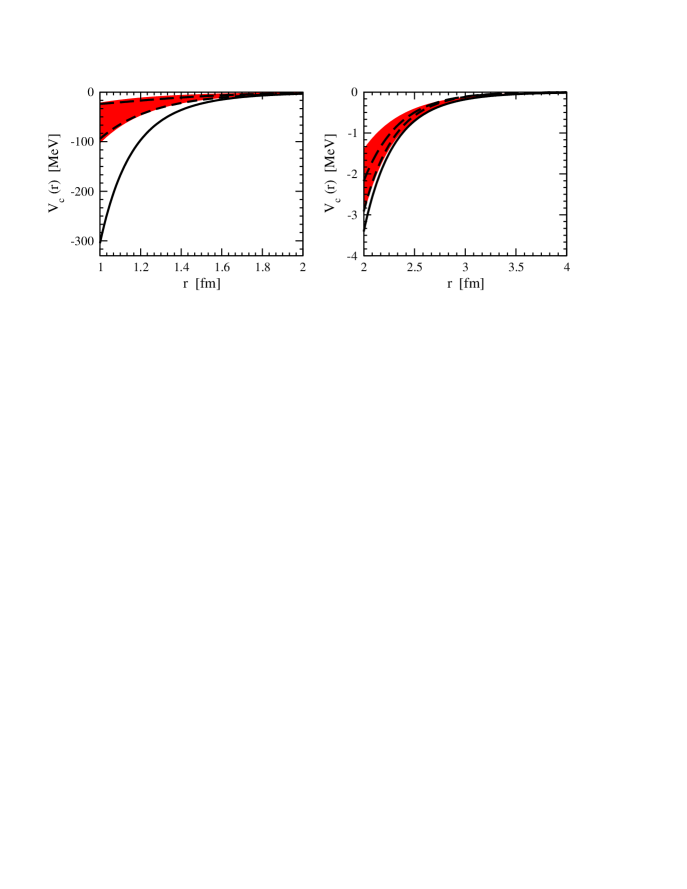
Figure 6: The potential $V_{C}$ in $r$–space. The solid line (band) shows the DR (SFR, $\tilde{\Lambda}=500\ldots 800$ MeV) result. The short–dashed (long–dashed) line refers to the phenomenological $\sigma$ ($\sigma+\omega+\rho$) contributions based on the isospin triplet configuration space version (OBEPR) of the Bonn potential [155].

Clearly, the large–distance asymptotics of the potential, which is constrained in a nontrivial way by chiral symmetry of QCD, is unaffected by the cut–off procedure (provided $\tilde{\Lambda}\gg M_{\pi}$). The strongest effects of the cut–off are observed at intermediate and shorter distances, where 2PE becomes unphysically attractive if DR is used. In contrast, removing the large components in the mass spectrum of the 2PE with the reasonably chosen cut–off $\tilde{\Lambda}=500\ldots 800$ MeV greatly reduces this attraction and yields the potential of the same order in magnitude as the one obtained in phenomenological boson–exchange models. We will see in section 4.1.1 how a choice of regularization affects the results for peripheral NN scattering at N²LO.

We further stress that other regularization schemes may be applied as well. For example, one can regularize divergent loop integrals using an ordinary momentum–space cut–off. The prominent feature of the SFR scheme is given by the fact that it only affects the two–nucleon contact interactions. One can, therefore, directly adopt the values for various LECs resulting from the single–nucleon sector analyses, where dimensional regularization has been used. This, in general, is not the case for a finite momentum cut–off regularization.

3.2.2 Pion–exchange contributions

Consider now pion–exchange contributions to the potential

$$V_{\pi}=V_{1\pi}+V_{2\pi}+V_{3\pi}+\ldots\,,$$ (3.30)

where one–, two– and three–pion exchange (3PE) contributions $V_{1\pi}$, $V_{2\pi}$ and $V_{3\pi}$ can be written in the low–momentum expansion as

$$V_{1\pi} = V_{1\pi}^{(0)}+V_{1\pi}^{(2)}+V_{1\pi}^{(3)}+V_{1\pi}^{(4)}+\ldots\,,$$

$$V_{2\pi} = V_{2\pi}^{(2)}+V_{2\pi}^{(3)}+V_{2\pi}^{(4)}+\ldots\,,$$

$$V_{3\pi} = V_{3\pi}^{(4)}+\ldots\,.$$ (3.31)

Here, the superscripts denote the corresponding chiral order and the ellipses refer to $(Q/\Lambda)^{5}$– and higher order terms. Contributions due to the exchange of four– and more pions are further suppressed: $n$–pion exchange diagrams start to contribute at the order $(Q/\Lambda)^{2n-2}$. Notice further that in this section we restrict ourselves to isopin–invariant contributions. Isospin–breaking corrections will be discussed in section 3.2.5. The corresponding relativistic corrections will be considered in section 3.2.4.

The static 1PE potential at N³LO has the form

$$V_{1\pi}^{(0)}+V_{1\pi}^{(2)}+V_{1\pi}^{(3)}+V_{1\pi}^{(4)}=-\biggl{(}\frac{g_{A}}{2F_{\pi}}\biggr{)}^{2}\,(1+\delta)^{2}\,\mbox{\boldmath$\tau$}_{1}\cdot\mbox{\boldmath$\tau$}_{2}\,\frac{\vec{\sigma}_{1}\cdot\vec{q}\,\vec{\sigma}_{2}\cdot\vec{q}}{\vec{q}\,^{2}+M_{\pi}^{2}}\,.$$ (3.32)

Here $\delta$ denotes an isospin–conserving Goldberger–Treiman discrepancy

$$\delta=-\frac{2d_{18}}{g_{A}}M_{\pi}^{2}+\kappa M_{\pi}^{4}\,,$$ (3.33)

where $d_{18}$ is a LEC from the dimension three $\pi N$ Lagrangian and the constant $\kappa$ determines the size of the first correction to the Goldberger–Treiman discrepancy. Here and in what follows, the expressions for the nuclear force should be understood as operators with respect to spin and isospin quantum numbers and matrix elements with respect to momentum variables. We further stress that all one– and two–loop $1\pi$–exchange diagrams at this order lead to renormalization of various LECs without introducing any form–factor–like behavior. The derivation of the 1PE potential to one loop in the method of unitary transformation is discussed in detail in Ref. [134].

We now turn to the 2PE contributions. It is convenient to express $V_{2\pi}$ in the CMS in the form:

$$V_{2\pi} = V_{C}+\mbox{\boldmath$\tau$}_{1}\cdot\mbox{\boldmath$\tau$}_{2}\,W_{C}+\left[V_{S}+\mbox{\boldmath$\tau$}_{1}\cdot\mbox{\boldmath$\tau$}_{2}\,W_{S}\right]\,\vec{\sigma}_{1}\cdot\vec{\sigma}_{2}+\left[V_{T}+\mbox{\boldmath$\tau$}_{1}\cdot\mbox{\boldmath$\tau$}_{2}\,W_{T}\right]\,\vec{\sigma}_{1}\cdot\vec{q}\,\vec{\sigma}_{2}\cdot\vec{q}$$

$$+ \left[V_{LS}+\mbox{\boldmath$\tau$}_{1}\cdot\mbox{\boldmath$\tau$}_{2}\,W_{LS}\right]\,i(\vec{\sigma}_{1}+\vec{\sigma}_{2})\cdot(\vec{q}\times\vec{k})+\left[V_{\sigma L}+\mbox{\boldmath$\tau$}_{1}\cdot\mbox{\boldmath$\tau$}_{2}\,W_{\sigma L}\right]\,\vec{\sigma}_{1}\cdot(\vec{q}\times\vec{k})\vec{\sigma}_{2}\cdot(\vec{q}\times\vec{k})\,,$$

where the superscripts $C$, $S$, $T$, $LS$ and $\sigma L$ of the scalar functions $V_{C}$, $\ldots$, $W_{\sigma L}$ refer to central, spin–spin, tensor, spin–orbit and quadratic spin–orbit components, respectively. The chiral 2PE potential $V_{2\pi}^{(2)}+V_{2\pi}^{(3)}$ is discussed in [140, 142, 131, 139] and in [119] using an energy–dependent formalism. For a related work see also [156]. The NLO 2PE potential is given by the contributions of the box, crossed–box, triangle and football diagrams shown in the first line of Fig. 7 which in the energy–independent formulation read

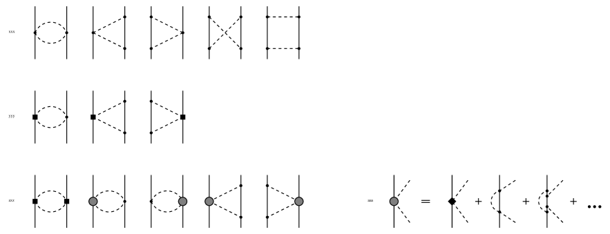
Figure 7: Leading, subleading and sub-subleading contributions to the chiral $2\pi$–exchange potential. Solid (dashed) lines correspond to nucleons (pions). Solid dots, filled rectangles and filled diamonds represent vertices with $\Delta_{i}=0$, $1$ and $2$, respectively. Shaded blob denotes the next–to–next–to–leading order contribution to the pion–nucleon scattering amplitude.

$$W_{C}^{(2)}(q) = -\frac{1}{384\pi^{2}F_{\pi}^{4}}\,L^{\tilde{\Lambda}}(q)\,\biggl{\{}4M_{\pi}^{2}(5g_{A}^{4}-4g_{A}^{2}-1)+q^{2}(23g_{A}^{4}-10g_{A}^{2}-1)+\frac{48g_{A}^{4}M_{\pi}^{4}}{4M_{\pi}^{2}+q^{2}}\biggr{\}}\,,$$

$$V_{T}^{(2)}(q) = -\frac{1}{q^{2}}V_{S}^{(2)}(q)=-\frac{3g_{A}^{4}}{64\pi^{2}F_{\pi}^{4}}\,L^{\tilde{\Lambda}}(q)\,.$$ (3.35)

Here, the loop function $L^{\tilde{\Lambda}}(q)$ is given by

$$L^{\tilde{\Lambda}}(q)=\theta(\tilde{\Lambda}-2M_{\pi})\,\frac{\omega}{2q}\,\ln\frac{\tilde{\Lambda}^{2}\omega^{2}+q^{2}s^{2}+2\tilde{\Lambda}q\omega s}{4M_{\pi}^{2}(\tilde{\Lambda}^{2}+q^{2})}~{},\quad\quad\omega=\sqrt{q^{2}+4M_{\pi}^{2}}~{},\quad\quad s=\sqrt{\tilde{\Lambda}^{2}-4M_{\pi}^{2}}\,.$$ (3.36)

These expressions are based on the SFR approach. The corresponding DR expressions can be obtained taking the limit $\tilde{\Lambda}\to\infty$. We further emphasize that a significant part of the NLO 2PE contributions was considered much earlier in the context of meson theory of nuclear forces, see e.g. [157, 158, 159, 160]. At N²LO one has to take into account the contributions of the triangle and football graphs in the second line of Fig. 7 with a single insertion of the subleading $\pi\pi NN$ vertex. One finds:

$$V_{C}^{(3)}(q) = -\frac{3g_{A}^{2}}{16\pi F_{\pi}^{4}}\biggl{\{}2M_{\pi}^{2}(2c_{1}-c_{3})-c_{3}q^{2}\biggr{\}}(2M_{\pi}^{2}+q^{2})A^{\tilde{\Lambda}}(q)\,,$$

$$W_{T}^{(3)}(q) = -\frac{1}{q^{2}}W_{S}^{(3)}(q)=-\frac{g_{A}^{2}}{32\pi F_{\pi}^{4}}\,c_{4}(4M_{\pi}^{2}+q^{2})A^{\tilde{\Lambda}}(q)\,,$$ (3.37)

where the N²LO loop function $A^{\tilde{\Lambda}}(q)$ has been defined in Eq. (3.24).

The N³LO corrections to the 2PE potential $V_{2\pi}^{(4)}$ have been recently calculated by Kaiser [145] and are schematically depicted in the third line of Fig. 7. They arise from two groups of diagrams, the one–loop football graphs with both dimension two $\pi\pi NN$ vertices of the $c_{1,\ldots,4}$–type and the diagrams which contain the third order pion–nucleon amplitude and lead to one–loop and two–loop graphs. We begin with the first group of corrections, for which one finds:

$$V_{C}^{(4)}(q) = \frac{3}{16\pi^{2}F_{\pi}^{4}}\,L^{\tilde{\Lambda}}(q)\,\left\{\left[\frac{c_{2}}{6}\omega^{2}+c_{3}(2M_{\pi}^{2}+q^{2})-4c_{1}M_{\pi}^{2}\right]^{2}+\frac{c_{2}^{2}}{45}\omega^{4}\right\}\,,$$

$$W_{T}^{(4)}(q) = -\frac{1}{q^{2}}W_{S}^{(4)}(q)=\frac{c_{4}^{2}}{96\pi^{2}F_{\pi}^{4}}\omega^{2}\,L^{\tilde{\Lambda}}(q)\,.$$ (3.38)

The expressions for the second group of corrections were obtained by Kaiser [145] and are given in appendix A in terms of the corresponding spectral functions.

Figure 8: Leading contributions to the $3\pi$–exchange potential. For notation see Fig. 7.

Three–pion exchange starts to contribute at N³LO and is given by diagrams shown in Fig. 8. The corresponding expressions for the spectral functions and the potential (obtained using dimensional regularization) have been given by Kaiser in [143, 144], see also [161] for a related work. It has been pointed out in these references that the resulting 3PE potential is much weaker than the N³LO 2PE contributions at physically interesting distances $r>1$ fm. Having the explicit expressions for the 3PE spectral functions, it is easy to calculate the potential in the SFR scheme. It is obvious, even without performing the explicit calculations, that the finite–range part of the 3PE potential in the SFR scheme is strongly suppressed at intermediate and short distances compared to the result obtained using DR. This is because the short range components which dominate the 3PE spectrum are explicitly excluded in this approach. This is exemplified in Fig. 9 for the case of the N³LO isoscalar spin–spin contribution proportional to $g_{A}^{4}$, which has been found in [143, 144] to yield the strongest 3PE potential for $0.6$ fm $<r<$ $1.4$ fm. For $r>0.5$ fm, it reaches at most $2\%-8\%$ (depending on the choice of the spectral function cut–off) of the corresponding N³LO 2PE contribution [162]. Similar results have been found for other leading 3PE contributions [143, 144]. For that reason the 3PE contributions have been neglected in the present N³LO analyses [163, 162]. Notice, however, that the potential resulting from subleading (i.e. N⁴LO) 3PE diagrams proportional to LECs $c_{i}$ and obtained using DR was found to be sizable at intermediate distances [164]. The strength of the 2PE and 3PE contributions considered above and the corresponding expressions in coordinate space are discussed in detail in Refs. [142, 144, 143, 165, 145].

3.2.3 Contact terms

The short–range part of the potential is represented by a series of contact interactions

$$V_{\rm cont}=V^{(0)}_{\rm cont}+V^{(2)}_{\rm cont}+V^{(4)}_{\rm cont}+\ldots~{},$$ (3.39)

where the superscripts denote the corresponding chiral order as defined in Eq. (2.47). These terms feed into the matrix–elements of the two S–, P– and D–waves and the two lowest transition potentials in the following way:

$$\langle S|V_{\rm cont}|S\rangle = \tilde{C}_{S}+C_{S}(p^{2}+p^{\prime 2})+D_{S}^{1}\,p^{2}\,{p^{\prime}}^{2}+D_{S}^{2}\,({p}^{4}+{p}^{\prime 4})~{},$$

$$\langle P|V_{\rm cont}|P\rangle = C_{P}\,p\,p^{\prime}+D_{P}\,p\,p^{\prime}\,({p}^{2}+p^{\prime}\,{}^{2})~{},$$

$$\langle D|V_{\rm cont}|D\rangle = D_{D}\,{p}^{2}\,{p}^{\prime 2}~{},$$

$$\langle^{3}S_{1}|V_{\rm cont}|^{3}D_{1}\rangle = C_{3D1-3S1}\,p^{2}+D_{3D1-3S1}^{1}\,{p}^{2}\,{p}^{\prime 2}+D_{3D1-3S1}^{2}\,p^{4}~{},$$

$$\langle^{3}D_{1}|V_{\rm cont}|^{3}S_{1}\rangle = C_{3D1-3S1}\,{p^{\prime}}^{2}+D_{3D1-3S1}^{1}\,{p}^{2}\,{p}^{\prime 2}+D_{3D1-3S1}^{2}\,{p^{\prime}}^{4}~{},$$

$$\langle^{3}P_{2}|V_{\rm cont}|^{3}F_{2}\rangle = D_{3F2-3P2}\,{p}^{3}\,{p}^{\prime}~{},$$

$$\langle^{3}F_{2}|V_{\rm cont}|^{3}P_{2}\rangle = D_{3F2-3P2}\,{p}\,{p^{\prime}}^{3}~{},$$ (3.40)

where $p=|\vec{p}\,|$, ${p}^{\prime}=|\vec{p}\,^{\prime}|$ and the subscripts $S=\{1S0,\,3S1\}$, $P=\{1P1,\,3P0,\,3P1,\,3P2\}$, $D=\{1D2,\,3D1,\,3D2,\,3D3\}$ refer to the corresponding channel. The relations between the spectroscopic LECs in the above equations and the ones that occur in the Lagrangian can be found in [162]. Isospin–breaking short–range corrections will be specified in section 3.2.5.

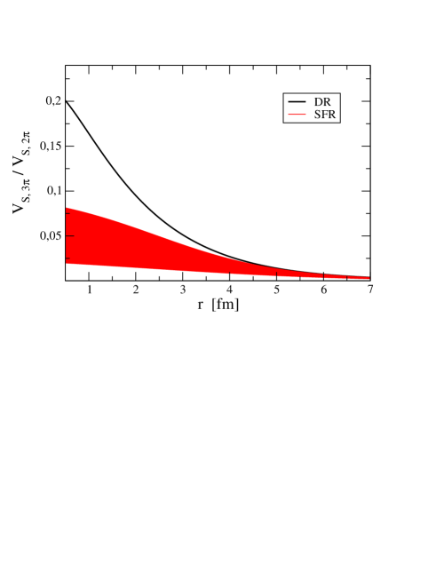
Figure 9: The ratio of the isoscalar spin–spin 3PE and 2PE N³LO contributions using dimensional and spectral function regularization. The cut–off in the spectral function varies in the range $\tilde{\Lambda}=500\ldots 700$ MeV.

3.2.4 Relativistic corrections

The first relativistic corrections to the nuclear force appear at order $\nu=4$ provided that the nucleon mass is counted according to Eq. (2.49). They result from both $1/m^{2}$–corrections to the static 1PE potential and $1/m$–corrections to the order $\nu=2$ static 2PE potential. In addition, at this order one also needs to correct the nonrelativistic expression for the nucleon kinetic energy

$$E_{\rm kin}=\sqrt{\vec{p}\,^{2}+m^{2}}-m\sim\frac{\vec{p}\,^{2}}{2m}-\frac{\vec{p}\,^{4}}{8m^{3}}\,,$$ (3.41)

which enters the corresponding dynamical equation. Equivalently, one can use the full, not expanded expression for the nucleon kinetic energy which leads to the following Schrödinger equation for two nucleons in the CMS:

$$\left[\left(2\sqrt{\vec{p}\,^{2}+m^{2}}-2m\right)+V\right]\Psi=E\Psi\,,$$ (3.42)

where $m=m_{p}$ for the $pp$, $m=m_{n}$ for the $nn$ and $m=2m_{p}m_{n}/(m_{p}+m_{n})$ for the $np$ case, see [162] for more details on the kinematics. Notice that Eq. (3.42) can be cast into equivalent nonrelativistic forms, i.e. into the Schrödinger equations with the nucleon kinetic energy $E_{\rm kin}=\vec{p}\,^{2}/(2m)$ [146, 166]. The advantage of Eq. (3.42) versus the corresponding nonrelativistic forms is that it can easily be generalized to the case of three and more nucleons. Changing the form of the Schrödinger equation causes changes in the relativistic corrections to the nuclear potential. Relativistic corrections to the interaction can, therefore, only be defined within a particular framework. For the Schrödinger equation (3.42), the corrections to the leading 1PE potential $V_{1\pi}^{(0)}$ take in the NN CMS the form:

$$V_{1\pi}^{(4)}=-\left(\frac{\vec{p}\,^{2}+\vec{p}\,^{\prime}{}^{2}}{2m^{2}}\right)V_{1\pi}^{(0)}\,,$$ (3.43)

where $\vec{p}$ and $\vec{p}\,^{\prime}$ are the NN initial and final CMS momenta. This choice of corrections is sometimes called the “minimal nonlocality” choice, see [146] and references therein. The corresponding $1/m$–corrections to the 2PE potential read:

$$V_{C}^{(4)}(q) = \frac{3g_{A}^{4}}{512\pi mF_{\pi}^{4}}\bigg{\{}\frac{2M_{\pi}^{5}}{\omega^{2}}-3(4M_{\pi}^{4}-q^{4})A^{\tilde{\Lambda}}(q)\bigg{\}}\,,$$

$$W_{C}^{(4)}(q) = \frac{g_{A}^{2}}{128\pi mF_{\pi}^{4}}\Bigg{\{}\frac{3g_{A}^{2}M_{\pi}^{5}}{\omega^{2}}-\bigg{[}4M_{\pi}^{2}+2q^{2}-g_{A}^{2}\left(7M_{\pi}^{2}+\frac{9}{2}q^{2}\right)\bigg{]}(2M_{\pi}^{2}+q^{2})A^{\tilde{\Lambda}}(q)\Bigg{\}}\,,$$

$$V_{T}^{(4)}(q) = -\frac{1}{q^{2}}V_{S}^{(4)}(q)=\frac{9g_{A}^{2}}{512\pi mF_{\pi}^{4}}\left(4M_{\pi}^{2}+\frac{3}{2}q^{2}\right)A^{\tilde{\Lambda}}(q)\,,$$

$$W_{T}^{(4)}(q) = -\frac{1}{q^{2}}W_{S}^{(4)}(q)=-\frac{g_{A}^{2}}{256\pi mF_{\pi}^{4}}\left[8M_{\pi}^{2}+2q^{2}-g_{A}^{2}\left(8M_{\pi}^{2}+\frac{5}{2}q^{2}\right)\right]A^{\tilde{\Lambda}}(q)\,,$$

$$V_{LS}^{(4)}(q) = -\frac{3g_{A}^{4}}{64\pi mF_{\pi}^{4}}(2M_{\pi}^{2}+q^{2})A^{\tilde{\Lambda}}(q)\,,$$

$$W_{LS}^{(4)}(q) = -\frac{g_{A}^{2}(1-g_{A}^{2})}{64\pi mF_{\pi}^{4}}(4M_{\pi}^{2}+q^{2})A^{\tilde{\Lambda}}(q)\,.$$ (3.44)

Notice that the above expressions differ from the ones given in [142] due to the different form of the dynamical equation and relativistic corrections to the 1PE potential employed in the present work. For an extensive discussion of this issue the reader is referred to Ref. [146] where the dependence of relativistic corrections on certain kinds of unitary transformations is studied and the general expressions for $1/m^{2}$–corrections to the 1PE potential and $1/m$–corrections to the leading 2PE potential are obtained. We further stress that if the nucleon mass is counted, contrary to Eq. (2.49), as $m\sim\Lambda$, $1/m^{4}$–corrections to the 1PE potential, $1/m^{2}$–corrections to the order $\nu=2$ 2PE potential and $1/m$–corrections to the order $\nu=3$ 2PE potential have to be taken into account at N³LO in addition to terms shown in Eqs. (3.43), (3.2.4). The corresponding expressions can be found in [165].

3.2.5 Isospin–breaking corrections

Within the Standard Model, isospin violation has its origin in the different masses of the up and down quarks and the electromagnetic interactions. Consider first isospin–breaking in the strong interactions. The QCD quark mass term can be expressed in the two–flavor case as:

$${\cal L}_{\rm mass}^{\rm QCD}=-\frac{1}{2}\bar{q}\,(m_{\rm u}+m_{\rm d})(1+\epsilon\tau_{3})\,q~{},\quad\quad\quad\mbox{where}\quad\quad\epsilon\equiv{m_{u}-m_{d}\over m_{u}+m_{d}}\sim-{1\over 3}\,.$$ (3.45)

The above numerical estimation corresponds to the light quark mass values based on a modified $\overline{\rm MS}$ subtraction scheme at a renormalization scale of 1 GeV [8]. The isovector term ($\propto\tau_{3}$) in Eq. (3.45) breaks isospin symmetry and generates a series of isospin–breaking effective interactions $\propto(\epsilon M^{2}_{\pi})^{n}$ with $n\geq 1$. It is, therefore, natural to count strong isospin violation in terms of $\epsilon M^{2}_{\pi}$ [121]. Electromagnetic terms in the effective Lagrangian can be generated using the method of external sources, see e.g. [167, 168, 169, 170] for more details. All such terms are proportional to the nucleon charge matrix $Q_{\rm ch}=e\,(1+\tau_{3})/2$, where $e$ denotes the electric charge. More precisely, the vertices which contain (do not contain) the photon fields are proportional to $Q^{n}_{\rm ch}$ ($Q^{2n}_{\rm ch}$), where $n=1,2,\ldots$. For processes in the absence of external fields, in which no photon can leave a Feynman diagram, it is convenient to introduce the small parameter $e^{2}\sim 1/10$ for isospin–violating effects caused by the electromagnetic interactions. Isospin–violating terms in the effective Lagrangian at lowest orders can be found in [121, 122, 123, 124], see also Ref. [125].

Isospin–breaking nuclear forces can, in principle, be derived in the EFT framework performing independent expansions in $Q/\Lambda$, $\epsilon$ and $e$. It is, however, convenient to relate these small parameters with each other in order to have a single expansion parameter. In Ref. [125], the following counting rules were adopted:

$$\epsilon\sim e\sim\frac{Q}{\Lambda},\quad\quad\frac{e^{2}}{(4\pi)^{2}}\sim\frac{Q^{4}}{\Lambda^{4}}\,.$$ (3.46)

The power counting expression in Eq. (2.47) can be easily extended to include the contributions due to $n_{\gamma}$ virtual photons:

$$\nu=-2+2n_{\gamma}+2N+2(L-C)+\sum_{i}V_{i}\Delta_{i}\,.$$ (3.47)

Here, the $Q$–power $\Delta_{i}$ of the vertex $i$ defined in Eq. (2.47) has to be adjusted according to the rules given in Eq. (3.46). It should be understood that the counting rules on Eq. (3.46) are by no means unique and represent an attempt to relate the sizes of the isospin–breaking and isospin–conserving nuclear forces with each other in a realistic way. Different rules are usually adopted in the meson and single–nucleon sectors, see e.g. [122, 123, 124]. Counting rules very similar to the ones in Eq. (3.46) (but not exactly the same) have been used in applications in the 2N sector in Refs. [121, 171, 172, 173, 174, 175]. Clearly, changing the counting rules shifts various nuclear force contributions to different orders but does not affect their explicit form. The most realistic set of counting rules, i.e. the one that finally leads to the most natural values of the LECs, can only be figured out in practical calculations.

The 2N forces fall in to four classes with respect to their isospin structure [176]:

$$\begin{array}[]{lcl}\mbox{Class I:}&\mbox{\hskip 28.45274pt}&V_{\rm I}=\alpha_{\rm I}+\beta_{\rm I}\,\mbox{\boldmath$\tau$}_{1}\cdot\mbox{\boldmath$\tau$}_{2}\,,\\[2.58334pt] \mbox{Class II:}&&V_{\rm II}=\alpha_{\rm II}\,\tau_{1}^{3}\,\tau_{2}^{3}\,,\\[2.58334pt] \mbox{Class III:}&&V_{\rm III}=\alpha_{\rm III}\,(\tau_{1}^{3}+\tau_{2}^{3})\,,\\[2.58334pt] \mbox{Class IV:}&&V_{\rm IV}=\alpha_{\rm IV}\,(\tau_{1}^{3}-\tau_{2}^{3})+\beta_{\rm IV}\,[\mbox{\boldmath$\tau$}_{1}\times\mbox{\boldmath$\tau$}_{2}]^{3}\,,\end{array}$$ (3.48)

where $\alpha_{\rm i}$, $\beta_{\rm i}$ are space and spin operators. The operator $\beta_{\rm IV}$ has to be odd under a time reversal transformation. While class (I) forces are isospin–invariant, all other classes (II), (III) and (IV) forces are isospin–breaking. Class (II) forces, $V_{\rm II}$, maintain charge symmetry but break charge independence. They are usually referred to as charge independence breaking (CIB) forces. Class (III) forces break charge symmetry but do not lead to isospin mixing in the 2N system. Finally, class (IV) forces break charge symmetry and cause isospin mixing in the 2N system.

We will now discuss various contributions to the isospin–violating 2N force which have been extensively studied in the chiral EFT framework and worked out up to order $\nu=5$. It can be expressed as:

$$V_{\rm 2N}^{I}=V_{\rm EM}+V_{\pi\gamma}+V_{1\pi}^{I}+V_{2\pi}^{I}+V_{\rm cont}^{I}\,,$$ (3.49)

where the terms in the right–hand side refer to the long–range electromagnetic force, pion–photon exchange, isospin–breaking one– and two–pion exchange potentials and contact terms, respectively. The superscript $I$ is used in order to distinguish the isospin–breaking from the corresponding isospin–invariant contributions considered in sections 3.2.2, 3.2.3. Let us first comment on the long–range electromagnetic force whose dominant contribution is given by the static Coulomb interaction at order $\nu=2$. The first long–range corrections are suppressed by $m^{-2}$ (relativistic corrections to the static one–photon exchange). At this order, the long–range electromagnetic NN interaction is given by

$$V_{\rm EM}(pp) = V_{\rm C1}+V_{\rm C2}+V_{\rm VP}+V_{\rm MM}(pp)\,,$$

$$V_{\rm EM}(np) = V_{\rm MM}(np)\,,$$

$$V_{\rm EM}(nn) = V_{\rm MM}(nn)\,,$$ (3.50)

where $V_{\rm C1}$ and $V_{\rm C2}$ are usually referred to as “improved Coulomb potential”. They include the relativistic $1/m^{2}$–corrections to the static Coulomb potential worked out in Ref. [177]. The expressions for the vacuum polarization potential $V_{\rm VP}$ and magnetic moment interaction $V_{\rm MM}$ can be found in Refs. [178, 179] and [180], respectively. Notice that $V_{\rm EM}$ contains classes (II), (III) and (IV) forces. The class (IV) force is given exclusively by the magnetic moment interaction. We also stress that the effects of $V_{\rm EM}$ are enhanced at low energy due to the long–range nature of this force. Even the effects due to $V_{\rm MM}$, which is suppressed by factor $\sim(Q/m)^{2}$ compared to the static Coulomb interaction and thus contributes at order $\nu=6$, might be large for certain scattering observables under specific kinematical conditions, see e.g. [180].

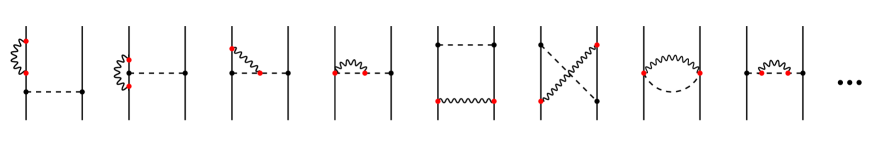
Figure 10: One–loop $\pi\gamma$ diagrams contributing to the isospin–breaking NN force of the 1PE range. Wavy lines represent photons. Solid dots refer to the leading strong and electromagnetic vertices. Only one representative topology is depicted for each graph. For the remaining notation see Fig. 7.

The one–loop diagrams contributing to the isospin–breaking NN force of the 1PE range are shown in Fig. 10 and were considered by van Kolck et al. [181]. Some of the graphs depicted in this figure lead to renormalization of the isospin–breaking 1PE potential (i.e. change its strength). Notice further that due to isospin, only charged pion exchange can contribute to the $\pi\gamma$ potential $V_{\pi\gamma}$ and thus it only affects the $np$ system. The resulting $\pi\gamma$ potential is CIB and has the form

$$V_{\pi\gamma}(\vec{q}\,) = -{g_{A}^{2}\over 4F_{\pi}^{2}M_{\pi^{+}}^{2}}\,(\mbox{\boldmath$\tau$}_{1}\cdot\mbox{\boldmath$\tau$}_{2}-\tau_{1}^{3}\,\tau_{2}^{3})\,\vec{\sigma}_{1}\cdot\vec{q}\,\vec{\sigma}_{2}\cdot\vec{q}\,\,V_{\pi\gamma}(\beta)~{},$$

$$V_{\pi\gamma}(\beta) = {\alpha\over\pi}\biggl{[}-{(1-\beta^{2})^{2}\over 2\beta^{4}(1+\beta^{2})}\ln(1+\beta^{2})+{1\over 2\beta^{2}}-{2\bar{\gamma}\over 1+\beta^{2}}\biggr{]}~{}.$$ (3.51)

Here, $\beta=|\vec{q}\,|/M_{\pi^{+}}$ and $\bar{\gamma}$ is a regularization scheme dependent constant. The analytical form of $V_{\pi\gamma}$ is similar to the one of the 1PE potential but differs in strength by the factor $\alpha/\pi\simeq 1/400$.

Isospin–breaking corrections to the 1PE potential were extensively studied within the EFT framework [121, 172, 175, 125]. It is convenient to express the static 1PE potential in Eq. (3.32) in a more general form, which already incorporates some (but not all) of the isospin–breaking corrections:

$$V_{1\pi}+V_{1\pi}^{I}(pp)\, = (1+\delta_{p})^{2}\,V(M_{\pi^{0}})\,,$$

$$V_{1\pi}+V_{1\pi}^{I}(nn) = (1+\delta_{n})^{2}\,V(M_{\pi^{0}})\,,$$

$$V_{1\pi}+V_{1\pi}^{I}(np)\, = -(1+\delta_{p})(1+\delta_{n})\,V(M_{\pi^{0}})+(-1)^{T+1}\,2(1+\delta_{c})^{2}\,V(M_{\pi^{\pm}})\,,$$ (3.52)

where we utilize the notation of Ref. [125]. In Eq. (3.2.5), $T=0,1$ denotes the total isospin of the two–nucleon system and $V(M_{{}_{i}})$ is defined as:

$$V(M_{i})=-\biggl{(}\frac{g_{A}}{2F_{\pi}}\biggr{)}^{2}\,\frac{(\vec{\sigma}_{1}\cdot\vec{q}\,)(\vec{\sigma}_{2}\cdot\vec{q}\,)}{\vec{q}\,^{2}+M_{i}^{2}}\,.$$ (3.53)

The constants $\delta_{p}$, $\delta_{n}$ and $\delta_{c}$ in Eq. (3.2.5) specify the isospin dependence of the pion–nucleon coupling constant. For the isospin–symmetric 1PE potential, the quantity $\delta_{p}=\delta_{n}=\delta_{c}$ gives an isospin–conserving Goldberger–Treiman discrepancy. Charge–symmetry conservation implies $\delta_{p}=\delta_{n}\neq\delta_{c}$. The leading isospin–breaking contribution to the pion–nucleon coupling constants is of the strong origin and leads to the class (III) force at order $\nu=3$. Up to order $\nu=5$, isospin–violating contributions to $\delta_{i}$’s result from various tree– and one–loop diagrams and lead to both classes (II) and (III) forces, see [172, 125] for more details. Apart from the corrections due to $\delta_{p}\neq\delta_{n}\neq\delta_{c}$, the expressions for the 1PE potential in Eq. (3.2.5) also incorporate the order $\nu=2$ class (II) contribution due to the mass difference of the exchanged pions, $\delta M_{\pi}^{2}=M_{\pi^{\pm}}^{2}-M_{\pi^{0}}^{2}=(36\mbox{ MeV})^{2}$. This is, in fact, the dominant contribution to the isospin–breaking nuclear force. Clearly, the corrections $\propto(\delta M_{\pi}^{2})^{2}$ at order $\nu=4$ are also included in Eq. (3.2.5). Further contributions to the isospin–breaking 1PE potential not included in Eq. (3.2.5) arise at order $\nu=4$ due to the proton–to–neutron mass difference, $\delta m=m_{p}-m_{n}=-1.29$ MeV, and are given by [175, 125]

$$V_{1\pi}^{I}{}^{(4)} = -i\frac{\delta m}{2m}\left(\frac{g_{A}}{2F_{\pi}}\right)^{2}[\mbox{\boldmath$\tau$}_{1}\times\mbox{\boldmath$\tau$}_{2}]^{3}\,\frac{1}{(\vec{q_{1}}^{2}+M_{\pi}^{2})}\Bigg{[}\frac{(\vec{\sigma}_{1}\cdot\vec{q}_{1}\,)(\vec{\sigma}_{2}\cdot\vec{q}_{1}\,)}{(\vec{q_{1}}^{2}+M_{\pi}^{2})}(\vec{p_{1}}^{2}-\vec{p_{2}}^{2}-{\vec{p_{1}}^{\prime}}{}^{2}+{\vec{p_{2}}^{\prime}}{}^{2})$$ (3.54)

$${}-\Big{(}(\vec{\sigma}_{1}\cdot\vec{q}_{1})(\vec{\sigma}_{2}\cdot(\vec{p}_{2}+\vec{p_{2}}^{\prime}))+(\vec{\sigma}_{1}\cdot(\vec{p}_{1}+\vec{p_{1}}^{\prime}))(\vec{\sigma}_{2}\cdot\vec{q}_{1})\Big{)}\Bigg{]}\,,$$

where $\vec{p}_{i}$ ($\vec{p}_{i}\,^{\prime}$) denotes the incoming (outgoing) momentum of the nucleon $i$ and $\vec{q}_{1}=\vec{p_{1}}^{\prime}-\vec{p}_{1}=-(\vec{p_{2}}^{\prime}-\vec{p_{2}})$. Notice that the first term in the square bracket vanishes in the CMS. The potential in Eq. (3.54) represents the dominant class (IV) force. The dependence of $V_{1\pi}^{I}{}^{(4)}$ on the total momentum of the 2N system is explained in [175]. In addition to the corrections linear in $\delta m/m$ in Eq. (3.54), one has to take into account the CIB contribution $\propto(\delta m)^{2}$ which reads [180, 121, 175, 125]:

$$V_{\rm 1\pi}^{I}{}^{(4)}=-(\delta m)^{2}\left(\frac{g_{A}}{2F_{\pi}}\right)^{2}\left(\mbox{\boldmath$\tau$}_{1}\cdot\mbox{\boldmath$\tau$}_{2}-\tau_{1}^{3}\tau_{2}^{3}\right)\,\frac{(\vec{\sigma}_{1}\cdot\vec{q}\,)(\vec{\sigma}_{2}\cdot\vec{q}\,)}{(\vec{q}\,^{2}+M_{\pi}^{2})^{2}}\,.$$ (3.55)

Notice that the isospin–violating piece has the same structure as the correction due to the pion mass difference at order $\nu=2$ but is $\delta M_{\pi}^{2}/(\delta m)^{2}\sim 660$ times weaker. No new structures in the 1PE potential appear at order $\nu=5$.

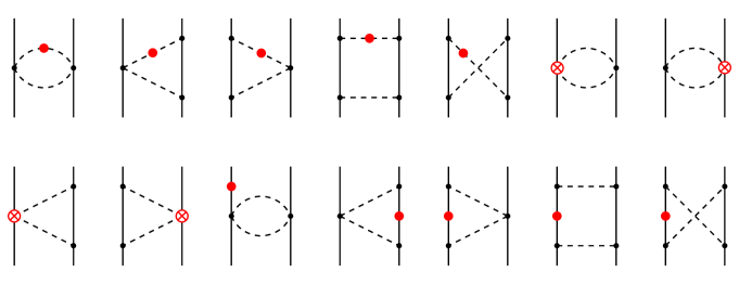
Figure 11: Leading isospin–breaking corrections to the 2PE potential. A light–shaded circle inserted at a pion (nucleon) line refers to a single insertion of the pion (nucleon) mass difference. Crossed circles denote the leading isospin–breaking $\pi\pi NN$ vertices of dimension $\Delta_{i}=2$. For graphs with pion/nucleon mass difference insertions, only one representative topology is depicted. For remaining notation see Fig. 7.

Let us now switch to the 2PE potential. The dominant contributions arise at order $\nu=4$ from 1–loop diagrams constructed from the leading $\pi NN$ and $\pi\pi NN$ vertices and a single insertion of the pion mass difference, the proton–to–neutron mass shift or the order $\Delta_{i}=2$ isospin–breaking $\pi\pi NN$ vertex. The corresponding diagrams are shown in Fig. 11. Let us first discuss the class (II) contributions arising from diagrams with a single insertion of $\delta M_{\pi}^{2}$. As shown in Ref. [173], the potential can be expressed in terms of the corresponding isospin–invariant contributions given in Eq. (3.2.2) without performing any additional calculations. To that aim, one can first decompose the isospin–invariant 2PE potential in to the isoscalar and isovector pieces

$$V_{2\pi}=V_{2\pi}^{0}+V_{2\pi}^{1}\,\mbox{\boldmath$\tau$}_{1}\cdot\mbox{\boldmath$\tau$}_{2}~{}.$$ (3.56)

The leading isospin–breaking effects due to $M_{\pi^{\pm}}\neq M_{\pi^{0}}$ are incorporated properly if one uses $\tilde{M}_{\pi}$, defined as

$$\tilde{M}_{\pi}=\frac{2}{3}M_{\pi^{\pm}}+\frac{1}{3}M_{\pi^{0}}~{},$$ (3.57)

in the scalar part $V_{2\pi}^{0}$ and adopts for the isovector part:

$$\begin{array}[]{ll}V_{2\pi}^{1}(M_{\pi^{\pm}})&{\rm for}~{}~{}pp~{}~{}{\rm and}~{}~{}nn~{},\\[4.30554pt] V_{2\pi}^{1}(M_{\pi^{0}})&{\rm for}~{}~{}np,~{}~{}T=1~{},\\[4.30554pt] V_{2\pi}^{1}(\tilde{M}_{\pi})&{\rm for}~{}~{}np,~{}~{}T=0~{}.\end{array}$$ (3.58)

These results are valid modulo $(\delta M_{\pi}^{2}/M_{\pi}^{2})^{2}$–corrections which first contribute to the 2PE potential at order $\nu=6$. Clearly, one can also express the corresponding potential in a more traditional form in terms of isospin matrices and without referring to particular isospin channels, see Ref. [125].

All remaining 2PE contributions at order $\nu=4$ lead to class (III) forces and were derived independently and using different methods by several groups, see [182, 174, 125] and [183] for a related earlier work. One finds

$$V_{2\pi}^{I}{}^{(4)} = -\frac{g_{A}^{2}}{64\pi F_{\pi}^{4}}\,(\tau_{1}^{3}+\tau_{2}^{3})\,\left[\frac{2g_{A}^{2}\,\delta m\,M_{\pi}^{3}}{4M_{\pi}^{2}+q^{2}}-\Big{(}4g_{A}^{2}\,\delta m-(\delta m)^{\rm str}\Big{)}(2M_{\pi}^{2}+q^{2})\,A^{\Lambda}(q)\right]$$ (3.59)

$${}+\frac{g_{A}^{4}\,\delta m}{32\pi F_{\pi}^{4}}\,(\tau_{1}^{3}+\tau_{2}^{3})\,\left[(\vec{\sigma}_{1}\cdot\vec{q}\,)(\vec{\sigma}_{2}\cdot\vec{q}\,)-(\vec{\sigma}_{1}\cdot\vec{\sigma}_{2})\,\vec{q}^{\,2}\right]\,A^{\Lambda}(q)\,.$$

Here the LEC accompanying the order $\Delta_{i}=2$ isospin–breaking $\pi\pi NN$ vertex is expressed in terms of to the strong contribution $(\delta m)^{\rm str}$ to the nucleon mass shift $\delta m=(\delta m)^{\rm str}+(\delta m)^{\rm em}$, where

$$(\delta m)^{\rm str} = (m_{p}-m_{n})^{\rm str}=-2.05\pm 0.3\mbox{ MeV ,}$$

$$(\delta m)^{\rm em} = (m_{p}-m_{n})^{\rm em}=0.76\pm 0.3\mbox{ MeV .}$$ (3.60)

These values are taken from Ref. [184] and based on an evaluation of the Cottingham sum rule. Notice that the vertices corresponding to $(\delta m)^{\rm str}$ and $(\delta m)^{\rm em}$ have, according to the counting rules in Eq. (3.46), dimensions $\Delta_{i}=2$ and $3$, respectively. Notice further that some of the diagrams shown in Fig. 11, in particular the planar box and the football diagrams with a single insertion of $\delta m$, lead to vanishing contributions.

Consider now the subleading isospin–breaking 2PE potential which is due to 1–loop diagrams (some of which lead to vanishing results) shown in Fig. 12.

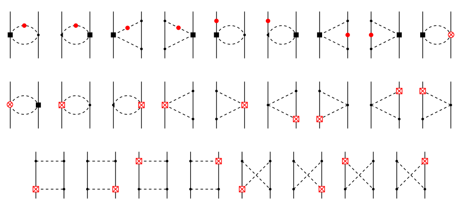
Figure 12: Subleading isospin–breaking corrections to the 2PE potential. Crossed rectangles denote isospin–breaking vertices of dimension $\Delta_{i}=3$. Graphs resulting from the interchange of the vertex ordering are not shown. For remaining notation see Figs. 7, 11.

The class (II) contributions $\propto\delta M_{\pi}^{2}$ can be obtained using Eq. (3.58) from the corresponding isospin–invariant 2PE potential in Eq. (3.2.2). The remaining terms were calculated recently using the method of unitary transformation [125]. The resulting class (III) potential reads:

$$V_{2\pi}^{I}{}^{(5)} = -\frac{1}{96\pi^{2}F_{\pi}^{4}}\,(\tau_{1}^{3}+\tau_{2}^{3})\,L^{\Lambda}(q)\,\bigg{\{}-g_{A}^{2}\,\delta m\frac{48M_{\pi}^{4}(2c_{1}+c_{3})}{4M_{\pi}^{2}+q^{2}}$$ (3.61)

$$\mbox{\hskip 56.9055pt}+4M_{\pi}^{2}\Big{[}g_{A}^{2}\,\delta m\,(18c_{1}+2c_{2}-3c_{3})+\Big{(}2\delta m-(\delta m)^{\rm str}\Big{)}\,(6c_{1}-c_{2}-3c_{3})\Big{]}$$

$$\mbox{\hskip 56.9055pt}+q^{2}\Big{[}g_{A}^{2}\,\delta m\,(5c_{2}-18c_{3})-\Big{(}2\delta m-(\delta m)^{\rm str}\Big{)}\,(c_{2}+6c_{3})\Big{]}\bigg{\}}$$

$${}-\frac{g_{A}^{2}}{16\pi^{2}F_{\pi}^{4}}\,(\tau_{1}^{3}+\tau_{2}^{3})\,\left[(\vec{\sigma}_{1}\cdot\vec{q}\,)(\vec{\sigma}_{2}\cdot\vec{q}\,)-(\vec{\sigma}_{1}\cdot\vec{\sigma}_{2})\,\vec{q}^{\,2}\right]\,L^{\Lambda}(q)\,\Big{(}\delta m\,c_{4}+g_{A}\,\beta\Big{)}\,,$$

where $\beta$ is a combination of the LECs accompanying the leading isospin–breaking $\pi NN$ vertex. At order $\nu=5$, it can be expressed in terms of the constants $\delta_{i}$ defined in Eq. (3.2.5) as $\beta=(1/4)(\delta_{p}-\delta_{n})g_{A}$. The complete expressions for the isospin–breaking 2PE potential in $r$–space can be found in [125].

Finally, isospin–breaking contact terms up to order $\nu=5$ feed in to the matrix–elements of the S– and P–waves in the following way:

$$\langle^{1}S_{0},\;pp\,|V_{\rm cont}^{I}|^{1}S_{0},\;pp\,\rangle = \tilde{\beta}_{1S0}^{pp}+\beta_{1S0}\,(p^{2}+p^{\prime 2})~{},$$

$$\langle^{1}S_{0},\,nn\,|V_{\rm cont}^{I}|^{1}S_{0},\,nn\,\rangle = \tilde{\beta}_{1S0}^{nn}-\beta_{1S0}\,(p^{2}+p^{\prime 2})~{},$$

$$\langle^{3}P_{0},\;pp\,|V_{\rm cont}^{I}|^{3}P_{0},\;pp\,\rangle = -\langle^{3}P_{0},\;nn\,|V_{\rm cont}^{I}|^{3}P_{0},\;nn\,\rangle=\beta_{3P0}\,\,p\,p^{\prime}~{},$$

$$\langle^{3}P_{1},\;pp\,|V_{\rm cont}^{I}|^{3}P_{1},\;pp\,\rangle = -\langle^{3}P_{1},\;nn\,|V_{\rm cont}^{I}|^{3}P_{1},\;nn\,\rangle=\beta_{3P1}\,\,p\,p^{\prime}~{},$$

$$\langle^{3}P_{2},\;pp\,|V_{\rm cont}^{I}|^{3}P_{2},\;pp\,\rangle = -\langle^{3}P_{2},\;nn\,|V_{\rm cont}^{I}|^{3}P_{2},\;nn\,\rangle=\beta_{3P2}\,\,p\,p^{\prime}~{},$$

$$\langle^{1}P_{1},\,np\,|V_{\rm cont}^{I}|^{3}P_{1},\,np\,\rangle = \beta_{1P1-3P1}\,\,p\,p^{\prime}~{},$$ (3.62)

where $\beta_{i}$, $\tilde{\beta}_{i}$ are the corresponding LECs. Here, we use the convention according to which the np matrix elements (with exception of the last term in Eq. (3.2.5)) do not change by switching off isospin–violating contact terms. Notice further that all terms quadratic in momenta are of the order $\nu=5$.

Last but not least, we would like to emphasize that chiral EFT supports the following hierarchy of the nuclear forces [121]: class (I) $>$ class (II) $>$ class (III) $>$ class (IV).

3.2.6 Towards a relativistic NN potential

In this section, we will discuss the problem with the formal inconsistency of the heavy–baryon (HB) expansion mentioned in section 2.1 and its impact on the nuclear potential and NN scattering. For that, consider the contribution to the NN scattering amplitude arising from the triangle diagrams in the second line of Fig. 7. We assume exact isospin symmetry throughout this section. Further, we follow closely the procedure of Ref. [185] and restrict ourselves to the central part of this contribution, which is proportional to the LECs $c_{1,3}$ and can be expressed in terms of the $\pi N$ scattering amplitude and the nuclear scalar form factor. For a discussion of the nuclear scalar form factor in relativistic CHPT, the reader is referred to Ref. [47], see also [58] for the results in the infrared regularized version of CHPT. Using the relativistic expression for the nucleon propagator and utilizing the notation of Ref. [185], this contribution to the scattering amplitude can be written as:

$$T_{C}^{rel}(t)=\frac{3mg_{A}^{2}}{16\pi^{2}F_{\pi}^{4}}\,\left(2M_{\pi}^{2}(2c_{1}-c_{3})+c_{3}t\right)\left[J_{c,c}(t)-J_{c,sN}^{(1)}(t)\right]\,.$$ (3.63)

Here, $t=q^{2}$, $q=p^{\prime}-p$ and the integrals $J_{c,c}(t)$ and $J_{c,sN}^{(1)}(t)$ read:

$$J_{c,c}(t) = \frac{(4\pi)^{2}}{i}\int\frac{d^{4}l}{(2\pi)^{4}}\frac{1}{[(l-q/2)^{2}-M_{\pi}^{2}+i\epsilon][(l+q/2)^{2}-M_{\pi}^{2}+i\epsilon]}$$ (3.64)

$$J_{c,sN}^{(1)}(t) = \frac{(4\pi)^{2}}{i\,V^{2}}\int\frac{d^{4}l}{(2\pi)^{4}}\frac{2mV\cdot l}{[(l-q/2)^{2}-M_{\pi}^{2}+i\epsilon][(l+q/2)^{2}-M_{\pi}^{2}+i\epsilon][l^{2}+2mV\cdot l-q^{2}/4+i\epsilon]}\,,$$

where $V=(p^{\prime}+p)/2m$. In the above equation, we have replaced the bare nucleon and pion masses and the pion decay constant by their physical values. The corresponding NN potential $V_{C}^{rel}(\vec{q}\,)$ is defined as [185]:

$$V_{C}^{rel}(\vec{q}\,)=T_{C}^{rel}(t)\bigg{|}_{t=-\vec{q}\,^{2}}\,.$$ (3.65)

Neglecting terms proportional to $\vec{q}\,^{2}/m^{2}$, the spectral function $\rho_{C}^{rel}(\mu)$ corresponding to Eq. (3.63) takes the form [185]:

$$\rho_{C}^{rel}(\mu)=-\frac{3g_{A}^{2}}{32\pi F_{\pi}^{4}}\,\left(2M_{\pi}^{2}(2c_{1}-c_{3})+c_{3}\mu^{2}\right)\,\frac{2M_{\pi}^{2}-\mu^{2}}{\mu}\,\arctan x\,,$$ (3.66)

where we have introduced the abbreviation

$$x=\frac{2m\sqrt{\mu^{2}-4M_{\pi}^{2}}}{\mu^{2}-2M_{\pi}^{2}}\,.$$ (3.67)

For the sake of simplicity, we restrict ourselves to the SFR cutoff $\tilde{\Lambda}=\infty$. The choice of the cut–off is of no relevance for the present discussion. Since $x\sim m/Q$, the standard HB approach corresponds to the expansion of the $\arctan x$ in the above equation for large $x$ [58]:

$$\arctan x=\frac{\pi}{2}-\frac{1}{x}+\frac{1}{3x^{3}}+\ldots\,.$$ (3.68)

Keeping only the first term in this series, one reproduces the HB expression for the spectral function given in Eq. (3.21). The series in Eq. (3.68), however, only converges for $|x|>1$. This condition is not met for $\mu$ in the threshold region $2M_{\pi}\leq\mu<2M_{\pi}(1+\Delta)$, where $\Delta=M_{\pi}^{2}/(8m^{2})+\mathcal{O}(M_{\pi}^{4}/m^{4})$. The HB expression for the spectral function is, therefore, not correct in this region, as pointed out in Ref. [64].

How does this failure of the HB expansion affect the NN potential? In order to answer this question, it is useful to switch to coordinate space. For $r>0$, the inverse Fourier–transform can be expressed in terms of the spectral function:

$$V_{C}^{rel}(r) = \frac{1}{2\pi^{2}r}\int_{2M_{\pi}}^{\infty}d\mu\,\mu\,e^{-\mu r}\,\rho_{C}^{rel}(\mu)$$

$$= \frac{1}{2\pi^{2}r}\int_{2M_{\pi}}^{2M_{\pi}(1+\Delta)}d\mu\,\mu\,e^{-\mu r}\,\rho_{C}^{rel}(\mu)+\frac{1}{2\pi^{2}r}\int^{\infty}_{2M_{\pi}(1+\Delta)}d\mu\,\mu\,e^{-\mu r}\,\rho_{C}^{rel}(\mu)\,.$$

The first integral in the second line of the above equation goes over the range of $\mu$, where the spectral function is incorrectly described in the HB approach. The integration in the second term goes over the interval of $\mu$, where the HB expansion is valid (for not too large values of $\mu$). In general, the contribution of the first integral is expected to be suppressed relative to the one from the second integral by a factor $M_{\pi}^{2}/m^{2}$ and thus can be safely neglected at the considered order. This suppression, however, does not occur at asymptotically large distances, i.e. for $r\gtrsim m^{2}/M_{\pi}^{3}$, where the potential is determined by the threshold behavior of the spectral function. On the other hand, the 2PE potential falls off exponentially and becomes very weak at large distances. Consequently, the problem with the formal inconsistency of the HB approach is expected to be of little relevance for practical applications. Recent work [186] on peripheral NN scattering based on the relativistic approach confirms this expectation.

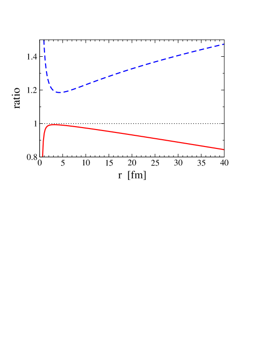
Figure 13: Ratios of the leading (dashed line) and next–to–leading order (solid line) HB potentials to the relativistic result versus the distance $r$ as explained in the text.

To see how the above qualitative arguments and estimations work in practice, we again follow Ref. [185] and calculate the leading and next–to–leading order HB approximations for the potential in coordinate space which correspond to the first and the first $+$ second terms in the series in Eq. (3.68). In Fig. 13 we show the ratios of these leading and next–to–leading order HB potentials to the relativistic result corresponding to the spectral function in Eq. (3.66). Here, we adopt the same values for the LECs $c_{1,3}$ as in section 3.2.1. As expected, the deviations from the correct result increase for large values of $r$. Notice that large deviations at short distances $r<1$ fm are due to the fact that the HB expansion diverges at large $\mu$. The leading HB approximation deviates by $\sim 20$% from the relativistic result in the region of physical interest. For further discussion of these and related issues, the reader is referred to [185].

To conclude, the formal inconsistency of the HB approach strongly affects the behavior of the potential at asymptotically large distances. In this region, however, the potential is very weak and its contribution to observables is negligible. At physically interesting distances, the effects due to the formal inconsistency of the HB expansion are small and expected to be irrelevant at the considered order. The 2PE potential has been derived at order $\nu=4$ in the relativistic version of chiral EFT [187, 188] using the formalism based on the S–matrix, see also Ref. [186] for the application to peripheral NN scattering.

3.3 Few–nucleon forces

Two–nucleon forces discussed above provide the most important contribution to the Hamilton operator. Three– and more–nucleon forces are suppressed compared to the two–nucleon ones (2NFs) by powers of $Q/\Lambda$ and thus appear as corrections. It is important to take these corrections into account in order to understand the properties of few–nucleon systems at the quantitative level. The strength of the chiral EFT approach is that it provides a framework to derive few–nucleon forces in a systematic way and fully consistent with the 2NF.

3.3.1 Three– and four–nucleon forces in the isospin limit

According to the power counting in Eq. (2.47), three– and four–nucleon forces (4NFs) start to contribute at order $\nu=2$, i.e. they are suppressed by a factor $(Q/\Lambda)^{2}$ compared to the leading 2NF. The leading 3NF contribution arises from tree diagrams constructed with the order $\Delta_{i}=0$ vertices, see graphs (a), (b) and (c) in Fig. 14. The leading 4NF is represented by the disconnected tree diagrams (d) and (e). As pointed out by Weinberg [113], graph (a) does not contribute at order $\nu=2$ due to an additional suppression factor $Q/m$. The origin of this suppression is easily understood in terms of “old–fashioned” time–ordered perturbation theory. Since graph (a) does not give rise to reducible topologies, its contribution to the 3NF is given by the sum of all possible time–ordered graphs, which build up the corresponding Feynman diagram. Since energy is conserved at each vertex of a Feynman graph, the time derivative, which enters the Weinberg–Tomozawa $\pi\pi NN$ vertex, yields a difference of nucleon kinetic energies which scales as $Q^{2}/m$ instead of $Q$.

Figure 14: Leading contributions to 3NF (graphs (a)–(c)) and 4NF (graphs (d) and (e)) at order $\nu=2$ that vanish. For notation see Fig. 7.

Figure 15: Time–ordered 2PE diagrams at order $\nu=2$. The first and second rows show all possible irreducible topologies, while the third row subsumes reducible topologies. Graphs resulting from the interchange of the vertex ordering at the middle nucleon line are not shown. For notation see Fig. 7.

The remaining graphs (b)–(e) in Fig. 14 lead to vanishing contributions to the nuclear force when the latter is defined within an energy–independent formulation such as the method of unitary transformation, see e.g. [189, 190, 132]. Consider, for example, the 2PE 3NF resulting from diagram (b) which can be obtained evaluating the corresponding matrix elements of the operators in Eq. (3.16). The first term in this expression gives rise to irreducible time–ordered graphs (i.e. the ones without purely nucleonic intermediate states) shown in Fig. 15 and defines the 3NF potential in the Tamm–Dancoff method, which can be expressed schematically as

$$-\left[\frac{4}{\omega_{1}(\omega_{1}+\omega_{2})\omega_{2}}+\frac{2}{\omega_{1}^{2}(\omega_{1}+\omega_{2})}+\frac{2}{(\omega_{1}+\omega_{2})\omega_{2}^{2}}\right]M=-2\frac{\omega_{1}+\omega_{2}}{\omega_{1}^{2}\omega_{2}^{2}}M~{},$$ (3.70)

where $\omega_{i}=k_{0}=\sqrt{\vec{k}\,^{2}+M_{\pi}^{2}}$ denotes the pion energy and we pulled out the common factor $M$ representing the spin, isospin and momentum structure, which is obviously the same for all graphs in Fig. 15. The remaining two terms in Eq. (3.16) are specific for the method of unitary transformation and correspond to reducible topologies shown in Fig. 15. We remind the reader that although these diagrams contain purely nucleonic intermediate states, their contributions are not enhanced in the limit $m\to\infty$ and cannot be identified with the iteration of the potential in the dynamical equation. These diagrams are thus not truly reducible in the sense of “old–fashioned” time–ordered perturbation theory. The resulting contribution to the potential reads:

$$\left[\frac{2}{\omega_{1}^{2}\omega_{2}}+\frac{2}{\omega_{1}\omega_{2}^{2}}\right]M=2\frac{\omega_{1}+\omega_{2}}{\omega_{1}^{2}\omega_{2}^{2}}M~{}.$$ (3.71)

The cancellation between irreducible and reducible diagrams in the method of unitary transformation is now evident. The same sort of cancellation occures for the remaining graphs (c)–(e) in Fig. 14. In other words, the entire contribution to the scattering amplitude represented by the Feynman diagrams (b)–(e) in Fig. 14 is reproduced by iteration of the leading 2NF in the corresponding dynamical equation with no need to introduce additional few–nucleon forces. We therefore conclude that the 3NF and 4NF at order $\nu=2$ vanish completely.

Figure 16: Three–nucleon force at order $\nu=3$. For notation see Fig. 7.

The first non–vanishing 3NF contribution appears at order $\nu=3$, i.e. at N²LO, and arises from diagrams shown in Fig. 16. The contribution from graph (a) in this figure is given (in the 3N CMS) by [192]:

$$V^{\rm(3)}_{\rm 2\pi}=\sum_{i\not=j\not=k}\frac{1}{2}\left(\frac{g_{A}}{2F_{\pi}}\right)^{2}\frac{(\vec{\sigma}_{i}\cdot\vec{q}_{i})(\vec{\sigma}_{j}\cdot\vec{q}_{j})}{(\vec{q}_{i}\,^{2}+M_{\pi}^{2})(\vec{q}_{j}\,^{2}+M_{\pi}^{2})}F^{\alpha\beta}_{ijk}\tau_{i}^{\alpha}\tau_{j}^{\beta}\,,$$ (3.72)

where $\vec{q}_{i}\equiv\vec{p}_{i}\,^{\prime}-\vec{p}_{i}$; $\vec{p}_{i}$ ($\vec{p}_{i}\,^{\prime}$) is the initial (final) momentum of the nucleon $i$ and

$$F^{\alpha\beta}_{ijk}=\delta^{\alpha\beta}\left[-\frac{4c_{1}M_{\pi}^{2}}{F_{\pi}^{2}}+\frac{2c_{3}}{F_{\pi}^{2}}\vec{q}_{i}\cdot\vec{q}_{j}\right]+\sum_{\gamma}\frac{c_{4}}{F_{\pi}^{2}}\epsilon^{\alpha\beta\gamma}\tau_{k}^{\gamma}\vec{\sigma}_{k}\cdot[\vec{q}_{i}\times\vec{q}_{j}]\,.$$

The subscripts of the Pauli spin and isospin matrices refer to nucleon labels. The form (3.72) was shown to match with the low–momentum expansion of various existing phenomenological 3NFs provided they respect chiral symmetry. This issue is extensively discussed in [193]. The contributions from the remaining graphs (b) and (c) in Fig. 16 take the form [192, 194]

$$V^{\rm(3)}_{1\pi,\;\rm cont}=-\sum_{i\not=j\not=k}\frac{g_{A}}{8F_{\pi}^{2}}\,D\,\frac{\vec{\sigma}_{j}\cdot\vec{q}_{j}}{\vec{q}_{j}\,^{2}+M_{\pi}^{2}}\,\left(\mbox{\boldmath$\tau$}_{i}\cdot\mbox{\boldmath$\tau$}_{j}\right)(\vec{\sigma}_{i}\cdot\vec{q}_{j})\,,\quad\quad\quad V^{\rm(3)}_{\rm cont}=\frac{1}{2}\sum_{j\not=k}E\,(\mbox{\boldmath$\tau$}_{j}\cdot\mbox{\boldmath$\tau$}_{k})\,,$$ (3.73)

where $D$ and $E$ are the corresponding LECs from the Lagrangian of order $\Delta=1$. We stress that the proper incorporation of the Pauli principle allows to substantially reduce the number of independent operators yielding only two terms in Eq. (3.73) [194]. Notice further that no 4NFs appear at order $\nu=3$.

The first corrections to the 3NF as well as the first contribution to the 4NF arise at order $\nu=4$. Some examples of diagrams which contribute at this order are shown in Fig. 17. For the 3NF, one has to take into account all possible one–loop graphs constructed with the lowest–order vertices and tree diagrams with one insertion of the order $\Delta_{i}=2$ vertices. In addition, one has to include the leading $1/m$–corrections to diagrams (a)–(c) in Fig. 14. The leading contributions to the 4NF arise at order $\nu=4$ from connected tree diagrams with the lowest–order vertices. One should also consider various disconnected diagrams which might, in principle, also contribute to the 4NF at this order. Work along these lines is underway. The leading $1/m$–corrections to the static 2PE 3NF were already evaluated and can be found in Ref. [140]. The relative importance of various isospin–invariant contributions to few–nucleon forces discussed in this section and in sections 3.2.2, 3.2.3 and 3.2.4 are summarized in Table 1 based on the chiral power counting in Eq. (2.47). We stress that these results rely on the energy–independent formulation.

Figure 17: Examples of the three– and four–nucleon force contributions at order $\nu=4$. For notation see Figs. 7.

Chiral order	2N force	3N force	4N force
$\nu=0$	$V_{1\pi}+V_{\rm cont}$	$-$	$-$
$\nu=1$	$-$	$-$	$-$
$\nu=2$	$V_{1\pi}+V_{2\pi}+V_{\rm cont}$	$-$	$-$
$\nu=3$	$V_{1\pi}+V_{2\pi}$	$V_{2\pi}+V_{1\pi,\;\rm cont}+V_{\rm cont}$	$-$
$\nu=4$	$V_{1\pi}+V_{2\pi}+V_{3\pi}+V_{\rm cont}$	work in progress	work in progress

Table 1: Isospin–symmetric nuclear forces up to order $\nu=4$.

3.3.2 Isospin–breaking corrections

Let us now discuss isospin–breaking corrections to the 3NF which were recently worked out up to the same order $\nu=5$ as the corresponding 2NFs. No isospin–breaking four– and more nucleon forces appear up to this order. Similar to the 2NF, it is useful to classify the 3NF with respect to its isospin structure. Following the lines of Ref. [195], one distinguishes between the following three classes:

$$\begin{array}[]{lcl}\mbox{Class I:}&\mbox{\hskip 8.5359pt}&V_{\rm I}=\sum_{i\neq j\neq k}\left(\alpha_{I}^{ijk}+\beta^{ijk}_{I}\,\mbox{\boldmath$\tau$}_{i}\cdot\mbox{\boldmath$\tau$}_{j}+\gamma^{ijk}_{I}\left[\mbox{\boldmath$\tau$}_{i}\times\mbox{\boldmath$\tau$}_{j}\right]\cdot\mbox{\boldmath$\tau$}_{k}\right)\,,\\[2.58334pt] \mbox{Class II:}&&V_{II}=\sum_{i\neq j\neq k}\left(\alpha^{ijk}_{II}\,\tau^{3}_{i}\tau^{3}_{j}+\beta^{ijk}_{II}\,[\mbox{\boldmath$\tau$}_{i}\times\mbox{\boldmath$\tau$}_{j}]^{3}\tau^{3}_{k}\right)\,,\\[2.58334pt] \mbox{Class III:}&&V_{III}=\sum_{i\neq j\neq k}\left(\alpha_{III}^{ijk}\,\tau^{3}_{i}+\beta^{ijk}_{III}\,[\mbox{\boldmath$\tau$}_{i}\times\mbox{\boldmath$\tau$}_{j}]^{3}+\gamma^{ijk}_{III}\,\tau^{3}_{i}\,\mbox{\boldmath$\tau$}_{j}\cdot\mbox{\boldmath$\tau$}_{k}+\kappa_{III}^{ijk}\,\tau^{3}_{i}\,\tau^{3}_{j}\,\tau^{3}_{k}\right)\,,\end{array}$$ (3.74)

where $\alpha$, $\beta$, $\gamma$ and $\kappa$ are space and spin operators and the indices $i$, $j$, $k$ refer to the nucleon labels. The class (I) forces are isospin invariant while the class (II) 3NFs break isospin but respect charge symmetry. Finally, the class (III) forces are charge–symmetry–breaking. Contrary to the commonly used classification scheme in the 2N sector, see Eq. (3.48), conservation of the operator $\mbox{\boldmath$T$}^{2}$ with $T$ being the total isospin operator, which ensures that there is no isospin mixing, is not used in Eq. (3.74). This is because this property depends on the number of particles in the system under consideration. For example, all isospin–breaking two–nucleon forces, which do not cause isospin mixing in the two–nucleon system, lead to isospin mixing in the three–nucleon system.

The leading and subleading isospin–violating 3NFs arise at orders $\nu=4$ and $\nu=5$ from diagrams shown in Fig. 18 [195, 196, 197]. Graphs (a)–(c) result from a single insertion of the proton–to–neutron mass difference into the order $\nu=2$ 3NF diagrams shown in Fig. 14.

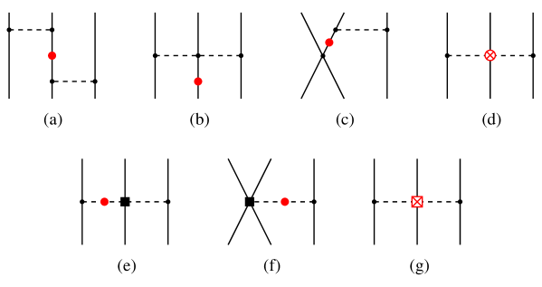
Figure 18: Isospin–breaking 3NF at orders $\nu=4$ (graphs (a)–(d)) and $\nu=5$ (graphs (e)–(g)). Graphs resulting by the interchange of the vertex ordering are not shown. For remaining notation see Figs. 7, 11 and 12.

Contrary to the corresponding isospin–invariant contributions discussed in section 3.3.1, diagrams (a)–(c) in Fig. 18 yield nonvanishing 3NFs. The origin of this difference is explained in detail in Ref. [125]. One finds the following class (III) 3NFs resulting from diagrams (a) and (c):

$$V^{\rm(4)}_{2\pi} = \sum_{i\not=j\not=k}\,2\delta m\,\left(\frac{g_{A}}{2F_{\pi}}\right)^{4}\frac{(\vec{\sigma}_{i}\cdot\vec{q}_{i})(\vec{\sigma}_{j}\cdot\vec{q}_{j})}{(\vec{q}_{i}{}^{2}+M_{\pi}^{2})^{2}(\vec{q}_{j}{}^{2}+M_{\pi}^{2})}\bigg{\{}[\vec{q}_{i}\times\vec{q}_{j}]\cdot\vec{\sigma}_{k}\,[\mbox{\boldmath$\tau$}_{i}\times\mbox{\boldmath$\tau$}_{j}]^{3}$$

$${}+\vec{q}_{i}\cdot\vec{q}_{j}\left[(\mbox{\boldmath$\tau$}_{i}\cdot\mbox{\boldmath$\tau$}_{k})\tau_{j}^{3}-(\mbox{\boldmath$\tau$}_{i}\cdot\mbox{\boldmath$\tau$}_{j})\tau_{k}^{3}\right]\bigg{\}}\,,$$

$$V^{\rm(4)}_{1\pi,\;\rm cont} = \sum_{i\not=j\not=k}2\,\delta m\,C_{T}\left(\frac{g_{A}}{2F_{\pi}}\right)^{2}\frac{\vec{\sigma}_{i}\cdot\vec{q}_{i}}{(\vec{q}_{i}{}^{2}+M_{\pi}^{2})^{2}}\,[\mbox{\boldmath$\tau$}_{k}\times\mbox{\boldmath$\tau$}_{i}]^{3}\;[\vec{\sigma}_{j}\times\vec{\sigma}_{k}]\cdot\vec{q}_{i}\,.$$ (3.75)

The contributions from the $2\pi$–exchange diagram (b) can naturally be combined with the contributions from graphs (d) and (g), which have the same structure. The resulting 3NF reads:

$$V_{2\pi}^{\rm(4,5)}=\sum_{i\not=j\not=k}\bigg{(}\frac{g_{A}}{2F_{\pi}}\bigg{)}^{2}\,\frac{(\vec{\sigma}_{i}\cdot\vec{q}_{i})(\vec{\sigma}_{j}\cdot\vec{q}_{j})}{(\vec{q}_{i}{}^{2}+M_{\pi}^{2})(\vec{q}_{j}{}^{2}+M_{\pi}^{2})}\,\Bigg{[}\frac{(\delta m)^{\rm str}}{4F_{\pi}^{2}}\Big{(}2(\mbox{\boldmath$\tau$}_{i}\cdot\mbox{\boldmath$\tau$}_{k})\tau_{j}^{3}-(\mbox{\boldmath$\tau$}_{i}\cdot\mbox{\boldmath$\tau$}_{j})\tau_{k}^{3}\Big{)}+f_{1}e^{2}\tau_{i}^{3}\tau_{j}^{3}\Bigg{]}\,.$$ (3.76)

While the term $\propto(\delta m)^{\rm str}$ breaks charge–symmetry, the contribution proportional to the LEC $f_{1}$ and arising from diagram (g) is charge–symmetry conserving, i.e. class (II). Isospin–violating $\pi\pi NN$ vertex $\propto f_{1}$ plays an important role in the analysis of isospin violation in pion–nucleon scattering [120] and the evaluation of the ground state characteristics of pionic hydrogen [124]. In the 2N sector, it only leads to an isospin–invariant contribution to the 2PE potential, which has the same form as the $c_{1}$–term in Eq. (3.2.2). The charge–symmetry–breaking part of $V_{2\pi}^{\rm(4,5)}$ in Eq. (3.76) was also obtained by Friar et al. [197] using a completely different approach. In their method, the neutron–to–proton mass difference, which is inconvenient to handle in practical calculations, is replaced by a series of new isospin–breaking vertices in the Lagrangian via an appropriate field redefinition, see Ref. [175] for more details. Finally, diagrams (e) and (f) due to the pion mass difference lead to the following class (II) 3NF at order $\nu=5$:

$$V^{\rm(5)}_{2\pi} = \sum_{i\not=j\not=k}\,\delta M_{\pi}^{2}\,\left(\frac{g_{A}}{2F_{\pi}}\right)^{2}\frac{(\vec{\sigma}_{i}\cdot\vec{q}_{i})(\vec{\sigma}_{j}\cdot\vec{q}_{j})}{(\vec{q}_{i}{}^{2}+M_{\pi}^{2})^{2}(\vec{q}_{j}{}^{2}+M_{\pi}^{2})}\Bigg{\{}\tau_{i}^{3}\tau_{j}^{3}\left[-\frac{4c_{1}M_{\pi}^{2}}{F_{\pi}^{2}}+\frac{2c_{3}}{F_{\pi}^{2}}(\vec{q}_{i}\cdot\vec{q}_{j})\right]$$

$$\mbox{\hskip 48.36958pt}+\frac{c_{4}}{F_{\pi}^{2}}\,\tau_{i}^{3}\,[\mbox{\boldmath$\tau$}_{j}\times\mbox{\boldmath$\tau$}_{k}]^{3}\,[\vec{q}_{i}\times\vec{q}_{j}]\cdot\vec{\sigma}_{k}\Bigg{\}}\,,$$

$$V^{\rm(5)}_{1\pi,\;\rm cont} = -\sum_{i\not=j\not=k}\,\delta M_{\pi}^{2}\,\frac{g_{A}}{8F_{\pi}^{2}}\,D\,\frac{\vec{\sigma}_{i}\cdot\vec{q}_{i}}{(\vec{q}_{i}{}^{2}+M_{\pi}^{2})^{2}}\,\tau_{i}^{3}\tau_{j}^{3}(\vec{\sigma}_{j}\cdot\vec{q}_{i})\,.$$ (3.77)

These results are consistent with the isospin–invariant 3NFs $V^{\rm(3)}_{\rm 2\pi}$ and $V^{\rm(3)}_{\rm 1\pi,\;cont}$ in Eqs. (3.72), (3.73) being expressed in terms of the charged pion mass. The corresponding expressions in coordinate space can be found in Ref. [195].

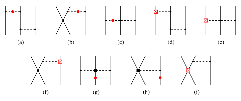
Figure 19: Leading (a–c) and subleading (d–i) isospin–violating contribution to the 3NF which vanish, as discussed in the text. Graphs resulting from the interchange of the vertex ordering are not shown. For notation see Figs. 7, 11 and 12.

In addition to graphs shown in Fig. 18, diagrams (a)–(c) and (d)–(i) in Fig. 19 formally contribute to the leading ($\nu=4$) and subleading ($\nu=5$) isospin–breaking 3NF, respectively. Their pertinent contributions, however, vanish. In particular, for graphs (a), (b), (d), (f) and (i) one observes the same sort of cancellation between various time orderings as in the case of the corresponding isospin–invariant 3NFs, see section 3.3.1 for more details. The contributions of diagrams (c) and (e) are suppressed by a factor of $Q/m$ due to the time derivative entering the Weinberg–Tomozawa vertex. Explicit evaluation of the remaining contributions of graphs (g) and (h) can be performed along the lines of ref. [195] and yields vanishing result.

Finally, we point out that there are many $1/m$–corrections to the obtained results which start to contribute at order $\nu=6$. Notice, however, that if one would adopt the counting rule $m\sim\Lambda$, various $1/m$–corrections (including the ones due to virtual photons) would contribute already at order $(Q/\Lambda)^{5}$. Some 3NF diagrams due to virtual photon exchange were considered by Yang and found to provide relatively small contributions of the order of $\sim 7$ keV to the ³He–³H binding–energy difference [198, 199]. Furthermore, we remind the reader that the long–range electromagnetic 3NFs might, potentially, cause large effects in scattering at low energy. The relative sizes of various isospin–breaking contributions to the two– and three–nucleon forces discussed in this section and in section 3.2.5 are summarized in Table 2. We stress that these results rely on the energy–independent formulation and on the counting rules specified in Eqs. (2.49), (3.46) and (3.47).

Chiral order		2N force			3N force
$\nu=0$		$-$			$-$
$\nu=1$		$-$			$-$
$\nu=2$		$V_{1\gamma}+V_{1\pi}$			$-$
$\nu=3$		$V_{1\pi}+V_{\rm cont}$			$-$
$\nu=4$		$V_{\pi\gamma}+V_{1\pi}+V_{2\pi}+V_{\rm cont}$			$V_{2\pi}+V_{1\pi,\;\rm cont}$
$\nu=5$		$V_{1\pi}+V_{2\pi}+V_{\rm cont}$			$V_{2\pi}+V_{1\pi,\;\rm cont}$

Table 2: Isospin–breaking two– and three–nucleon forces up to order $\nu=5$.

3.4 Role of the $\Delta$–excitation

The $\Delta$–isobar is well known to play an important role in hadronic and nuclear physics. This is due to its low excitation energy, $\Delta m\equiv m_{\Delta}-m=293$ MeV, and strong coupling to the $\pi N$ system. Because of the small value of $\Delta m$, it is not clear a priori whether in EFT it should be included explicitly, treating $\Delta m$ as a small quantity [200], or integrated out. On the one hand, inclusion of $\Delta$ yields a scheme, which differs from the chiral expansion since $\Delta m$ does not vanish in the chiral limit. On the other hand, it might provide a useful phenomenological extension and a systematic power counting has already been worked out assuming $\Delta m\sim M_{\pi}$ [201], see also [202] for an alternative scheme. In the chiral EFT discussed so far, the effects of the $\Delta$’s are only taken into account implicitly, i.e. through the values of the corresponding LECs [203]. We will now discuss the implications of treating the $\Delta$ as a dynamical degree of freedom in the EFT.

The leading contributions to the nuclear force due to the $\Delta$–excitation can be obtained in the heavy–baryon approach from the following terms in the Lagrangian [119, 201]

$$\mathcal{L}=\Delta^{\dagger}\left(i\partial_{0}-\Delta m\right)\Delta+\frac{h_{A}}{2F_{\pi}}\left(N^{\dagger}\vec{S}\mbox{\boldmath$T$}\Delta+\mbox{h.~{}c.}\right)\cdot\vec{\nabla}\mbox{\boldmath$\pi$}-D_{T}N^{\dagger}\vec{\sigma}\mbox{\boldmath$\tau$}N\cdot\left(N^{\dagger}\vec{S}\mbox{\boldmath$T$}\Delta+\mbox{h.~{}c.}\right)\,,$$ (3.78)

where $h_{A}$ and $D_{T}$ are LECs and $\Delta$ is a four–component spinor in both spin and isospin spaces that represents the delta. Further, $S_{i}$ ($T_{a}$) are the $2\times 4$ spin (isospin) transition matrices which satisfy the relations $S_{i}S_{j}^{\dagger}=(2\delta_{ij}-i\epsilon_{ijk}\sigma_{k})/3$ ($T_{a}T_{b}^{\dagger}=(2\delta_{ab}-i\epsilon_{abc}\tau_{c})/3$) [204]. Throughout this section, we will assume exact isospin symmetry. Notice that the large mass scale $m_{\Delta}$ disappears from the Lagrangian after performing the heavy–baryon expansion. Only the small scale $\Delta m$ enters the resulting Lagrangian.

The leading contributions to the 2NF due to intermediate $\Delta$ excitations arise at NLO, $\nu=2$, and are shown in Fig. 20.

Figure 20: Leading contributions to the $2\pi$–exchange potential with single and double $\Delta$–excitations. Double lines represent the $\Delta$–isobar. For remaining notation see Fig. 7.

In the context of chiral EFT, they were first discussed by Ordóñez et al. [119] based on “old–fashioned” time–ordered perturbation theory. These contributions were reconsidered by Kaiser et al. [205] using the Feynman graph technique. For completeness, we collect here the expressions for the corresponding non–polynomial pieces of the 2PE potential from [205] (generalized to SFR with arbitrary $\tilde{\Lambda}$) for the three distinct groups of terms:

• $\Delta$–excitation in the triangle graphs:

  $$V^{\rm 2\pi}_{\Delta,\,{\rm triangle}}=-\frac{h_{A}^{2}}{864\pi^{2}F_{\pi}^{4}}\,(\mbox{\boldmath$\tau$}_{1}\cdot\mbox{\boldmath$\tau$}_{2})\,\biggl{\{}(6E-\omega^{2})L^{\tilde{\Lambda}}(q)+12(\Delta m)^{2}ED^{\tilde{\Lambda}}(q)\biggr{\}}~{},$$ (3.79)

  with

  $$D^{\tilde{\Lambda}}(q)=\frac{1}{\Delta m}\,\int_{2M_{\pi}}^{\tilde{\Lambda}}\frac{d\mu}{\mu^{2}+q^{2}}\,\arctan\frac{\sqrt{\mu^{2}-4M_{\pi}^{2}}}{2\Delta m}~{},\quad\quad E=2M_{\pi}^{2}+q^{2}-2(\Delta m)^{2}~{}.$$ (3.80)

• Single $\Delta$–excitation in the box graphs:

  $$V^{\rm 2\pi}_{\Delta,\,{\rm box}-1} = -\frac{g_{A}^{2}\,h_{A}^{2}}{48\pi F_{\pi}^{4}\Delta m}\,(2M_{\pi}^{2}+q^{2})^{2}\,A^{\tilde{\Lambda}}(q)$$ (3.81)

  $$- \frac{g_{A}^{2}\,h_{A}^{2}}{864\pi^{2}F_{\pi}^{4}}\,(\mbox{\boldmath$\tau$}_{1}\cdot\mbox{\boldmath$\tau$}_{2})\,\biggl{\{}(12(\Delta m)^{2}-20M_{\pi}^{2}-11q^{2})L^{\tilde{\Lambda}}(q)+6E^{2}D^{\tilde{\Lambda}}(q)\biggr{\}}$$

  $$- \frac{g_{A}^{2}\,h_{A}^{2}}{192\pi^{2}F_{\pi}^{4}}\,\biggl{(}(\vec{\sigma}_{1}\cdot\vec{q}\,)(\vec{\sigma}_{2}\cdot\vec{q}\,)-q^{2}(\vec{\sigma}_{1}\cdot\vec{\sigma}_{2})\biggr{)}\,\biggl{\{}-2L^{\tilde{\Lambda}}(q)+(\omega^{2}-4(\Delta m)^{2})D^{\tilde{\Lambda}}(q)\biggr{\}}$$

  $$- \frac{g_{A}^{2}\,h_{A}^{2}}{576\pi F_{\pi}^{4}\Delta m}\,(\mbox{\boldmath$\tau$}_{1}\cdot\mbox{\boldmath$\tau$}_{2})\,\biggl{(}(\vec{\sigma}_{1}\cdot\vec{q}\,)(\vec{\sigma}_{2}\cdot\vec{q}\,)-q^{2}(\vec{\sigma}_{1}\cdot\vec{\sigma}_{2})\biggr{)}\,\omega^{2}\,A^{\tilde{\Lambda}}(q)~{}.$$

• Double $\Delta$–excitation in the box graphs:

  $$V^{\rm 2\pi}_{\Delta,\,{\rm box}-2} = -\frac{h_{A}^{4}}{432\pi^{2}F_{\pi}^{4}}\,\biggl{\{}-4(\Delta m)^{2}L^{\tilde{\Lambda}}(q)+E[H^{\tilde{\Lambda}}(q)+(E+8(\Delta m)^{2})D^{\tilde{\Lambda}}(q)]\biggr{\}}$$

  $$- \frac{h_{A}^{4}}{7776\pi^{2}F_{\pi}^{4}}\,(\mbox{\boldmath$\tau$}_{1}\cdot\mbox{\boldmath$\tau$}_{2})\,\biggl{\{}(12E-\omega^{2})L^{\tilde{\Lambda}}(q)+3E[H^{\tilde{\Lambda}}(q)+(8(\Delta m)^{2}-E)D^{\tilde{\Lambda}}(q)]\biggr{\}}$$

  $$- \frac{h_{A}^{4}}{3456\pi^{2}F_{\pi}^{4}}\,\biggl{(}(\vec{\sigma}_{1}\cdot\vec{q}\,)(\vec{\sigma}_{2}\cdot\vec{q}\,)-q^{2}(\vec{\sigma}_{1}\cdot\vec{\sigma}_{2})\biggr{)}\,\biggl{\{}6L^{\tilde{\Lambda}}(q)+(12(\Delta m)^{2}-\omega^{2})D^{\tilde{\Lambda}}(q)\biggr{\}}$$

  $$- \frac{h_{A}^{4}\,(\mbox{\boldmath$\tau$}_{1}\cdot\mbox{\boldmath$\tau$}_{2})}{20736\pi^{2}F_{\pi}^{4}}\,\biggl{(}(\vec{\sigma}_{1}\cdot\vec{q}\,)(\vec{\sigma}_{2}\cdot\vec{q}\,)-q^{2}(\vec{\sigma}_{1}\cdot\vec{\sigma}_{2})\biggr{)}\,\biggl{\{}2L^{\tilde{\Lambda}}(q)+(4(\Delta m)^{2}+\omega^{2})D^{\tilde{\Lambda}}(q)\biggr{\}}~{},$$

  with

  $$H^{\tilde{\Lambda}}(q)=\frac{2E}{\omega^{2}-4(\Delta m)^{2}}\biggl{[}L^{\tilde{\Lambda}}(q)-L^{\tilde{\Lambda}}(2\sqrt{(\Delta m)^{2}-M_{\pi}^{2}})\biggr{]}\quad.$$ (3.83)

Notice that some of the above contributions, in particular, those ones corresponding to the first and the last lines in Eq. (3.81), have precisely the same structure as the corresponding N²LO terms in EFT without $\Delta$’s, see Eq. (3.2.2) provided one chooses

$$-c_{3}=2c_{4}=\frac{h_{A}^{2}}{9\Delta m}\,.$$ (3.84)

Using the large–$N_{c}$ value $h_{A}=3g_{A}/\sqrt{2}$ and comparing the LECs in Eq. (3.84) with the ones in EFT without explicit $\Delta$’s [154], one concludes that the $\Delta$ provides the dominant (significant) contribution to $c_{3}$ ($c_{4}$). Resonance saturation for these and other $\pi N$ LECs is discussed in detail in [203]. The remaining contributions to the NN potential due to intermediate $\Delta$–excitation in Eqs. (3.79)–(• ‣ 3.4) show a non–trivial dependence on the $N\Delta$ mass splitting. We further emphasize that some of the subleading corrections to the 2PE potential with intermediate $\Delta$–excitations are discussed in [119] while the leading relativistic corrections of order $\nu=4$ can be found in [205].

Let us now switch to the leading 3NF contributions due to intermediate $\Delta$ excitations, which also arise at NLO and are shown in Fig. 21.

Figure 21: Leading contributions to the 3NF due to explicit $\Delta$’s. For notation see Figs. 7 and 20.

In the context of chiral EFT, they were first discussed in Ref. [192]. We remind the reader that in the EFT without explicit $\Delta$’s, the first nonvanishing contribution to the 3NF in the energy independent formulation only arises at N²LO, $\nu=3$, see section 3.3.1. The 2PE contribution from the first graph in Fig. 21 has the same form as the corresponding terms in the theory without delta, see Eq. (3.72), provided one chooses $c_{1}=0$ and $c_{3,4}$ according to Eq. (3.84). Interestingly, the contributions of the two other diagrams in Fig. 21 vanish as a consequence of the Pauli principle, see [194] for a related discussion.

To summarize, the effects due to intermediate $\Delta$ excitations in the EFT with explicit $\Delta$’s first show up at NLO (NLO-$\Delta$). At this order, one finds important contributions to the 2PE 2N and 3N potentials. In the EFT without explicit $\Delta$’s, the major part of these terms is shifted to N²LO (N²LO-$\Delta/$) and represented by the contributions proportional to LECs $c_{3,4}$ which are saturated by the $\Delta$. In particular, the leading isoscalar central and isovector spin–spin and tensor components in Eq. (3.81) are exactly reproduced at N²LO-$\Delta/$. For the 3NF, the functional form of the NLO-$\Delta$ contribution is completely recovered at N²LO-$\Delta/\,$. We stress, however, that the strength of the 2PE 3NF at N²LO-$\Delta/$ is overestimated by a factor of 4/3 compared to the one at NLO-$\Delta$ if the values of the LECs $c_{3,4}$ are fixed from $\pi N$ scattering at threshold [206]. Clearly, higher–order counter terms remove this discrepancy.

Despite the fact that many of the NLO-$\Delta$ contributions to the nuclear force are reproduced at N²LO-$\Delta/$, it might be advantageous to treat the delta isobar as an explicit degree of freedom. This might help to increase the range of applicability of the EFT. Further, one expects that such an approach would lead to the contributions to the nuclear force of a more natural size. For example, the large portion of the 2PE potential $\propto c_{i}$ at N²LO-$\Delta/$, which is known to be very strong, is shifted to NLO in the EFT with explicit $\Delta$’s. Similar effects are also observed for isospin–breaking terms, see [195, 125]. We emphasize, however, that such an approach with explicit $\Delta$’s is much more complicated since one has to deal with more structures and also needs e.g. to reanalyze pion-nucleon scattering (see Ref. [207] for an attempt). For some recent related work in the single–nucleon sector the reader is referred to [208, 209, 210].

4 Applications to few–nucleon systems

4.1 The two–nucleon system

4.1.1 Peripheral nucleon–nucleon scattering

Nucleon–nucleon scattering in peripheral partial waves within the chiral EFT framework has attracted a special interest in the past few years [142, 211, 147, 212, 186], see also Ref. [213] for a related work. This has several reasons. First, the contribution of the short–range contact interactions is suppressed due to the centrifugal barrier in partial waves with large values of the orbital angular momentum. For example, no contact terms contribute to D– (F–) and higher partial waves up to N³LO (N⁵LO). Consequently, peripheral phase shifts are entirely determined by the long–range part of the nuclear force and thus are expected to provide a sensitive test of the chiral 2PE potential. Secondly, the smallness of the corresponding phase shifts suggests that they should be describable in perturbation theory. This allows one to avoid the additional complication related to the nonperturbative treatment of the Schrödinger equation. The validity of perturbation theory is confirmed by the conventional scenario of nuclear forces based on the existing boson–exchange models and various phenomenological potentials, see [214]. It should be understood that the weakness of the chiral NN force in peripheral channels, which justifies the use of perturbation theory, may only be verified assuming a particular regularization scheme for the chiral potential, which shows a singular behavior at the origin. Using, for example, dimensional regularization, the iterated 1PE potential was found to be numerically small in most peripheral channels [142]. Notice, however, that the weakness of the NN interaction for high values of $l$ is not related to the chiral expansion and does not follow from the chiral power counting. We further stress that the role of peripheral NN scattering and the resulting constraints on the values of the LECs should not be overestimated since the observables at low and moderate energies are, in general, only weakly affected by peripheral phase shifts.

We will now consider D– and higher partial waves up to N²LO in chiral EFT following the lines of Ref. [147]. Using Born approximation for the scattering amplitude, the phase shifts and mixing angles in the convention of Stapp et al. [215] are determined by the 2N potential as:

$$\delta^{sj}_{l}=-\frac{mq}{(4\pi)^{2}}\langle lsj|V_{\rm 2N}|lsj\rangle\,,\quad\quad\epsilon_{j}=-\frac{mq}{(4\pi)^{2}}\langle j-1,sj|V_{\rm 2N}|j+1,sj\rangle\,,$$ (4.1)

where $s$ and $j$ refer to the total spin and angular momentum, respectively, and $q$ is the nucleon CMS momentum. Clearly, such an approximation violates unitarity. This violation is small provided that the corresponding phase shifts are small. Alternatively, one can use the $K$–matrix approach in order to restore unitarity, see e.g. [211]. Here and in what follows, we adopt the same notation for the matrix elements in the $|lsj\rangle$ basis as in Ref. [162]. The formulae for the partial wave decomposition can be found in appendix B of this reference. Up to N²LO, the potential $V_{\rm 2N}$ consists of the $1\pi$–exchange and the leading and subleading $2\pi$–exchange terms given in Eqs. (3.32), (3.2.2) and (3.2.2), respectively. The contact interactions do not contribute to D–waves at this order. For the sake of simplicity, we neglect isopin–violating effects in this section. In what follows, we adopt the same values of the LECs as in [162]: $g_{A}=1.26$, $F_{\pi}=92.4$ MeV and $M_{\pi}=138.03$ MeV. For the Goldberger–Treiman discrepancy in Eq. (3.32), we use $\delta=0.03$, which leads to $g_{\pi N}\simeq 13.2$. In addition, we have to specify the values of the LEC $c_{1,3,4}$ which determine the strength of the subleading 2PE potential. Table 3 summarizes some of the modern determinations of these LECs, see also Ref. [216] where a different notation was used. We also include the LEC $c_{2}$ in Table 3, which first contributes to the potential at order $\nu=4$. For a precise meaning of the indicated errors in the various determinations, the reader is referred to the original publications. Presumably, the most reliable determination of the $c_{i}$’s from the $\pi N$ system in the third order HBCHPT is performed in Ref. [154]. In this work, the $\pi N$ scattering amplitude is reconstructed in the unphysical region using dispersion relations, where the chiral expansion is expected to converge rapidly. Unfortunately, this method does not allow for a reliable determination of $c_{2}$.

	Ref.	$c_{1}$	$c_{2}$	$c_{3}$	$c_{4}$
$\pi N$, $Q^{2}$	[217]	$-$0.64(14)	1.78(20)	$-$3.90(9)	2.25(9)
$\pi N$, $Q^{3}$	[203]	$-$0.93(10)	3.34(20)	$-$5.29(25)	3.63(10)
$\pi N$, $Q^{3}$ (fit 1)	[218]	$-$1.23(16)	3.28(23)	$-$5.94(9)	3.47(5)
$\pi N$, $Q^{3}$ (fit 1)	[154]	$-$0.81(15)	9.35(66.7)	$-$4.69(1.34)	3.40(4)
$NN$	[211]	$-$0.81⋆	3.28⋆	$-$3.40	3.40⋆
$pp$	[219]	$-$0.76⋆	–	$-$5.08(28)	4.70(70)
$NN$	[220]	$-$0.76⋆	–	$-$4.78(10)	3.96(22)

Table 3: Recent determinations of the LECs $c_{i}$. All values are in GeV^-1. The values of the LECs used as input are marked by the star.

Recently, the Nijmegen group incorporated the chiral 2PE potential up to order $\nu=3$ in an energy–dependent PWA of the $pp$ data [219] and $pp\,+\,np$ data [220] and was able to extract the values of the LECs $c_{3,4}$, see Table 3. The resulting LECs $c_{3,4}$ are consistent with the $Q^{3}$–determinations in the $\pi N$ system (with the value of $c_{4}$ being on the upper side). We stress that the errors indicated in these references are statistical. It is not fully clear how the complete theoretical uncertainty can be estimated in this approach, which is not entirely based on EFT, see also [221] for a related discussion. A somewhat smaller value of the LEC $c_{3}$, $c_{3}=-3.4$ GeV^-1, was found in Ref. [211] to be consistent with empirical NN phase shifts as well as the results from dispersion and conventional meson theories. In that work, F– and higher partial waves were studied in chiral EFT at order $\nu=4$. Notice that the phase shifts depend most sensitively on $c_{3}$ and are less sensitive on variations of $c_{1,2,4}$. Similar smaller values for $c_{3}$ were also found by Higa [186], who looked at peripheral NN waves in the relativistic version of chiral EFT at order $\nu=4$. Interestingly, similar values for the LEC $c_{3}$ were also extracted recently from matching the chiral expansion of the nucleon mass to lattice gauge theory results at pion masses between 500 and 800 MeV [152]. Given the present uncertainty in the value of $c_{3}$, we will show the results corresponding to the following two choices: the central value from [154], $c_{3}=-4.7$ GeV^-1, and the value from Ref. [211], $c_{3}=-3.4$ GeV^-1. For the LECs $c_{1,4}$ we adopt the central values from the $Q^{3}$–analysis of the $\pi N$ system [154]: $c_{1}=-0.81$ GeV^-1, $c_{4}=3.40$ GeV^-1.

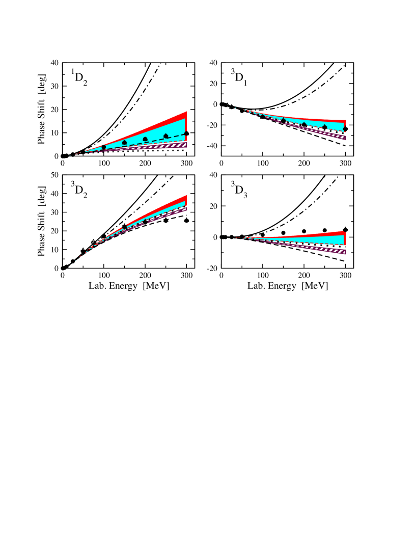
Figure 22: D–wave NN phase shifts. The dotted curve is the LO prediction (i.e. based on the pure 1PE potential). Dashed, dash–dotted and solid curves are the NLO, N²LO with $c_{3}=-3.4$ GeV^-1 and N²LO with $c_{3}=-4.7$ GeV^-1 results based on the DR potential. The dashed, light shaded and dark shaded bands refer to the NLO, N²LO with $c_{3}=-3.4$ GeV^-1 and N²LO with $c_{3}=-4.7$ GeV^-1 results using the SFR with $\tilde{\Lambda}=500\ldots 800$ MeV. The filled circles (open triangles) depict the results from the Nijmegen multi–energy PWA [108, 109] (Virginia Tech single–energy PWA [222]).

Let us begin with the D–waves which are shown in Fig. 22. The LO result represented by the pure 1PE potential already provides a good approximation to the phase shifts in the ${}^{3}D_{1}$ and ${}^{3}D_{2}$ partial waves. It is too weak in the ${}^{1}D_{2}$ channel and does not describe properly the ${}^{3}D_{3}$ phase shift. The latter one appears to be quite small ($|\delta|\sim 4.6^{\circ}$ at $E_{\rm lab}=300$ MeV) compared to the other D–wave phase shifts ($|\delta|\sim 9.7^{\circ}\ldots 25.5^{\circ}$). The reason is that the partial–wave projected 1PE, taken on the energy shell, is strongly suppressed in this channel. Consequently, the ${}^{3}D_{3}$ phase shift is sensitive to 2PE but also to the iteration of the potential which is neglected here. The NLO predictions show a visible improvement for the ${}^{1}D_{2}$ phase shift but go into the wrong direction in the ${}^{3}D_{1}$ and ${}^{3}D_{3}$ channels. The N²LO results based on DR are depicted by the dash–dotted and solid lines for the two choices of the LEC $c_{3}$ specified above. The reasonable agreement with the data observed at LO and NLO is destroyed in all partial waves for energies $E_{\rm lab}>50$ MeV and the chiral expansion does not seem to converge. Notice that similar deviations from the data are also observed for mixing angle $\epsilon_{2}$ which is not shown here [142, 147]. This disagreement with the data for the DR potential was first pointed out in [142] and then also reported in Ref. [147]. We stress that the results presented here are parameter–free. As pointed out by Kaiser et al. [142], the origin of the strong disagreement with the data can be traced back to the central part of the subleading 2PE potential, see Eq. (3.2.2), which is proportional to the LEC $c_{3}$ and shows an unphysically strong attraction at intermediate and short distances when DR is used to regularize the divergent integrals. This is demonstrated explicitly in Fig. 6, where the chiral potential is compared to phenomenological $\sigma$ ($\sigma+\omega+\rho$) contributions. Notice that another consequence of the strong attraction of the subleading 2PE potential is given by the unphysical bound states in low partial waves which could not be avoided in the N²LO analysis of Ref. [139]. Although such spurious bound states do not influence NN observables at low energies, they are at least inconvenient for the application to few–nucleon systems and might influence processes like e.g. Nd [214] or $\pi$d [223] scattering.

The strong attraction of the subleading 2PE potential can partially be explained by the large values of the LECs $c_{i}$. For example, the absolute value of the dimensionless coupling corresponding to the LEC $c_{3}$ is of the order $\sim 10$ which has to be compared with its expected natural size of the order $\sim 1$ [203]. The origin of this enhancement is well understood [203]: the LECs $c_{3,4}$ are, to a large extent, saturated by the $\Delta$–excitation. This implies that a new and smaller scale, namely $m_{\Delta}-m\sim 293$ MeV, enters these LECs in EFT without explicit $\Delta$, see also the discussion in section 3.4. As shown in Fig. 6, the large numerical value of $c_{3}$ appears to be consistent with the results based on phenomenological potential models at large distances, where the chiral potential is unaffected by the regularization procedure. On the other hand, the behavior of the 2PE potential at intermediate and short distances depends, to a large extent, on the way one regularizes the corresponding loop integrals, see section 3.2.1. The unphysically strong attraction of the 2PE potential in the region $r\lesssim 1/M_{\pi}\sim 1.4$ fm arises from high–momentum components of the exchanged pions, which cannot be properly treated in an EFT but whose contribution is, nevertheless, included in the potential obtained using DR. In the SFR approach, these high–momentum components in the mass spectrum are explicitly removed. As depicted in Fig. 6, using SFR with the reasonably chosen cut–off $\tilde{\Lambda}=500\ldots 800$ MeV greatly reduces this unphysical attraction and the resulting potential is of the same order in magnitude as the one obtained in phenomenological boson–exchange models. The results for D–waves are strongly improved using the spectral function regularization instead of dimensional one, as documented in Fig. 22. It should be understood that dimensional regularization is by no means ruled out by such consideration. In general, for quickly converging expansions, it can and should be the method of choice. If, however, the convergence for some well understood physical reason is slow and (some) observables become sensitive to spurious short–distance physics kept in DR, it is preferable to use SFR. Choosing DR, one picks up a portion of spurious short–distance physics which, under normal circumstances, can be compensated by the counter terms included in the potential at a given order. In the case at hand, however, unnaturally large counter terms (contact interactions) are required due to the large values of the LECs $c_{3,4}$. The neglect of higher–order contact terms is, therefore, not justified and results in a large disagreement with the data. It is known that a counter term at order $\nu=4$ is able to remove the bulk of the disagreement observed for D–waves in the DR based approach [139, 224, 163]. The unnaturally large size of the leading counter term in the ${}^{1}D_{2}$ partial wave was also found in Ref. [212] based on the distorted wave method. On the other hand, applying SFR with the cut–off $\tilde{\Lambda}$ of the order of the separation scale allows to remove the spurious short–range physics from the potential, which results in a more natural size of the counter terms. As demonstrated in Fig. 22, no N³LO counter terms need then to be taken into account at N²LO. In other words, the convergence of the chiral expansion is substantially improved using SFR with the reasonably chosen cut–off $\tilde{\Lambda}$ instead of DR. We refer the reader to Refs. [148, 149, 150] where a similar method has been applied to improve the convergence of the SU(3) baryon CHPT.

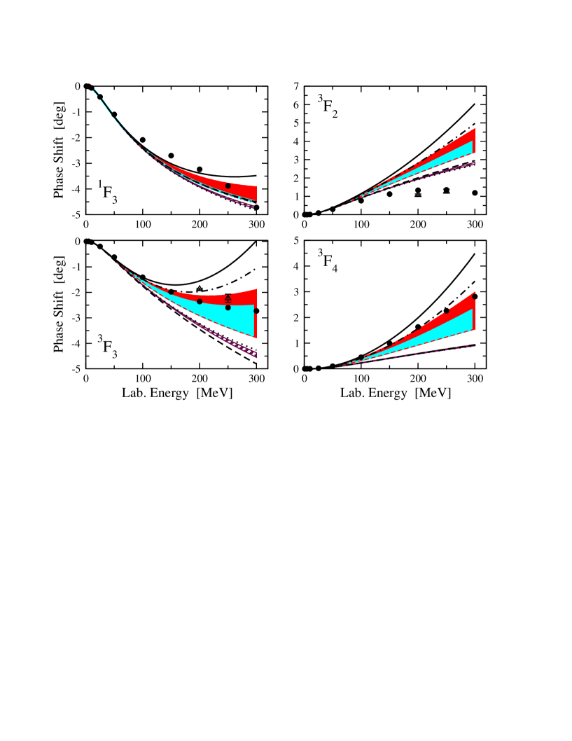
Figure 23: F–wave NN phase shifts. For notation see Fig. 22.

The results for F–waves are presented in Fig. 23. Although the situation with the DR subleading 2PE potential is much less dramatic compared to D–waves, a too strong attraction is clearly visible in the ${}^{3}F_{2}$, ${}^{3}F_{3}$ and ${}^{3}F_{4}$ partial waves, especially if one uses $c_{3}=-4.7$ GeV^-1, see also [142]. Removing the short–distance components of the 2PE potential with the cut–off regularization improves the results in the ${}^{3}F_{3}$ channel, while additional repulsion is still missing in the ${}^{3}F_{2}$ partial wave. A much smaller sensitivity of F–waves to the choice of regularization and thus to short–range physics is, of course, the consequence of the stronger centrifugal barrier. The leading contact terms in F–waves are suppressed by $(Q/\Lambda)^{2}$ compared to D–waves and appear first at order $\nu=6$. Therefore, even if the corresponding LECs are large in the approach based on DR, neglecting those terms leads to much smaller effects in F–waves.

The dependence of the phase shifts on the SFR cut–off being varied in a certain reasonable range reflects the influence of the higher–order contact terms and thus provides a natural estimation of the theoretical uncertainty at a given order. The typical uncertainty of $\sim 30$% observed in the N²LO predictions at $E_{\rm lab}=300$ MeV is consistent with the power counting, see [147] for more details. In view of this theoretical uncertainty, it appears to be impossible to make any preference in favor of the choice $c_{3}=-4.7$ GeV^-1 or $c_{3}=-3.4$ GeV^-1 based on the D– and F–waves at N²LO.

Let us now briefly summarize the main results for D– and F–waves at N²LO:

• The subleading 2PE potential obtained using DR leads to strong disagreement with the data in D–waves (F–waves) for $E_{\rm lab}\gtrsim 50$ MeV ($E_{\rm lab}\gtrsim 150$ MeV) and for both choices $c_{3}=-4.7$ GeV^-1 and $c_{3}=-3.4$ GeV^-1 (for the choice $c_{3}=-4.7$ GeV^-1).

• Using SFR instead of DR with the cut–off $\tilde{\Lambda}=500\ldots 800$ MeV strongly (sizably) improves the description of the phase shifts in D–waves (F–waves).

• The theoretical uncertainty in the description of D– and F–waves is sizable at large energy.

As already mentioned before, F– and higher NN phase shifts were also studied at order $\nu=4$ in both the standard heavy–baryon [211] and relativistic framework [186]. The authors of Ref. [211] use the perturbative approach similar to the one described above but also take into account the contribution of the once iterated 1PE potential and adopt a different counting rule for the nucleon mass ($m\sim\Lambda$). F–wave phase shifts obtained in this work and based on the choice $c_{3}=-3.4$ GeV^-1, are shown in Fig. 24. The results at LO, NLO and N²LO are similar to the ones shown in Fig. 23. The N³LO corrections are found to be small in the ${}^{1}F_{3}$ and ${}^{3}F_{4}$ channels and noticeable in the ${}^{3}F_{2}$ and ${}^{3}F_{3}$ partial waves, where they slightly increase the disagreement with the data. We will discuss NN phase shifts at order $\nu=4$ in more detail in section 4.1.3.

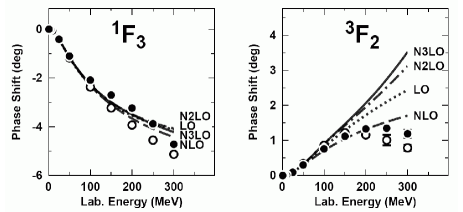
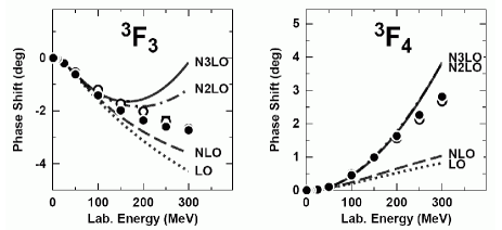
Figure 24: F–wave neutron–proton phase shifts from Ref. [211]. The solid dots and open circles are the results from Nijmegen PWA [108, 109] and Virginia Tech analysis SM99 [222]. Figure courtesy of Ruprecht Machleidt.

Last but not least, we would like to comment on an early attempt of Ref. [214] to avoid the above mentioned difficulties caused by the strong attraction of the subleading 2PE potential. In this work based on the DR version of the 2PE potential, smaller in magnitude values of the LECs $c_{3,4}$, namely $c_{3}=-1.15$ GeV^-1, $c_{4}=1.20$ GeV^-1, were adopted in order to reduce the unphysical attraction at N²LO. This allowed for a fairly good description of the NN data with no spurious bound states and enabled applications to few–nucleon systems, see e.g. [194]. Clearly, such an approach is still not satisfactory due to its incompatibility with $\pi$N scattering. The framework based on SFR allows to avoid the above mentioned difficulties and, at the same time, stay consistent with $\pi$N scattering. It should, therefore, be the method of choice. We will show some results based on the reduced $c_{3,4}$ from [214] in section 4.2.

4.1.2 Regularization and renormalization of the Schrödinger equation

In the previous section, we considered peripheral NN scattering in perturbation theory. To properly describe low partial waves, where the interaction is strong, the Lippmann–Schwinger (LS) equation for the scattering amplitude has to be solved nonperturbatively. The nuclear potential derived in chiral EFT is only valid for small momenta and becomes meaningless in the large–momentum region. The results presented in section 3.2 show that it grows with increasing momenta. Consequently, the LS equation is ultraviolet divergent and needs to be regularized (and renormalized). The problem of renormalization in the nonperturbative regime in the context of chiral EFT attracted a lot of interest in the past years, see e.g. [77, 225, 226, 227, 228, 229, 230, 231, 232, 233, 234, 235, 116, 117]. Here, one difficulty is due to the fact that the two–nucleon scattering amplitude can only be obtained numerically if pion–exchange contributions are treated nonperturbatively. In addition, since the nuclear potential is nonrenormalizable (in the traditional sense), an infinite number of counter terms is needed to remove all ultraviolet divergences generated by the iteration of the potential in the LS equation. Notice that this feature is in strong contrast to the pion and single–nucleon sectors as well as to the KSW approach discussed in section 2.3, where all divergences at a given order in the chiral expansion can be removed explicitly by a redefinition of a finite number of parameters in the Lagrangian. At first sight, this seems to be in contradiction with the power counting discussed in section 2.3, which tells us that a finite number of counter terms have to be included in the potential at any finite order in the chiral expansion. Moreover, the infinite number of counter terms needed to remove all divergences in the LS equation raises the question, whether the EFT in the 2N sector still has predictive power. Fortunately, this indeed appears to be the case. We recall that the power counting outlined in section 2.3 is formulated for renormalized contributions to the amplitude. Provided that the renormalized LECs are of natural size as explained in section 2.3, the contribution of higher–order counter terms is suppressed by powers of the low momentum scale $Q$ and thus does not need to be taken into account.

The standard procedure to renormalize the LS equation is based on Wilson’s method [236] and implies the following two steps. First, one solves the LS equation regularized with the finite momentum (or coordinate space) cut–off and with the kernel represented by the potential truncated at a given order in the chiral expansion. Secondly, the LECs, which accompany the short–range contact interactions entering the potential, are determined by matching the resulting phase shifts to experimental data. Based on the “naive dimensional analysis”, see e.g. [94], one expects the resulting LECs to be of natural size. The contributions of the neglected higher–order terms in the potential are expected to be small and irrelevant at the considered order. Notice that the exact form of the regulator used in the LS equation is irrelevant (provided it does not affect the long–distance behavior of the potential). There is a certain freedom in choosing the value of the cut–off. For the sake of definiteness, let us consider the momentum space cut–off $\Lambda$. It is clear that taking a too small $\Lambda$ will remove the truly long–distance physics and reduce the predictive power of the EFT. On the other hand, as argued in [238, 237, 94], taking too large values of $\Lambda$ leads to a highly nonlinear behavior and should be avoided as well. An example of such a nonlinear behavior is given by the appearance and accumulation of bound states for regularized $1/r^{n}$ attractive singular potentials. In this case, the renormalization–group behavior of the LECs appears to be of a limit cycle type (this feature depends on the regularization employed [88]), so that the “naive dimensional analysis” is not applicable anymore, see Ref. [116] for a recent related discussion. This example is also of relevance for the 1PE potential, whose tensor component behaves at short distances as $1/r^{3}$. Taking the limit $\Lambda\to\infty$ in the LS equation will, therefore, generate bound states in partial waves with arbitrarily high values of the orbital angular momentum $l$ and lead to strong deviations from the data. As a consequence, an infinite number of higher–order counter terms will be needed in this limit in order to restore the agreement with the data. This problem is, clearly, an artifact of the unphysical behavior of the point–like static 1PE potential at large momenta (or short–distances). In this region, the chiral expansion is not applicable, and the 1PE potential does not properly describe the true interaction between the nucleons. Using a finite cut–off $\Lambda$ of the order of the characteristic hard scale of the theory allows to avoid this problem in a natural way. It should also be understood that no improvement in the description of the data can, in general, be expected increasing $\Lambda$ beyond the pertinent hard scale unless new physics corresponding to this scale is properly incorporated in the theory. For a much more extensive discussion of these issues including many explicit examples, the reader is referred to [237, 238, 94], see also [116, 117] for a recent related work.

Let us further mention that the consistency of Weinberg’s approach has been questioned in Refs. [75, 76], where it was pointed out, based on perturbative arguments, that the order $\nu=2$ contact term $\propto M_{\pi}^{2}$ needs to be taken into account in order to absorb the ultraviolet divergence generated by the iteration of the order $\nu=0$ potential. This problem with the formal inconsistency of the Weinberg scheme was also addressed in Ref. [114] based on a nonperturbative approach and found to be present in the ${}^{1}S_{0}$–channel while absent in the coupled ${}^{3}S_{1}$–${}^{3}D_{1}$–channel. In that work, a new power counting scheme was invented based on the expansion of the potential about the chiral limit, see [114] for more details. It remains, however, unclear whether the problem with the formal inconsistency of Weinberg’s approach raised in [75, 76, 114] and based on the requirement that the amplitude is renormalizable with the regulator being removed, is relevant for calculations within the finite cut–off regularization framework as outlined above. Stated differently, it has not been shown that the renormalized LECs corresponding to contact terms $\propto M_{\pi}^{2}$ take unnaturally large values within this renormalization scheme. On the contrary, the phenomenological success of Weinberg’s approach and the qualitative arguments of Ref. [115] based on perturbation theory suggest that these LECs are of natural size.

Finally, we would like to emphasize that various alternative regularization schemes were also considered in the context of NN scattering. In particular, subtractive procedures are discussed in [3, 4, 225, 226, 228], boundary condition regularization scheme is applied in [240, 241, 242, 243] and dimensional regularization is considered in [227]. In addition, a higher–derivative regularization scheme was applied in Ref. [244], see also [245] for an early application of this method in the context of the nonlinear sigma model.

4.1.3 Two nucleons up to N³LO

The first quantitative application of chiral EFT in Weinberg’s formulation in the 2N sector was performed by Ordonéz et al. [119]. This early study was based on the energy–dependent NN potential and incorporated the effects of the $\Delta$–resonance. The calculations were performed in configuration space up to N²LO. Exponential cut–offs were used in order to regularize the divergent loop integrals entering the NN potential and the ones arising from iterations in the LS equation. A local form of the employed regulator induced effects of contact interactions in all partial waves. Global fits to Nijmegen PWA with 26 parameters, many of them being redundant since Fierz reordering was not used, were performed for several choices of the cut–off and first numerical results for phase shifts and deuteron properties were obtained. The determined values for the the axial pion coupling and the pion decay constants are in good agreement with the experimental numbers. For more details on this work by Ordonéz et al., which is an important milestone, the reader is referred to the original publication [119].

Park et al. [246] considered a series of interesting applications, mostly related to the deuteron properties. They restricted themselves to one–pion exchange and contact interactions for the relevant phases ${}^{1}S_{0},^{3}S_{1},^{3}D_{1}$ and the mixing parameter $\epsilon_{1}$.

The first complete N²LO analysis of neutron–proton scattering and the deuteron properties in the EFT without explicit $\Delta$’s and based on the energy–independent potential, obtained using the method of unitary transformation [131], was performed in Ref. [139], see also [132] for more details. In this work, the DR expressions for the chiral 2PE potential in Eqs. (3.2.2), (3.2.2) were adopted. For $M_{\pi}$, $F_{\pi}$, $g_{A}$ and the constant $\delta$ in Eq. (3.32) the following values were used: $M_{\pi}=138.08\mbox{ MeV}$, $F_{\pi}=93\mbox{ MeV}$, $g_{A}=1.26$, $\delta=0$. For $c_{1,3,4}$, the central values from Ref. [154] were adopted. No isospin–breaking interactions were included. Performing anti–symmetrization of the short–range part of the potential, the total number of independent contact terms was reduced to 9, see Eq. (3.2.3). The potential was multiplied by an exponential regulator function, which did not introduce any angular dependence, so that the contact interactions only contributed to S– and P–waves and to the mixing angle $\epsilon_{1}$. The corresponding LECs were determined fitting each low partial wave separately to the Nijmegen PWA. As explained in sections 3.2.1 and 4.1.1, the subleading 2PE potential calculated using dimensional regularization shows unphysically strong attraction at intermediate distances $r\sim 1-2$ fm. The perturbative description of D– and F–waves based on DR potential leads to strong deviations from the data at rather low energies, see section 4.1.1 for more details. The nonperturbative analysis in Ref. [139] demonstrated, that phase shifts in S–, P– and D–waves could only be described simultaneously taking the momentum space cut–off $\Lambda$ in the LS equation at least of the order of 1 GeV (unless one includes higher–order counter terms), which has to be compared with $\Lambda=500$ MeV used at NLO. With such large cut–offs, the isoscalar central 2PE potential is already so strongly attractive that unphysical bound states in D– and in the lower partial waves are generated. In addition, phase shifts in D–waves, where the interaction is strong enough to produce bound states and no counter terms appear at N²LO, are strongly cut–off dependent. In spite of these difficulties, the N²LO potential from [139] allowed for a good description of the NN data, which was also visibly improved compared to the NLO results. In addition, NLO analysis with explicit $\Delta$ degrees of freedom was also presented in Ref. [139]. Using the large–$N_{c}$ value for the $\pi N\Delta$ coupling constant, the results were found to be similar to the ones at N²LO in the theory without isobars (including the appearance of the spurious bound states and strong cut–off dependence in D–waves).

In order to get rid of the spurious bound states and enable few–nucleon calculations, a new version of the N²LO potential was introduced in [214] based on the numerically reduced values of the LECs $c_{3,4}$: $c_{3}=-1.15\mbox{ GeV}^{-1}$ and $c_{4}=1.20\mbox{ GeV}^{-1}$. This choice allowed for a fairly good description of the np data without unphysical bound states and using $\Lambda\sim 500$ MeV. The subleading 2PE potential then yields small corrections to the amplitude in most channels. The values of LECs $c_{3,4}$ quoted above are, however, incompatible with $\pi$N scattering.

Entem and Machleidt studied the 2N system based on the chiral potential at N²LO (in the energy–independent formulation) obtained using DR and including contact terms up to N³LO [247]. The values of the LECs $c_{i}$ were taken consistent with $\pi N$ scattering. The inclusion of higher–order counter terms at N²LO appears to be unavoidable in order to compensate for the unphysically strong attraction of the 2PE potential obtained using DR. This, therefore, raises the question about the convergence of the chiral expansion for NN scattering in that framework. In their later work [163], Entem and Machleidt also incorporated the 2PE potential at N³LO. Independently, the 2N system was studied up to N³LO based on the SFR scheme [147, 248, 162]. In the following, we will show the results for various NN observables based on the most recent analyses of Refs. [163, 162].

As detailed in section 3.2, the chiral potential at N³LO includes the 1PE, 2PE and 3PE contributions, 24 isospin–invariant contact terms as well as isospin–violating corrections. The leading 3PE potential turns out to be rather weak (especially in the SFR framework), see section 3.2.2, and was neglected in [163, 162]. Both analyses use $F_{\pi}=92.4$ MeV and $g_{A}(1+\delta)=1.29$. In Table 4 we summarize the values of the LECs $c_{i}$ and $\bar{d}_{i}$ adopted in these studies in comparison with the ones extracted from $\pi N$ scattering in Ref. [154] in the case of $c_{1,3,4}$ and in Ref. [218] in the case of $c_{2}$ and $\bar{d}_{i}$. The LECs $c_{2,3,4}$ were fine tuned in Ref. [163], which resulted, in particular, in the large value for $c_{4}$ incompatible with $\pi N$ scattering. In the analysis of [162], the central values from the $\pi N$ system are used for all LECs with the only exception of $c_{3}$, for which the value determined in [211] is adopted. This choice is on the lower side but still consistent with the result from [154]. Using this value for $c_{3}$ turns out to be important at N²LO in order to properly describe the ${}^{3}P_{0}$ phase shift [248].

	$c_{1}$	$c_{2}$	$c_{3}$	$c_{4}$	$\bar{d}_{1}+\bar{d}_{2}$	$\bar{d}_{3}$	$\bar{d}_{5}$	$\bar{d}_{14}-\bar{d}_{15}$
$NN^{a}$	$-$0.81	2.80	$-$3.20	5.40	3.06	$-$3.27	0.45	$-$5.65
$NN^{b}$	$-$0.81	3.28	$-$3.40	3.40	3.06	$-$3.27	0.45	$-$5.65
$\pi N$	$-$0.81(15)	3.28(23)	$-$4.69(1.34)	3.40(4)	3.06(21)	$-$3.27(73)	0.45(42)	$-$5.65(41)

Table 4: LECs used in the N³LO analyses $NN^{a}$ (Ref. [163]) and $NN^{b}$ (Ref. [162]) compared to the values obtained from $\pi N$ scattering [154, 218]. The $c_{i}$ ($\bar{d}_{i}$) are in units of GeV^-1 (GeV^-2).

Isospin–breaking corrections are treated differently in the analyses of [163] and [162]. In [163], they are incorporated following the lines of Ref. [249]. Specifically, the authors of [163] include the pion mass difference in 1PE, see Eq. (3.2.5), the Coulomb potential in pp scattering, pion mass difference in the order $\nu=2$ 2PE potential as defined in Eq. (3.58), the $\pi\gamma$–exchange potential in Eq. (3.2.5) and the two lowest–order isospin–breaking contact terms proportional to $\tilde{\beta}_{1S0}^{pp}$ and $\tilde{\beta}_{1S0}^{nn}$ in Eq. (3.2.5). In Ref. [162], the long–range isospin–breaking corrections are treated in the same way as in the Nijmegen PWA [108], i.e. are based on the pion mass difference in 1PE and the electromagnetic interactions in Eq. (3.2.5). In addition, the two leading contact interactions proportional to $\tilde{\beta}_{1S0}^{pp}$ and $\tilde{\beta}_{1S0}^{nn}$ were included. Since phase shifts from the Nijmegen PWA were used in [162] to fix the values of the unknown LECs, treating isospin–breaking corrections differently from Ref. [108] would lead to inconsistency.

Also the treatment of the relativistic effects is rather different in [163] and [162]. The work of [162] is based on the relativistic Schrödinger/Lippmann–Schwinger equation as explained in section 3.2.4. On the contrary, the analysis of Ref. [163] is based on the nonrelativistic Schrödinger equation and uses the static 1PE potential and the $1/m$– and $1/m^{2}$–corrections to the 2PE potential from Refs. [142, 165], where no particular dynamical equation was specified. It is, therefore, not clear whether the relativistic corrections to the potential used in [163] are consistent with the nonrelativistic Schrödinger equation.

Further differences between the two analyses can be attributed to different regularization schemes, fitting procedures and error estimations. In Ref. [162], SFR with the cut–off $\tilde{\Lambda}$ was employed in order to regularize divergent loop integrals entering the potential. Following the standard procedure, see e.g. [131, 139, 147, 248, 214], the resulting potential $V(\vec{p},\;\vec{p}\,^{\prime})$ is multiplied with a regulator function $f^{\Lambda}$,

$$V(\vec{p},\;\vec{p}\,^{\prime})\rightarrow f^{\Lambda}(p)\,V(\vec{p},\;\vec{p}\,^{\prime})\,f^{\Lambda}(p^{\prime})\,,$$ (4.2)

in order to remove the divergences in the LS equation, where the exponential regulator function

$$f^{\Lambda}(p)=\exp[-p^{6}/\Lambda^{6}]$$ (4.3)

was used. The following cut–off combinations (all values in MeV) were adopted in [162]:

$$\{\Lambda,\;\tilde{\Lambda}\}=\{450,\;500\},\;\{600,\;600\},\;\{450,\;700\},\;\{600,\;700\}\,.$$ (4.4)

We remind the reader that while one, in principle, could further decrease the value of $\Lambda$ (at the cost of the reduced accuracy), increasing $\Lambda$ beyond $\sim 650$ MeV leads to the appearance of spurious bound states and one enters the regime, where the Weinberg power counting and “naive dimensional analysis” are not applicable, see the discussion in section 4.1.2. For $\tilde{\Lambda}=500$ MeV, the value $\Lambda=600$ MeV was already found to be close to its critical value corresponding to the appearance of a bound state. A typical dependence of the LECs on the cut–off $\Lambda$ is exemplified in Fig. 25, where we show the “running” of the LEC $C_{3P1}$ at N²LO from Ref. [248]. The discontinuity in values of $C_{3P1}$ for $\Lambda\sim 700$ MeV corresponds to the accumulation of the first spurious bound state in this channel. Further increasing the cut–off $\Lambda$ leads to discontinuities in the values of $C_{3P1}$ corresponding to the accumulation of the second, third, etc. bound states. The limit cycle behavior of $C_{3P1}$ is typical for singular $1/r^{n}$ potentials and is similar to the cut–off dependence of the strength of the contact 3N force observed in Refs. [81, 80].

Figure 25: “Running” of the LEC $C_{3P1}$ with the cut–off $\Lambda$ at N²LO. The cut-off $\tilde{\Lambda}$ in the spectral function representation is fixed at the central value $\tilde{\Lambda}=600$ MeV.

The analysis of Ref. [163] is based on the DR potential. The LS equation is regularized multiplying the potential with a regulator function

$$f^{\Lambda}(p)=\exp[-p^{2n}/\Lambda^{2n}]\,,$$ (4.5)

where the exponent $2n$ was chosen to be sufficiently large, so that the regulator generates powers which are beyond the order $\nu=4$. Notice that $n$ takes different values for various terms in the potential [250] (the actual values of $n$ are not specified in Ref. [163]). The choice $\Lambda=500$ MeV was adopted in this work.

The 24 isospin–invariant $+$ 2 isospin violating LECs corresponding to contact interactions (cf. Eqs. (3.2.3) and (3.2.5)) were fixed from a fit to the phase shifts with the orbital angular momenta $l\leq 2$. In Ref. [163], the fit was subsequently refined by minimizing the $\chi^{2}$ obtained from a direct comparison with the data. The process of determination of the LECs is explained in detail in Ref. [162] and deserves some comments. First, we note that, in general, one has to expect multiple solutions for the LECs. This problem has already been discussed in [139] at NLO and N²LO. It is difficult to select out the true solution in the ${}^{1}S_{0}$ channel, where five LECs $\tilde{\beta}_{1S0}^{pp}$, $\tilde{C}_{1S0}$, $C_{1S0}$, $D_{1S0}^{1}$, $D_{1S0}^{2}$ need to be fixed from a fit to the Nijmegen pp and np phase shifts as well as for the ${}^{3}S_{1}$–${}^{3}D_{1}$–channels, where eight LECs have to be determined simultaneously. In the simpler case of P–waves, where only two LECs need to be determined simultaneously (except in the coupled ${}^{3}P_{2}$–${}^{3}F_{2}$ channels where one has 3 LECs), the choice of the solution is usually unambiguous if one makes use of the naturalness assumption. For example, the following two solutions for the LECs $C_{3P1}$ and $D_{3P1}$ were found for the cut–off combination $\{\Lambda,\;\tilde{\Lambda}\}=\{450,\;500\}$: $C_{3P1}=-0.6334\times 10^{4}$ GeV^-4, $D_{3P1}=4.2359\times 10^{4}$ GeV^-6 and $C_{3P1}=5.9620\times 10^{4}$ GeV^-4, $D_{3P1}=-20.6154\times 10^{4}$ GeV^-6 [162]. Both sets of LECs lead to a similarly accurate description of the data. The first solution, however, fulfills the naturalness assumption while the second does not, i.e. the corresponding dimensionless coefficients are of the order $\sim 10$. Notice further that $C_{3P1}=-0.6334\times 10^{4}$ GeV^-4 is close to the NLO and N²LO values (for the same cut–off combination) $C_{3P1}=-0.4932\times 10^{4}$ GeV^-4 and $C_{3P1}=-0.7234\times 10^{4}$ GeV^-4, respectively. The results for other P–waves are similar. No multiple solutions arise in D–waves, where a single LEC needs to be determined in each channel.

Let us now comment on the size of the obtained LECs. In general, the natural size for the LECs can be (roughly) estimated as follows:

$$\tilde{C}_{i}\sim\frac{4\pi}{F_{\pi}^{2}}\,,\quad\quad C_{i}\sim\frac{4\pi}{F_{\pi}^{2}\Lambda_{\rm LEC}^{2}}\,,\quad\quad D_{i}\sim\frac{4\pi}{F_{\pi}^{2}\Lambda_{\rm LEC}^{4}}\,,$$ (4.6)

where $\Lambda_{\rm LEC}$ is the scale entering the values of the LECs and the factor $4\pi$ results from the angular integration in the partial wave decomposition. All LECs determined in [162] except $D_{1S0}^{1}$ and $D_{3S1}^{1}$ were found to be of natural size for all cut–off combinations. For example, the $D_{i}$’s expressed in the natural units defined in Eq. (4.6) take the values in the range $-1.1\ldots 2.0$ if one adopts $\Lambda_{\rm LEC}=500$ MeV. For the LECs $D_{1S0}^{1}$ and $D_{3S1}^{1}$ this range is, however, $-5.2\ldots-11.2$. Still, the higher–order contact interactions are suppressed compared to the lower–order operators at low momenta. For example, for the cut–off combination $\{450,\;500\}$ and $p=p^{\prime}=M_{\pi}$, the contributions of the contact operators at various orders are given by:

$$\langle^{1}S_{0}|V_{\rm cont}^{\rm np}(p,\;p^{\prime}\,)|^{1}S_{0}\rangle\bigg{|}_{p,p^{\prime}=M_{\pi}} = \bigg{[}\tilde{C}_{1S0}^{\rm np}+C_{1S0}(p^{2}+p^{\prime 2})+\Big{(}D_{1S0}^{1}\,p^{2}\,{p^{\prime}}^{2}+D_{1S0}^{2}\,({p}^{4}+{p}^{\prime 4})\Big{)}\bigg{]}_{p,p^{\prime}=M_{\pi}}$$ (4.7)

$$= \Big{[}-0.091+0.057+(-0.010+0.003)\Big{]}\times 10^{4}\mbox{ GeV}^{-2}\,.$$

For more details on the determination of various LECs and for their explicit values the reader is referred to Ref. [162]. We further stress that the LECs of natural size were also found in [119].

We now turn to the discussion of phase shifts. Before showing the results, we would like to make a simple estimate for the expected theoretical uncertainty. Following the rules of the “naive dimensional analysis”, we expect for the uncertainty of a scattering observable at CMS momentum $k$ at N³LO to be of the order $\sim(\max[k,\,M_{\pi}]/\Lambda_{\rm LEC})^{5}$. To provide a fair estimate, we identify the hard scale with the smallest value of the ultraviolet cut–off, i.e. we adopt $\Lambda_{\rm LEC}\sim 450$ MeV. This value is consistent with the natural size of the determined LECs and yields the following estimations for the (maximal) theoretical uncertainty: $\sim$ 0.5% for $E_{\rm lab}\simeq 50$ MeV and below, $\sim$ 7% for $E_{\rm lab}\simeq 150$ MeV and $\sim$ 25% at $E_{\rm lab}\simeq 250$ MeV. One should keep in mind that the above estimations are fairly rough. For a more detailed discussion on the theoretical uncertainty the reader is referred to [248].

The results at NLO, N²LO and N³LO for S–, P– and D–waves and mixing angles $\epsilon_{1}$ and $\epsilon_{2}$ from Ref. [162] are shown in Fig. 26 in comparison with the PWA results of Refs. [108, 109, 222]. The bands correspond to variation of the cut–offs as specified in Eq. (4.4).

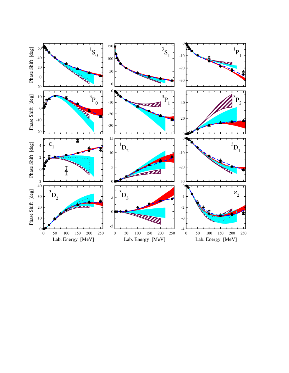
Figure 26: S–, P– and D–waves np phase shifts. The dashed, light shaded and dark shaded bands show the NLO, N²LO and N³LO [162] results, respectively. The dashed line is the N³LO result of Ref. [163]. The filled circles (open triangles) depict the results from the Nijmegen multi–energy PWA [108, 109] (Virginia Tech single–energy PWA [222]).

Low–energy observables should not depend on the cut–off(s) provided that all terms in the EFT expansion are included. In practice, however, calculations are performed at a finite order, so that some (small) residual dependence of observables on the cut–off(s) remains. One, in general, expects that this cut–off dependence gets weaker when higher order terms are included. While this is indeed the case for N³LO, the bands at NLO and N²LO are of comparable width. This does, however, not indicate any inconsistency as the following arguments show. The cut–off dependence of the scattering amplitude at both NLO and N²LO has to be compensated by inclusion of the counter terms (contact interactions) at order $\nu=4$ and higher. The contact interactions appear only at even orders $\nu=2n,\;n\geq 0$ in the low–momentum expansion while pion exchanges contribute, in general, at both even and odd orders. Since the same contact terms enter the expression for the effective potential at NLO and N²LO, a similar cut–off dependence for the observables at these orders should be expected. The results shown in Fig. 26 confirm these expectation.

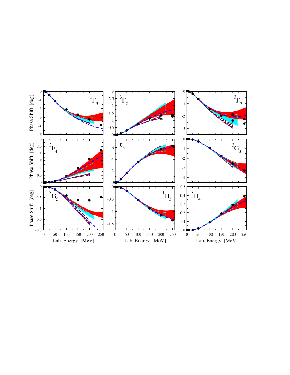
Figure 27: Selected peripheral np phase shifts. For notation see Fig. 26.

The uncertainty due to the cut–off variation in S–, P– and D–waves at N³LO agrees well with the estimation given above. For example, at $E_{\rm lab}=250$ MeV, the P–wave phase shifts at N³LO deviate from the data by an amount of up to $\sim 8^{\circ}$, which has to be compared with the typical size of the P–wave phase shifts at this energy of the order $\sim 25^{\circ}$. We further emphasize that all phase shifts at N³LO are visibly improved compared to N²LO (and NLO). The results at N³LO provide an accurate description of the data up to $E_{\rm lab}\sim 200$ MeV. It is comforting to see that the bands at N²LO and N³LO overlap (except in some channels at higher energies). As pointed out before, one cannot expect the same for the NLO bands, which underestimate the theoretical uncertainty at this order. Finally, we also show the N³LO results from Ref. [163] based on $\Lambda=500$ MeV. The two N³LO analyses agree with each other in all cases except some minor deviations in the partial waves ${}^{1}P_{1}$ and ${}^{3}D_{1}$ at intermediate and higher energies.

F– and selected higher partial waves, which are parameter–free at the considered orders, are shown in Fig. 27. In most channels, the predictions at N³LO are in agreement with the data. Contrary to the previously considered case of low partial waves, the bands do not get thinner at N³LO. This has to be expected due to the lack of the short–range contact terms in these channels. Such terms start to contribute to F–waves at N⁵LO ($\nu=6$) and to G–waves at N⁷LO ($\nu=8$). Consequently, a similar uncertainty due to the cut–off variation should be expected up to these high orders in the chiral expansion. The largest deviation from the data is observed for the ${}^{3}G_{5}$ partial wave. In this channel, the 1PE and the leading 2PE potentials are not sufficient to reproduce the PWA result at energies beyond $\sim 100$ MeV. The 2PE corrections at N²LO and N³LO improve the description of the data, but the effects are not big enough. This disagreement should, however, not be taken too seriously because of the exceptionally small size of the corresponding phase shift (more than 10 times smaller in magnitude compared to other G–waves). The N³LO predictions from Ref. [163] are also plotted in Fig. 27. They lie inside the N³LO bands from Ref. [162] in all cases with the exception of the ${}^{1}F_{3}$ and ${}^{3}G_{5}$ partial waves. The relatively large deviations in these two channels might be caused by the different values of $c_{i}$ (especially of the LEC $c_{4}$) adopted in [163].

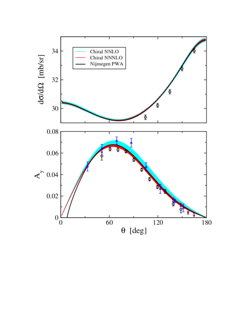
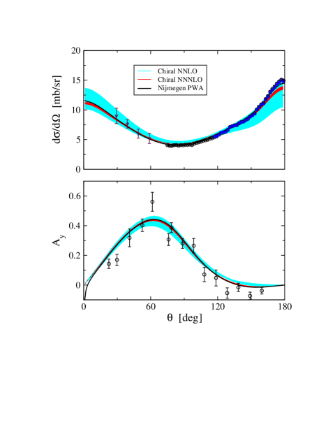
Figure 28: np differential cross section and vector analyzing power at $E_{\rm lab}=25$ MeV (left panel) and $E_{\rm lab}=96$ MeV (right panel). The Nijmegen PWA result is taken from [109]. The cut–offs $\Lambda$ and $\tilde{\Lambda}$ are varied as specified in Eq. (4.4). For data see [162].

Once the NN phase shifts are calculated, all two–nucleon scattering observables can be obtained in a straightforward way using e.g. the formulae collected in [180]. In Fig. 28 the np differential cross section and vector analyzing power at $E_{\rm lab}=$25 and 96 MeV at N²LO and N³LO from [162] are shown in comparison with the data and the Nijmegen PWA results. This calculation is based on np partial waves up to $j\leq 8$ and does not include the magnetic moment interaction. It is comforting to see that N²LO and N³LO results overlap and are in agreement with the Nijmegen PWA. The deviations in the analyzing power at forward direction are due to the neglected magnetic moment interaction. The small but visible deviations from the Nijmegen PWA for the differential cross section at forward and backward angles at N³LO are probably due to the neglect of partial waves with $j>8$.

We now regard the np S–wave scattering length and effective range parameters. The results at various orders in the chiral expansion are summarized in Table 5. All observables are improved when going from NLO to N²LO and from N²LO to N³LO. The N³LO result for the ${}^{1}S_{0}$ scattering length fills a small gap between the N²LO prediction and the value of the Nijmegen PWA. For the pp ${}^{1}S_{0}$ scattering length and effective range, the values $a_{pp}=-7.795\ldots-7.812$ fm and $r_{pp}=2.73\ldots 2.76$ fm were obtained at N³LO [162], which agree nicely with the data [251]: $a_{pp}^{\rm exp}=-7.8149\pm 0.0029$ fm and $r_{pp}^{\rm exp}=2.769\pm 0.014$ fm. The “standard value” for the nn scattering length, $a_{nn}^{\rm std}=-18.9$ fm, was used in [162] as an input parameter in order to pin down the LEC $\tilde{\beta}_{1S0}^{nn}$. The resulting prediction for the effective range, $r_{nn}=2.76\ldots 2.80$ fm, agrees with the experimental value, $r_{nn}^{\rm exp}=2.75\pm 0.11$ fm.

Finally, we would like to discuss various deuteron properties. The results at NLO, N²LO from [248] and N³LO from [162] are collected in Table 6 together with the experimental values. Notice that none of the deuteron properties were used in fits to determine the LECs. The predicted binding energy at N³LO is within 0.4% of the experimental value, which has to be compared with 1%–1.5% ($\sim$2%–2.5%) deviation at N²LO (NLO). The asymptotic S–wave normalization strength $A_{S}$ is also visibly improved at N³LO and deviates from the experimental (central) value by 0.3% as compared to $\sim$1.1% ($\sim$1.9%) at N²LO (NLO). The results for the asymptotic D/S–ratio at all orders are in agreement with the data within the experimental uncertainty. The N³LO result for $\eta_{\rm d}$ agrees well with the one of the Nijmegen PWA [252], $\eta_{\rm d}=0.0253(2)$. No improvement is observed for the quadrupole momentum $Q_{\rm d}$ at N³LO, which shows an even larger deviation from the data compared to N²LO (6%–8% versus 4%–5%). One should, however, keep in mind that the effects of the two–nucleon currents and relativistic corrections to this observable were not accounted for in the calculation of Ref. [162]. The situation with the deuteron rms-radius is similar to the one with the quadrupole moment: one observes a larger deviation from the data at N³LO as compared to the NLO and N²LO results. Notice however that the N³LO result for this quantity is still within 0.5% of the value from Ref. [253].

	NLO [248]	N2LO [248]	N3LO [162]	Nijmegen PWA
$a_{1S0}$ [fm]	$-23.447\ldots-23.522$	$-23.497\ldots-23.689$	$-23.585\ldots-23.736$	$-$23.739
$r_{1S0}$ [fm]	$2.60\ldots 2.62$	$2.62\ldots 2.67$	$2.64\ldots 2.68$	2.68
$a_{3S1}$ [fm]	$5.429\ldots 5.433$	$5.424\ldots 5.427$	$5.414\ldots 5.420$	$5.420$
$r_{3S1}$ [fm]	$1.710\ldots 1.722$	$1.727\ldots 1.735$	$1.743\ldots 1.746$	$1.753$

Table 5: np scattering length and effective range for the ${}^{1}S_{0}$ and ${}^{3}S_{1}$ partial waves at NLO, N²LO and N³LO compared to the Nijmegen PWA results [252, 254].

	NLO [248]	N2LO [248]	N3LO [162]	Exp
$E_{\rm d}$ [MeV]	$-2.171\ldots-2.186$	$-2.189\ldots-2.202$	$-2.216\ldots-2.223$	$-$2.224575(9)
$Q_{\rm d}$ [fm2]	$0.273\ldots 0.275$	$0.271\ldots 0.275$	$0.264\ldots 0.268$	0.2859(3)
$\eta_{\rm d}$	$0.0256\ldots 0.0257$	$0.0255\ldots 0.0256$	$0.0254\ldots 0.0255$	0.0256(4)
$\sqrt{\langle r^{2}\rangle^{\rm d}_{m}}$ [fm]	$1.973\ldots 1.974$	$1.970\ldots 1.972$	$1.973\ldots 1.985$	1.9753(11)
$A_{S}$ [fm-1/2]	$0.868\ldots 0.873$	$0.874\ldots 0.879$	$0.882\ldots 0.883$	0.8846(9)
$P_{\rm d}\;[\%]$	$3.46\ldots 4.29$	$3.53\ldots 4.93$	$2.73\ldots 3.63$	–

Table 6: Deuteron properties at NLO, N²LO and N³LO compared to the data. Here, $E_{\rm d}$ is the binding energy, $Q_{\rm d}$ the quadrupole moment, $\eta_{\rm d}$ the asymptotic $D/S$ ratio, $\sqrt{\langle r^{2}\rangle^{\rm d}_{m}}$ the root–mean–square matter radius, $A_{S}$ the strength of the asymptotic S–wave normalization and $P_{\rm d}$ the D-state probability. The data for $E_{\rm d}$ are from [255], for $Q_{\rm d}$ from [256, 257], for $\eta_{\rm d}$ from [258] and for $A_{S}$ from [257]. For the rms–radius we actually show the deuteron “point–nucleon” rms–radius from [253].

Last but not least, we would like to mention that the N³LO analysis of Ref. [163] based on the cut–off in the LS equation $\Lambda=500$ MeV was recently extended to $\Lambda=600$ MeV [259]. In most partial waves, very close results for both choices of $\Lambda$ with no visible differences for energies up to $300$ MeV were reported. This seems to be in contradiction with the expectations based on the arguments and estimations presented above: even if $\Lambda$ is chosen to be 500 MeV instead of 450 MeV as in Ref. [162], one can still expect only a very slow convergence of the low–momentum expansion at $E_{\rm lab}=300$ MeV, which corresponds to the CMS momentum $k\sim 375$ MeV. It would be interesting to see how sensitive the results of [163, 259] are to a particular form of the regulator in Eq. (4.5) with $n$ being chosen differently for different contributions to the potential.

4.1.4 Resonance saturation for NN contact interactions

In this section we would like to confront the LECs determined from chiral effective field theory with the highly successful phenomenological/meson exchange models of the nuclear force following the lines of Refs. [260, 248] and restricting ourselves to N²LO. Consider, for example, the Bonn–B [261] and Nijmegen 93 [262] potentials which are genuine one–boson–exchange (OBE) models. The long–range part of the interaction in these models is given by 1PE (including a pion–nucleon form factor) whereas shorter distance physics is expressed as a sum over heavier mesons exchange contributions. For nucleon momentum transfer below the masses of the exchanged mesons, one can interpret such exchange diagrams as a sum of local contact operators with an increasing number of derivatives (momentum insertions). The LECs accompanying the resulting contact interactions are given within each model in terms of the meson masses, meson–nucleon coupling constants and corresponding form–factors. We now wish to compare these LECs to the ones entering the chiral NN potential in order to see, whether they can be understood in terms of resonance saturation [260]. In order to allow for a meaningful comparison with the OBE models, one needs to properly account for the chiral 2PE potential, which is absent in the OBE models. To achieve that, the 2PE potential at NLO and N²LO is power expanded and the corresponding contributions to the LECs are identified, see [248] for more details on this procedure and for explicit analytical expressions. The second and third columns in Table 7 show the corresponding numerical results at NLO and N²LO for the SFR cut–off $\tilde{\Lambda}=600$ MeV.

LEC	2PE (NLO)	2PE (N2LO)	$C_{i}$ (NLO)	$C_{i}$ (N2LO)	Bonn B	Nijm-93
$\tilde{C}_{1S0}$	$-0.004{{+0.000}\atop{-0.001}}$	$-0.004{{+0.000}\atop{-0.001}}$	$-0.117{{+2.271}\atop{-0.042}}$	$-0.158{{+0.178}\atop{-0.004}}$	$-0.117$	$-0.061$
${C}_{1S0}$	$-0.570{{+0.036}\atop{-0.022}}$	$-0.443{{+0.078}\atop{-0.057}}$	$1.294{{+2.873}\atop{-0.322}}$	$1.213{{+0.408}\atop{-0.084}}$	$1.276$	$1.426$
$\tilde{C}_{3S1}$	$0.013{{+0.001}\atop{-0.000}}$	$-0.004{{+0.000}\atop{-0.001}}$	$-0.135{{+0.025}\atop{-0.021}}$	$-0.137{{+0.017}\atop{-0.027}}$	$-0.101$	$-0.014$
${C}_{3S1}$	$0.638{{+0.025}\atop{-0.044}}$	$-0.443{{+0.078}\atop{-0.057}}$	$0.231{{+0.112}\atop{-0.007}}$	$0.523{{+0.197}\atop{-0.039}}$	$0.660$	$0.940$
${C}_{\epsilon 1}$	$-0.190{{+0.012}\atop{-0.006}}$	$0.205{{+0.024}\atop{-0.035}}$	$-0.325{{+0.000}\atop{-0.036}}$	$-0.395{{+0.007}\atop{-0.072}}$	$-0.410$	$-0.343$
${C}_{1P1}$	$-0.067{{+0.007}\atop{-0.005}}$	$-0.090{{+0.013}\atop{-0.009}}$	$0.146{{+0.005}\atop{-0.010}}$	$0.126{{+0.023}\atop{-0.017}}$	$0.454$	$0.119$
${C}_{3P0}$	$-0.425{{+0.025}\atop{-0.014}}$	$0.006{{+0.003}\atop{-0.003}}$	$0.923{{+0.142}\atop{-0.103}}$	$0.920{{+1.063}\atop{-0.109}}$	$0.921$	$0.802$
${C}_{3P1}$	$0.246{{+0.009}\atop{-0.016}}$	$0.247{{+0.032}\atop{-0.044}}$	$-0.260{{+0.003}\atop{-0.005}}$	$-0.108{{+2.364}\atop{-0.176}}$	$-0.075$	$-0.197$
${C}_{3P2}$	$-0.022{{+0.000}\atop{-0.000}}$	$0.151{{+0.020}\atop{-0.028}}$	$-0.262{{+0.032}\atop{-0.073}}$	$-0.421{{+0.074}\atop{-0.052}}$	$-0.396$	$-0.467$

Table 7: The LECs $C_{i}$ at NLO and N²LO compared with the results from the Bonn B and Nijmegen 93 OBE potential models. Also shown are contributions from chiral 2PE as explained in text. The $\tilde{C}_{i}$ are in 10⁴ GeV^-2 and the $C_{i}$ in 10⁴ GeV^-4.

The indicated uncertainty refers to the cut–off variation $\tilde{\Lambda}=500\ldots 700$ MeV. The fourth and fifth columns contain the values of the LECs $C_{i}$ at NLO and N²LO, where the just discussed contributions from 2PE have already been added. The numbers are presented for the cut–off combination $\{\Lambda,\;\tilde{\Lambda}\}=\{550,\;600\}$ with the uncertainties referring to the variations: $\tilde{\Lambda}=500\ldots 700$ MeV and $\Lambda=450\ldots 600$ MeV ($\Lambda=450\ldots 650$ MeV) at NLO (N²LO). Notice that in certain cases, $C_{i}$’s show a rather strong cut–off dependence. This happens if the cut–off $\Lambda$ becomes too large (i.e. close to the critical value, at which spurious bound states arise) and one leaves the plateau–region for the corresponding LEC $C_{i}(\Lambda)$. This situation is exemplified in Fig. 25. Clearly, it only makes sense to discuss resonance saturation of the $C_{i}$’s in the plateau–region of the first branch, where they only change modestly and where the effective potential is, at least, not strongly non–phase–equivalent to the OBE models. The last two columns in Table 7 show the LECs as predicted by resonance saturation based upon the Nijmegen 93 and Bonn B potential models. One observes a remarkable agreement between the LEC values obtained from fit to NN phase shifts in the EFT approach and the ones resulting from the OBE models. For a related study based on a toy–model, the reader is referred to Ref. [263].

4.1.5 Quark mass dependence of the nuclear force

Since the absolute values of the running up and down quark masses at the scale 1 GeV, $m_{u}\simeq 5$ MeV, $m_{d}\simeq 9$ MeV, are rather small [184], one expects that hadronic properties at low energies do not change strongly in the chiral limit (CL) of $M_{\pi}\rightarrow 0$. This feature is crucial for the chiral expansion to make sense and is certainly true for the pion and pion–nucleon systems, where the interaction becomes arbitrarily weak in the CL and for vanishing external momenta. The situation in the few–nucleon sector is significantly more complicated due to the nonperturbative nature of the problem and also due to the fact that the interaction between nucleons does not become weak in the chiral limit. The $M_{\pi}$–dependence of the nuclear force can naturally be studied in the chiral EFT framework. It is not only of academic interest, but also relevant for interpolating the results from lattice gauge theory, see also [114]. For example, the S–wave scattering lengths have been calculated on the lattice using the quenched approximation [264]. Another interesting application is related to imposing bounds on the time–dependence of fundamental couplings from the two–nucleon sector, as discussed in [265].

The first, pioneering study of the NN system for vanishing quark masses was performed by Bulgac et al. [266] based upon the explicit $M_{\pi}$–dependence of the 1PE potential. More advanced studies and extensive discussion on this topic can be found in Refs. [114, 267, 134, 268, 269]. Here, we follow the lines of Ref. [134], where the $M_{\pi}$–dependence of the nuclear force on the pion mass was analyzed at NLO based on the DR potential in the limit of exact isospin symmetry. We remind the reader that the potential at this order is given by the 1PE and 2PE contributions and contact interactions with up to two derivatives or one $M_{\pi}^{2}$–insertion as detailed in section 3.2.2. In addition, one has to include the corrections to 1PE and the leading contact terms at the one–loop level, which lead to renormalization of the corresponding LECs and therefore induce implicit quark mass dependence. These corrections are discussed in detail in [134]. For the 1PE potential

$$V_{1\pi}=-\left(\frac{g_{\pi N}}{2m_{N}}\right)^{2}\,\mbox{\boldmath$\tau$}_{1}\cdot\mbox{\boldmath$\tau$}_{2}\,\frac{(\vec{\sigma}_{1}\cdot\vec{q}\,)(\vec{\sigma}_{2}\cdot\vec{q}\,)}{\vec{q}\,^{2}+M_{\pi}^{2}}\,,$$ (4.8)

with $g_{\pi N}$ being the pion–nucleon coupling constant, one has to account not only for explicit $M_{\pi}$–dependence in the denominator, but also for implicit dependence of the ratio $g_{\pi N}/m_{N}$ on the pion mass. For an arbitrary value $\tilde{M}_{\pi}$ of the pion mass one obtains [134]:

$$\frac{g_{\pi N}}{m_{N}}=\frac{g_{A}}{F_{\pi}}\Bigg{(}1-\frac{g_{A}^{2}\tilde{M}_{\pi}^{2}}{4\pi^{2}F_{\pi}^{2}}\ln\frac{\tilde{M}_{\pi}}{M_{\pi}}-\frac{2\tilde{M}_{\pi}^{2}}{g_{A}}\bar{d}_{18}+\left(\frac{g_{A}^{2}}{16\pi^{2}F_{\pi}^{2}}-\frac{4}{g_{A}}\bar{d}_{16}+\frac{1}{16\pi^{2}F_{\pi}^{2}}\bar{l}_{4}\right)(M_{\pi}^{2}-\tilde{M}_{\pi}^{2})\Bigg{)}\,,$$ (4.9)

where $g_{A}=1.26$, $F_{\pi}=92.4$ MeV and $M_{\pi}=138$ MeV denote the physical values of the nucleon axial vector coupling, pion decay constant and pion mass, respectively. Further, $\bar{l}_{4}$, $\bar{d}_{18}$ and $\bar{d}_{16}$ are LECs related to pion and pion–nucleon interactions. Following Ref. [134], we use $\bar{l}_{4}=4.3$ [6], $\bar{d}_{16}=-1.23{{+0.32}\atop{-0.53}}$ GeV^-2 [270, 271] and $\bar{d}_{18}=-0.97$ GeV^-2. The constant $\bar{d}_{18}$ is determined from the observed value of the Golberger–Treiman discrepancy with $g_{\pi N}=13.2$ [272]. Notice further that for the LEC $\bar{d}_{16}$, we use an average of three values given in [271], which result from different fits. The shown uncertainty is defined in the way to cover the whole range of values from [271].

The remaining $\tilde{M}_{\pi}$–dependence of the nuclear force at NLO is given by 2PE, see Eq. (3.2.2), and by the short–range terms of the form

$$V^{\tilde{M}_{\pi}}_{\rm cont}=\tilde{M}_{\pi}^{2}\,\Bigg{(}\bar{D}_{S}+\bar{D}_{T}(\vec{\sigma}_{1}\cdot\vec{\sigma}_{2})-\left(\beta_{S}+\beta_{T}(\vec{\sigma}_{1}\cdot\vec{\sigma}_{2})\right)\ln\frac{\tilde{M}_{\pi}}{M_{\pi}}\Bigg{)}\,,$$ (4.10)

where the constants $\beta_{S,T}$ are given in terms of $g_{A}$, $F_{\pi}$ and $C_{T}$ [273]. All other contact terms do not depend on the pion mass and the corresponding LECs were adopted in [134] from the analysis of [139], performed for the physical value $\tilde{M}_{\pi}=M_{\pi}$. The essential difficulty in extrapolating the nuclear forces in the pion mass is due to the fact that the LECs $\bar{D}_{S}$, $\bar{D}_{T}$ cannot be fixed from the NN data. In order to proceed further, natural values for these LECs were assumed in [134]

$$\bar{D}_{S,T}=\frac{\alpha_{S,T}}{F_{\pi}^{2}\Lambda_{\rm LEC}^{2}}\,,\quad\mbox{where}\quad-3.0<\alpha_{S,T}<3.0\,,$$ (4.11)

based on $\Lambda_{\rm LEC}\simeq 1$ GeV. This estimation is consistent with the size of other contact terms with the corresponding dimensionless coefficients $\alpha_{i}$ lying in the range $-2.1\ldots 3.2$ [260].

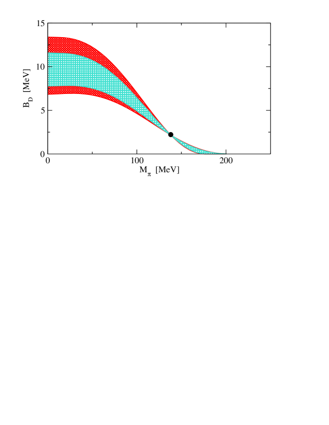
Figure 29: Deuteron BE versus the pion mass. The shaded areas show allowed values. The light (dark) shaded band depicts the uncertainty due to the unknown LECs $\bar{D}_{S,T}$ ($\bar{d}_{16}$). The heavy dot shows the BE for the physical case $\tilde{M}_{\pi}=M_{\pi}$.

The resulting deuteron binding energy (BE) as a function of the pion mass is shown in Fig. 29. The deuteron becomes unbound for $\tilde{M}_{\pi}\gtrsim 170$ MeV and is found to be stronger bound in the chiral limit with the BE $B_{\rm D}^{\rm CL}=9.6\pm 1.9{{+1.8}\atop{-1.0}}$ MeV [134]. Here, the first indicated error refers to the uncertainty in the value of $\bar{D}_{{}^{3}S_{1}}$ and $\bar{d}_{16}$ being set to the average value $\bar{d}_{16}=-1.23$ GeV^-2 while the second indicated error shows the additional uncertainty due to the uncertainty in the determination of $\bar{d}_{16}$ as described above. Other deuteron properties in the chiral limit are discussed in [273]. The resulting values for the two S–wave scattering lengths in the chiral limit are smaller in magnitude and more natural: $a_{\rm CL}(^{1}S_{0})=-4.1\pm 1.6{{+0.0}\atop{-0.4}}\,$fm and $a_{\rm CL}(^{3}S_{1})=1.5\pm 0.4{{+0.2}\atop\\ {-0.3}}\,$fm. As pointed out in [134], one needs lattice data for pion masses below 200 MeV to be able to perform a stable extrapolation to its physical value. Last but not least, we emphasize that the analysis of [268], see also [274] for a related work, assumes a significantly larger uncertainty in the values of the LECs $\bar{D}_{S,T}$ and $\bar{d}_{16}$, which is the main reason of different results for the ${}^{3}S_{1}$ channel reported in that work. For an extended discussion on this issue, the reader is referred to [269]. We also emphasize that the work of [275] seems to indicate the importance of including $\Delta$’s as explicit degrees of freedom in order to properly describe the quark mass dependence of the nucleon axial–vector coupling constant. Notice further that effects due to radiative pions might become important close to the CL. Finally, the possibility of an infrared renormalization group limit cycle in the 3N sector is discused in [276].

4.2 The three– and four–nucleon systems up to N²LO

We now turn to systems with three and four nucleons, which serve as an excellent testing ground for chiral forces and allow for a highly nontrivial check of the consistency of this approach since most of the unknown LECs are already determined in the NN system.

The first quantitative application of chiral forces to $Nd$ scattering in the 3N and 4N sectors was performed in [277] at NLO. To that aim, the Faddeev–Yakubovsky equations were solved rigorously for the 3N and 4N systems and the corresponding binding energies as well as various 3N scattering observables were computed. Since no 3NF appears at this order in the chiral expansion, the study of [277] was entirely based on the 2NF yielding parameter–free results for the 3N and 4N systems. This work used the DR version of the chiral 2N potential with the LS cut–off varied in the range $\Lambda=540\ldots 600$ MeV and demonstrated a good description of the $nd$ elastic scattering data at $E_{\rm lab}=3$ MeV and $E_{\rm lab}=10$ MeV as well as of some break–up observables at $E_{\rm lab}=13$ MeV. The predictions for the triton and $\alpha$–particle BE were found to be in a similar range as the ones based on phenomenological NN potentials.

The NLO analysis of [277] was extended to incomplete N²LO in [214] where the 2N potential at N²LO was used without taking into account the corresponding 3NF. The first complete analysis of $nd$ scattering at this order including the 3NF was presented in Ref. [194]. Both calculations of [214] and [194] used the DR 2N potential with the numerically reduced values of $c_{3,4}$ in order to avoid the appearance of spurious bound states, see section 4.1.3 for more details. In addition, certain $nd$ scattering observables were studied in [278] using the 2N potential from [247] with no 3NF included.

Recently, the 3N and 4N systems were reanalyzed at NLO and N²LO within the SFR framework [279]. We remind the reader that the SFR 2N potential at N²LO is based on the LECs $c_{i}$ which are consistent with $\pi N$ scattering. This is an important advantage compared to the previous study in Ref. [194]. Notice that these LECs also determine the strength of the 2PE 3NF. In addition, larger cut–off variation adopted in [162] is expected to provide a more realistic estimation of the theoretical uncertainty. In the following sections we will present some results for 3N and 4N observables based on the SFR 2NF. Further details and more results will be published elsewhere [279]. In selected cases, we will compare the results based on the SFR and DR 2N potentials from Refs. [162] and [214]. Further applications of chiral nuclear forces to 3N scattering can be found in Refs. [280, 281, 282, 283, 284].

4.2.1 The formalism

To describe the properties of the 3N and 4N systems, a corresponding Schrödinger equation needs to be solved. As described in section 4.1.3, we use a specific form for the regularization of the potential, which allows us to determined the LECs of the NN force partial wave by partial wave. This, however, implies that the interactions are strongly non–local. Therefore, a formulation in momentum space is most natural.

In the past, the techniques were developed for solving reliably the Schrödinger equation in momentum space using Faddeev– or Yakubovsky equations [285, 286]. For the 3N bound state problem, the Faddeev equations have the form [287]

$$\psi=G_{0}\,t\,P\,\psi+(1+G_{0}\,t)\,G_{0}\,V_{123}^{(1)}\,(1+P)\,\psi\,.$$ (4.12)

Here $V_{123}^{(i)}$ is that part of the 3N force which singles out the particle $i$ and which is symmetrical under the exchange of the other two particles. The complete 3NF is decomposed as

$$V_{123}=V_{123}^{(1)}+V_{123}^{(2)}+V_{123}^{(3)}\,.$$ (4.13)

Further, $\psi$ denotes the corresponding Faddeev component, $t$ is the two–body $t$–operator, $G_{0}=1/(E-H_{0})$ is the free propagator of three nucleons and $P$ is a sum of a cyclical and anticyclical permutation of the three particles. In case of $nd$ scattering we follow the formulation described in Refs. [285, 288] and first calculate a quantity $T$ related to the 3N break–up process via the Faddeev–like equation:

$$T=t\,P\,\phi+(1+t\,G_{0})\,V_{123}^{(1)}\,(1+P)\,\phi+t\,P\,G_{0}\,T+(1+t\,G_{0})\,V_{123}^{(1)}\,(1+P)\,G_{0}\,T\,,$$ (4.14)

where the initial state $\phi$ is composed of a deuteron and a momentum eigenstate of the projectile nucleon. The elastic $nd$ scattering operator is then obtained as

$$U=P\,G_{0}^{-1}+P\,T+V_{123}^{(1)}\,(1+P)\,(1+G_{0}\,T)\,,$$ (4.15)

and the break–up operator via

$$U_{0}=(1+P)\,T\,.$$ (4.16)

These equations are accurately solved in momentum space using a partial wave decomposition, see [289, 290, 291] for details. The partial wave decomposition of the chiral 3NF is given in the appendix of Ref. [194].

Similarly, we use Yakubovsky equations (YE) to solve the 4N bound state problem. We rewrite the Schrödinger equation into two YEs and thus decompose the wave function $\Psi$ into two independent Yakubovsky components (YCs): $\psi_{1}$ and $\psi_{2}$ [286, 292, 293]. The wave function then reads

$$\Psi=(1-(1+P)\ P_{34})(1+P)\psi_{1}+(1+P)\ (1+\tilde{P})\psi_{2}$$ (4.17)

and is again expressed with the help of the permutations $P$ and $\tilde{P}=P_{13}P_{24}$ where $P_{ij}$ denotes transpositions of particles $i$ and $j$. In the case of a bound state it is, in principle, possible to solve directly the Schrödinger equation. The usage of two YCs is, however, advantageous since it naturally introduces two kinds of Jacobi coordinates which accelerates the convergence of the partial wave decomposition [293]. The YEs reduce to two coupled integral equations

$$\psi_{1} = G_{0}\ t\ P\left[(1-P_{34})\psi_{1}+\psi_{2}\right]+(\ 1+G_{0}\ t\ )G_{0}V_{123}^{(3)}\Psi$$ (4.18)

$$\psi_{2} = G_{0}\ t\ \tilde{P}\ \left[(1-P_{34})\ \psi_{1}+\psi_{2}\right]\,,$$ (4.19)

which can be solved by similar techniques as the 3N problem. The high dimensionality (up to $10^{8}\times 10^{8}$) of the discretized YEs, however, requires massively parallel computers.

Because these techniques are formulated in momentum space, the application of long–range interactions, like the $pp$ Coulomb force, is a major difficulty. For the scattering problem, we therefore neglect the Coulomb interaction completely. At higher energies (above 50 MeV nucleon lab energy), it is expected to contribute mainly in forward direction. Here, the comparison of our results to the data should be less affected by the missing electromagnetic forces. For lower energies, we will compare our results to modified data, which have been corrected for the electromagnetic interactions using calculations of Alejandro Kievsky [294] based on the AV18 [295] interactions with and without the electromagnetic forces. For the bound states, we include the $pp$ Coulomb interactions in the $t$–matrices. Since the bound nucleons are confined to a small space region, we can put the Coulomb interaction to zero outside a radius of $10-20$ fm, effectively making it short–ranged. Then the Fourier transformation of this interaction is nonsingular. The results are cut–off independent and numerically stable.

4.2.2 Elastic Nd scattering

Consider now elastic $nd$ scattering. At N²LO, one has to take into account the 3NF which is discussed in section 3.3.1. Similarly to the 2N potential, the chiral 3NF behaves unphysically at large momenta and leads to ultraviolet divergences in the Faddeev–Yakubovsky equations. In [279], regularization was performed in the way analogous to the one adopted in the analysis of the 2N system:

$$V^{\rm 3NF}(\vec{p},\vec{q};\,\vec{p}\,^{\prime},\vec{q}\,^{\prime})\rightarrow f^{\Lambda}(\vec{p},\vec{q})\,V^{\rm 3NF}(\vec{p},\vec{q};\,\vec{p}\,^{\prime},\vec{q}\,^{\prime})\,f^{\Lambda}(\vec{p}\,^{\prime},\vec{q}\,^{\prime})\,,\quad\quad f^{\Lambda}(\vec{p},\vec{q}\,)=e^{-\left(\frac{4p^{2}+3q^{2}}{4\Lambda^{2}}\right)^{3}}\,,$$ (4.20)

where $\vec{p}$ and $\vec{q}$ ($\vec{p}\,^{\prime}$ and $\vec{q}\,^{\prime}$) are Jacobi momenta of the two–body subsystem and spectator nucleon before (after) the interaction. The regulator function $f^{\Lambda}(\vec{p},\vec{q}\,)$ is chosen so that for $\vec{q}=0$ it coincides with the function $f^{\Lambda}(\vec{p}\,)$ in Eq. (4.3). The results presented here and in what follows are based on the variation of the LS cut–off $\Lambda$ in the range $\Lambda=400\ldots 550$ at NLO and $\Lambda=450\ldots 600$ at N²LO. The SFR cut–off $\tilde{\Lambda}$ is varied in both cases in the range $\tilde{\Lambda}=500\ldots 700$ MeV. Specifically, the following cut–off combinations $\{\Lambda,\;\tilde{\Lambda}\}$ were used at NLO and N²LO:

$$\mbox{NLO}: \{\Lambda,\;\tilde{\Lambda}\}=\{400,\;500\},\;\{550,\;500\},\;\{550,\;600\},\;\{400,\;700\},\;\{550,\;700\}\,,$$

$$\mbox{N${}^{2}$LO}: \{\Lambda,\;\tilde{\Lambda}\}=\{450,\;500\},\;\{600,\;500\},\;\{550,\;600\},\;\{450,\;700\},\;\{600,\;700\}\,.$$ (4.21)

As explained in section 3.3.1, the chiral 3NF at N²LO is given by the two–pion exchange, one–pion exchange with the pion emitted (or absorbed) by 2N contact interactions and 3N contact interactions. While the 2PE contribution given in Eq. (3.72) does not introduce any new parameters, the two other terms depend on two new LECs, $D$ and $E$, cf. Eq. (3.73), which are not determined in the 2N system and thus need to be fixed e.g. from the 3N data. As demonstrated in Ref. [194], they can be determined using the ³H BE and the $nd$ doublet scattering length ${}^{2}a_{nd}$, which are bona fide low–energy observables. In the present analysis, we use the coherent $nd$ scattering length $b_{nd}$ instead of the ${}^{2}a_{nd}$. This quantity is defined in terms of the doublet and quartet $nd$ scattering lengths ${}^{2}a_{nd}$ and ${}^{4}a_{nd}$ and the neutron/deuteron masses as

$$b_{nd}=\frac{m_{n}+m_{d}}{m_{d}}\left[\frac{1}{3}\,^{2}a_{nd}+\frac{2}{3}\,^{4}a_{nd}\right]\,,$$ (4.22)

where ${}^{4}a_{nd}$ is the $nd$ quartet scattering length and $m_{n}$ ($m_{d}$) refers to the neutron (deuteron) mass. The coherent $nd$ scattering length is much better known experimentally than ${}^{2}a_{nd}$, which allows to reduce the uncertainty in the determination of the LECs $D$ and $E$. The resulting LECs are found to be of natural size, i.e. the constants $c_{D}$ and $c_{E}$ defined as

$$D=\frac{c_{D}}{F_{\pi}^{2}\Lambda_{\rm LEC}}\,,\quad\quad E=\frac{c_{E}}{F_{\pi}^{4}\Lambda_{\rm LEC}}\,,$$ (4.23)

are of order one. The only exception is given by the cut–off combination $\{600,\;500\}$, for which the magnitude of $c_{D}$ is rather large ($c_{D}=-10.0$ for $\Lambda_{\rm LEC}=700$ MeV). Notice further that the values for both LECs depend strongly on the cut–offs and differ significantly from the ones found in an earlier study [194]. Finally, we would like to emphasize that the ³H BE and the central experimental value of $b_{nd}$ could be reproduced simultaneously only for $\{\Lambda_{i},\;\tilde{\Lambda}_{i}\}$ in Eq. (4.2.2) with $i=1,3,4$. For two other cut–off combinations, it was not possible to find a solution for $c_{D}$ and $c_{E}$, which would describe both observables at the same time. In these cases, the scattering length $b_{nd}$ (the triton BE) was required to be reproduced exactly (as good as possible). We will discuss the resulting ³H BE in section 4.2.4. More details on fixing the values of $c_{D}$ and $c_{E}$ will be given in [279].

	$\pi/$ EFT, N2LO	NLO	N2LO	Exp
${}^{2}a_{nd}$	$-$	$0.61\ldots 1.19$	$0.61\ldots 0.63$	$0.65\pm 0.04$ [296]
${}^{4}a_{nd}$	$6.33\pm 0.05$	$6.360\ldots 6.366$	$6.353\ldots 6.362$	$6.35\pm 0.02$ [296]
$b_{nd}$	$-$	$6.656\ldots 6.959$	$6.669^{\star}$	$6.669\pm 0.003$ [297]

Table 8: $nd$ scattering lengths (in fm) in EFT in comparison with the data. For NLO and N²LO in the EFT with explicit pions, the cut-offs $\Lambda$ and $\tilde{\Lambda}$ are varied in the range given in Eq. (4.2.2). The value of $b_{nd}$ used as input is marked by the star.

In Table 8 we summarize the EFT results for various $nd$ scattering lengths in comparison with the experimental numbers. In the case of pionless EFT, the value shown in this table is taken from Ref. [95], where more discussion on this approach and further references to earlier determinations of ${}^{4}a_{nd}$ can be found.

With the LECs $c_{D}$ and $c_{E}$ being determined as described above, we are now in the position to predict various $nd$ elastic scattering observables. In Fig. 30 we show the results for the differential cross section (in the left column) and vector analyzing power (in the right column) at $3$, $10$ and $65$ MeV. One observes a good agreement with the data at two lowest energies at both NLO and N²LO. This also holds true for tensor analyzing powers shown in Fig. 31 for $E_{\rm lab}=10$ MeV. The only exceptions are given by the minima of $T_{20}$ and $T_{21}$ at N²LO, where some deviations from the data are visible. We remind the reader that the data at energies 3 and 10 MeV have been corrected to account for the missing Coulomb force [294]. The uncertainty due to the cut–off variation in the differential cross section is significantly reduced at N²LO compared to NLO at all energies considered. At 65 MeV, the results at NLO show large deviations from the data in the minimum of the cross section as well as for $A_{y}$. Similarly to the 2N system, the bands at NLO seem to underestimate the true theoretical uncertainty at this order, see section 4.1.3 for more discussion. The N²LO results at 65 MeV are in agreement with the data for both observables.

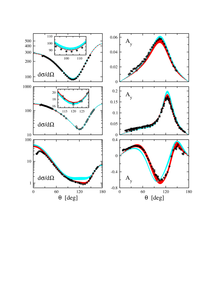
Figure 30: Differential cross section (in mb/sr) and vector analyzing power for elastic $nd$ scattering at 3 MeV (upper panel) 10 MeV (middle panel) and 65 MeV (bottom panel) at NLO (light–shaded bands) and N²LO (dark–shaded bands) in the SFR framework. The bands correspond to the cut–off variation as specified in Eq. (4.2.2). For data see [194].

Notice that the deviation from the data for $d\sigma/d\Omega$ in forward directions is due to the Coulomb force which is missing in the calculations. At this energy, the uncertainty at N²LO appears to be rather large. For the tensor analyzing powers at the same energy, the situation is similar: while the NLO results deviate significantly from the data, the N²LO predictions are in agreement with the data but the uncertainty due to the cut–off variation is large. A more detailed discussion will be given in [279].

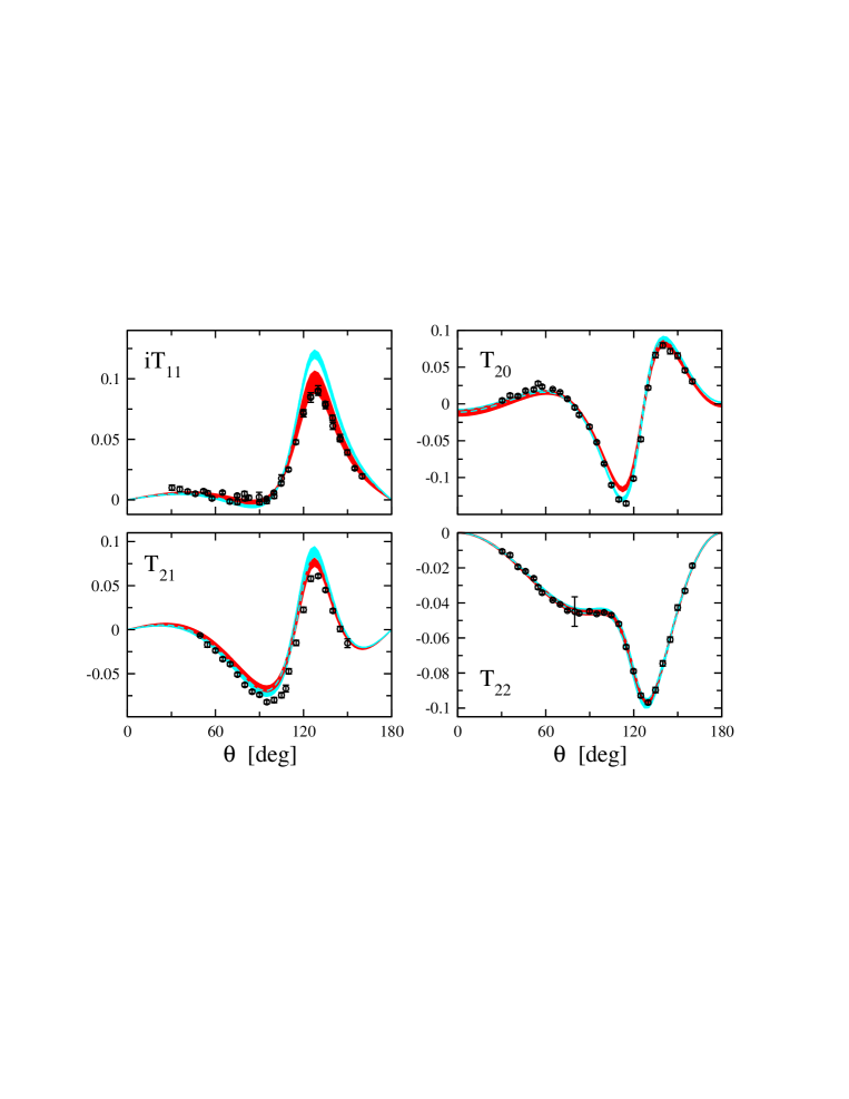
Figure 31: Tensor analyzing powers for elastic $nd$ scattering at 10 MeV at NLO (light–shaded bands) and N²LO (dark–shaded bands). The bands correspond to the cut–off variation as specified in Eq. (4.2.2). For data see [194].

Let us now discuss the nucleon vector analyzing power $A_{y}$, which is the most problematic observable in $nd$ elastic scattering at low energy. This particular observable is underpredicted in the maximum by an amount of $\sim 25\ldots 30$% by modern high–precision nuclear potentials, which is known in the literature as $A_{y}$ puzzle [298, 299]. Augmenting the NN potentials with 3NF models such as the TM99’ 3NF [300] or the Urbana-IX 3NF [301], which are frequently used in modern few–body calculations, does not substantially improve the description of this observable. The only exception is given by the phenomenological spin–orbit 3NF introduced by Kievsky [302], which allows to describe the data. Similar discrepancies (but less pronounced compared to $A_{y}$) are also observed for the tensor analyzing power $iT_{11}$. As demonstrated in Fig. 30, The NLO result for $A_{y}$ is in agreement with the data at 3 MeV and even slightly overpredicts the data at 10 MeV. Very similar results based on the DR NN potential at NLO were obtained in [277, 214]. While this looks encouraging, one cannot conclude that the $A_{y}$–puzzle has been solved. This observable is well known to be very sensitive to the spin–orbit 2NF and, therefore, to the triplet P–waves, see e.g. [285, 278], which need to be reproduced accurately in order to have conclusive results. It is instructive to look at the spin–orbit phase shift combination $\Delta_{LS}$ defined as [278]:

$$\Delta_{LS}=\frac{1}{12}\left(\ 2\delta_{{}^{3}P_{0}}-3\delta_{{}^{3}P_{1}}+5\delta_{{}^{3}P_{2}}\right)\,.$$ (4.24)

In Table 9, we show the results for this quantity at NLO and N²LO compared to the ones from Nijmegen PWA. Clearly, the spin–orbit force at NLO is enhanced compared to Nijmegen PWA, which also explains the enhancement for $nd$ $A_{y}$ at this order. Notice that the overestimation of $\Delta_{LS}$ at NLO (and, to a less extend, also at N²LO) is largely due to the failure to properly describe the ${}^{3}P_{2}$ partial wave, cf. Fig. 26. We emphasize, however, that the quantity $\Delta_{LS}$ is more accurately reproduced at N²LO, where the calculated $nd$ $A_{y}$ is in a reasonable agreement with the data (although the uncertainty due to the cut–off variation appears to be quite sizable). A more detailed discussion including the role of the 3NF will be given in [279], see also [303] for a related earlier work.

Finally, we emphasize that at low energy the results for $nd$ elastic scattering observables at NLO and N²LO in both SFR and DR [214] frameworks are very similar. The strongest differences are observed for $A_{y}$ and $iT_{11}$, where the N²LO correction is larger in the DR approach. Very different values of $c_{3,4}$ adopted in these analyses, which determine the strength of the 2PE 3NF, have only a little impact on the considered $nd$ elastic scattering observables. At higher energies such as 65 MeV, the differences between the two sets of calculations, however, become quite significant. For further results in $nd$ elastic scattering based on the NN potential of Ref. [247] the reader is referred to [278].

$E_{\rm lab}$ (MeV)	NLO	N2LO	Nijmegen PWA
$10$	$0.201\ldots 0.210$	$0.183\ldots 0.199$	$0.202$
$20$	$0.694\ldots 0.721$	$0.622\ldots 0.673$	$0.641$
$30$	$1.46\ldots 1.51$	$1.28\ldots 1.39$	$1.25$
$40$	$2.43\ldots 2.54$	$2.10\ldots 2.28$	$1.97$
$50$	$3.57\ldots 3.76$	$2.97\ldots 3.30$	$2.73$

Table 9: Spin–orbit combination $\Delta_{LS}$ for $np$ phase shifts (in degrees) at various energies at NLO and N²LO in comparison with the result of Nijmegen PWA [109]. The cut-offs are chosen as in Eq. (4.2.2).

4.2.3 Nd break–up

Let us now switch to break–up observables. In the following, we will show some results at two energies, 13 and 65 MeV, where a lot of $pd$ data exist. Since we do not have reliable Coulomb corrections in the case of break–up, we show the non–corrected $pd$ data in comparison to our $nd$ calculations.

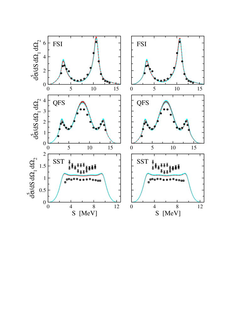
Figure 32: $nd$ break–up cross section in [mb MeV^-1 sr^-2] along the kinematical locus $S$ at 13 MeV in comparison to predictions at NLO (light shaded band) and N²LO (dark shaded band) in the chiral EFT. In the left (right) panel, the results based on the SFR (DR) scheme are shown. In the upper row a final state interaction configuration is depicted, in the middle one a quasi–free scattering configuration (both in comparison to $pd$ data) and in the lower one a space star configuration (upper data $nd$, lower data $pd$). The precise kinematical description and references to data can be found in Ref. [285].

In Fig. 32 we present the results for a few often investigated configurations, the space-star (SST), a final state interaction (FSI) peak configuration and a quasi–free scattering (QFS) configuration, respectively. For a general discussion on various break–up observables and configurations the reader is referred to [285]. As demonstrated in Fig. 32, the results at 13 MeV are very robust and essentially the same at NLO and N²LO in both the SFR and DR approaches. The description of the configuration dominated by FSI peaks is rather accurate (for a more elaborated procedure the angular openings of the detectors have to be taken into account, see [285]). The present theory for the break–up configuration including a QFS geometry fails in the central maximum. This might be due to missing Coulomb force effects. The third configuration, the so called space–star, is one of the long standing puzzles of 3N scattering, see e.g. [304]. Similar to the phenomenological interactions, we even fail to describe the $nd$ data. The strong deviation between the $nd$ and $pd$ data indicates the importance of the Coulomb effects for this particular configuration. It is still an open question whether the $pd$ data can be reproduced by the theory if Coulomb force is taken into account.

     

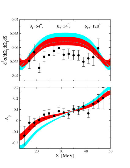
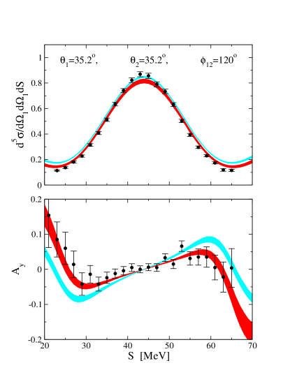
Figure 33: $nd$ break–up cross section in [mb MeV^-1 sr^-2] and nucleon analyzing power along the kinematical locus $S$ (in MeV) at 65 MeV in comparison to predictions at NLO (light shaded band) and N²LO (dark shaded band) in chiral effective field theory. The cut-offs $\Lambda$ and $\tilde{\Lambda}$ are chosen as in Eq. (4.2.2). The left and right panels show the symmetric space star and symmetric forward star configurations, respectively. $pd$ data are from [305].

At 65 MeV we show in Fig. 33 the results for the cross section and nucleon vector analyzing power for two selected configurations. These and other configurations were studied in the context of phenomenological nuclear forces [306] as well in the chiral EFT based on the DR potential [194]. The situation at 65 MeV seems, in general, to be promising. In most cases, a clear improvement in the description of the data is observed when going from NLO to N²LO. We stress, however, that the uncertainty due to the cut–off variation is rather large at this energy. More results for break–up observables at this energy will be given in [279], see also [283].

In addition, we would like to mention some further recent studies, where the results based on chiral EFT were shown. Differential cross section of the ²H$(p,\,pp)n$ reaction at the proton energy 16 MeV in three kinematical configurations, the $np$ FSI, the co-planar star, and an intermediate-star geometry, was analyzed based on the conventional nuclear forces as well as on chiral EFT at NLO and (incomplete) N²LO and N³LO. Various proton–to–proton and proton–to–deuteron polarization transfer coefficients in $d(\vec{p},\;\vec{p}\,)d$ and $d(\vec{p},\;\vec{d}\,)p$ reactions at the proton energy 22.7 MeV are considered in [284]. For these observables, the restriction to the forces in NLO is shown to be insufficient. At N²LO a satisfactory description of the data is observed, similar to the one obtained with the (semi) phenomenological interactions. In addition, differential cross section of the deuteron–proton break–up reaction at the deuteron energy 130 MeV was studied recently in Ref. [283]. In this work, which is mainly focused on the 3NF effects, the results based on modern NN potentials combined with 3NF models and on chiral EFT at N²LO are compared with the new high–precision data for 72 kinematically complete configurations. The description of the data at N²LO is found to be of a similar quality as the one based on realistic high–precision nuclear force models.

4.2.4 Bound states

The results for the triton and $\alpha$–particle BEs are summarized in Table 10. These observables are, in general, very sensitive to small changes of the interaction, as they come out as the difference of the large kinetic and potential energies. As a consequence, we found a rather large dependence of the BEs on the cut–off at NLO, see also [277, 194] for similar results obtained in the DR scheme. At N²LO the ³H BE, which was used as input in order to fix the LECs in the corresponding 3NF as explained in section 4.2.2, is exactly reproduced for three cut–off combinations. In the two other cases, the deviation from the experimental value is less than 1%. Because of the strong correlation of the 3N and 4N BEs known as Tjon–line [307], one can expect a good description of the $\alpha$–particle BE. We, however, emphasize that 3NFs break this correlation, see e.g. [308]. Indeed, we observe a significant dependence of the $\alpha$–particle BE on the value of the LEC $c_{D}$ with $c_{E}$ being fixed to reproduce the triton BE. For a recent work on the correlation between the 3N and 4N BEs in the context of pionless EFT the reader is referred to [99]. The predicted values for the $\alpha$–particle BE are within 5% of the experimental value for all cut–off combinations considered.

	NLO, DR [194]	N2LO, DR [194]	NLO, SFR	N2LO, SFR	Exp
$E_{{}^{3}\rm H}$	$-7.53\ldots-8.54$	$-8.68^{\star}$	$-7.71\ldots-8.46$	$-8.48\ldots-8.56^{\star}$	$-8.482$
$E_{{}^{4}\rm He}$	$-23.87\ldots-29.57$	$-29.51\ldots-29.98$	$-24.38\ldots-28.77$	$-27.77\ldots-29.61$	$-28.30$

Table 10: ³H and ⁴He BEs (in MeV) at NLO and N²LO of the chiral expansion (for the cut–off range considered throughout) compared to experimental BEs. The values of $E_{{}^{3}\rm H}$ used as input is marked by the star.

We would like to emphasize that the large numerical value of $c_{D}$ for the cut–off combination $\{600,\;500\}$ is reflected in the large expectation value of the 3NF in the triton and $\alpha$–particle. The situation is similar for the cut–off combination $\{600,\;700\}$, although the expectation values of the 3NF are smaller in magnitude. This might indicate that the cut–off $\Lambda=600$ MeV is already too close to its critical value, where spurious bound states appear and the naturalness assumption is violated. Further details on this topic will be given in [279].

4.3 More nucleons

Due to the fast increase of the computational abilities, one is now able to solve the Schrödinger equation for light $p$-shell nuclei including 3NFs [309, 310].

Using phenomenological forces, it has been established that the binding energies and spectra do depend on the structure of the 3NF, even if models describe the triton and $\alpha$–particle binding energy equally well [311]. Moreover, they also depend on the isospin $T=3/2$ components of the 3NF, to which the previously discussed 3N and 4N observables are not sensitive. This makes the application of chiral interactions to light nuclei even more interesting.

Chiral interactions are low momentum interactions. As discussed throughout this review, the unknown short distance part of the force is absorbed in a tower of contact terms. It turns out that one obtains a decent description of the NN data using rather small cutoffs. The experience with traditional models indicated, however, a need for hard cores not only in the NN interaction, but also in the 3NF in order to prevent strong overbinding in systems beyond the $s$-shell. This seems to be in contradiction with the basic EFT philosophy. In the following, we will discuss some results for systems with six and seven nucleons, which do not show any indication of unphysically increasing densities or binding energies.

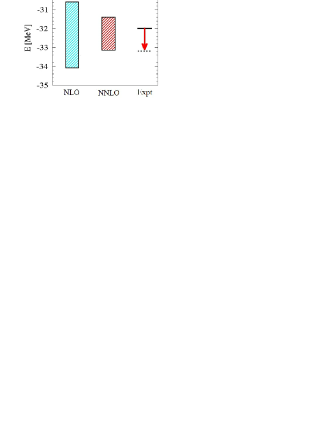
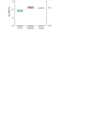
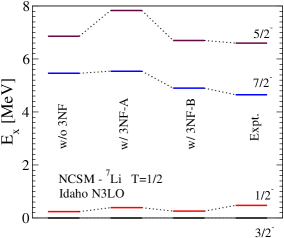
Figure 34: ⁶Li binding (left panel) and excitation (midle panel) energies at NLO and N²LO based upon the DR 2NF from [214] and the corresponding 3NF from [194] in comparison with experimental values. The bands correspond to the $\Lambda$ variation between 500 and 600 MeV. Right panel shows the results for ⁷Li based upon the N³LO Idaho 2NF combined with the N²LO 3NF (sets A and B) in comparison with experimental values. Figure courtesy of Andreas Nogga.

Let us begin with ⁶Li. In Fig. 34 we show the parameter–free results for the ⁶Li binding and excitation energies from Ref. [312] obtained within the no–core shell model framework and based upon the DR NLO and N²LO chiral forces from Ref. [214]. Going from NLO to N²LO one observes a reduction of the cut–off dependence. At N²LO, the uncertainty due to the cut–off variation is $1.8$ MeV or $5.7$% ($170$ keV or $7.6$%) of the binding (excitation) energy. Notice that for the BE, the estimated correction of the experimental value due to the missing CIB is also shown in Fig. 34. Calculation based on the N³LO Idaho NN potential [163] and N²LO 3NF led to similar results [312]. In this study, the LECs $c_{D}$ and $c_{E}$ were fixed from the ³H and ⁴He BEs which yielded two different sets: $c_{D}=-1.11$, $c_{E}=-0.66$ (3NF-A) and $c_{D}=8.14$, $c_{E}=-2.02$ (3NF-B).

We now turn to ⁷Li. Here, the only calculations performed so far are based on the N³LO Idaho NN potential augmented with the N²LO 3NF. The results for the binding energy are summarized and compared to other calculations and the experiment in Table 11 [313].

	NN	NN $+$ 3NF-A	NN $+$ 3NF-B	AV18+Urbana IX	AV18+IL2	Exp
$E_{gs}$ [MeV]	34.6	38.0	36.7	37.5	38.9	39.2
$r$ [fm]	2.40	2.19	2.31	2.33	2.25	2.27

Table 11: Comparison of the ground state binding energy results $E_{gs}$ and the point proton rms radius $r$ for ⁷Li for chiral interactions and several phenomenological combinations to the experiment.

As one can expect, ⁷Li is underbound for the NN interaction only. Both sets of 3NFs provide more binding. However, in both cases the final binding energy result is still short of the experiment by 1.2 and 2.5 MeV, respectively. This slight underbinding is encouraging in view of the general expectation that strong repulsion at short distances is required to avoid a collapse of nuclei. Clearly, we do not observe any sign of overbinding, though neither the NN force nor the 3NF have a strong repulsive core. Both interactions are very soft, yet the binding energies are reasonable. So far, it was believed that only the addition of a repulsive core, like in the Urbana-IX and Illinois models [301, 311], can cure this overbinding problem. Here, it is demonstrated that the additional structures of chiral 3NFs also prevent overbinding.

Table 11 also shows the radii obtained in this way in comparison with the experimental values and other calculations. The results for the chiral interactions are comparable to the ones based on phenomenological models Urbana-IX and Illinois. No indication is observed that soft, chiral interactions fail to saturate nuclear systems with a realistic binding energy and density.

Finally, the predictions for the excitation energies are summarized in Fig. 34. All combinations of the interactions, Idaho N³LO NN force alone, with 3NF-A or 3NF-B, do predict the right ordering for these states. The splitting of the $3/2^{-}$ and $1/2^{-}$ states is small. The agreement to experiment for 3NF-A seems to be superior. Because the splitting itself is very small, this might be accidental. More significant deviations are observed for the $7/2^{-}$ and $5/2^{-}$ states. Both, the position of this multiplet and the splitting are strongly affected by the 3NFs and the agreement with the experimental results is clearly best for 3NF-B, which is opposite to the case of BE. Clearly, further studies are needed in order to clarify the situation. As discussed before, the two N³LO NN interactions available at present use different values for the LECs $c_{i}$ which determine the strength of the 2PE 3NF. The results presented here are based on the choice of Ref. [163] and it is conceivable that the detailed description of the binding energies and spectrum is affected by the choice of $c_{i}$’s. For more details the reader is referred to [313].

To summarize, the first results for the 6N and 7N systems based on chiral forces look promising. No hard repulsive core is found to be necessary to provide realistic binding energies and densities of $p$-shell nuclei.

5 Miscellaneous omissions

In this section we give a list of related topics which were not discussed in this work. We stress that this list and the given references are not meant to be complete and should merely provide the reader some guidance to further studies.

• Electroweak and pionic probes in the nuclear environment. The exchange vector and axial–vector NN currents were considered in chiral EFT by Park, Min and Rho at one–loop level [314, 315] using the Feynman graph technique and dimensional regularization. Most of the practical applications including Compton scattering on the deuteron [316], radiative $np$ capture (at threshold) [315, 317], solar fusion [318, 319] and other solar neutrino–deuteron reactions [320, 321], hep [322] and hen [323] processes, pion–deuteron scattering at threshold [113, 324, 223], pion photo– [325, 326] and electroproduction [327], pion production in NN collisions, see [328] and references therein, and others were performed in the so–called “hybrid” approach. In such a scheme, the interaction kernel is derived within chiral EFT while the wave functions for few–nucleon initial and final states are calculated using phenomenological potentials. Certain reactions were already studied in a consistent way based on the few–nucleon wave functions obtained in chiral EFT, see e. g. Refs. [223, 329, 330, 331, 332], as well as in the pionless framework [333].

• Nuclear parity violation. A systematic study of nuclear parity–violation within the framework of effective field theory was recently carried out by Zhu et al. [334], who derived the parity–violating 1PE and 2PE potentials and discussed the ways of fixing the corresponding unknown LECs.

• Nuclear forces and the large $N_{c}$ limit. The role of the large $N_{c}$–limit of QCD for the nucleon–nucleon interaction was originally addressed in the seminal work by Witten [335] and then more recently by Kaplan et al. [336, 337]. The consistency of the large $N_{C}$–limit with the meson–exchange picture of the nuclear force is discussed in [338, 339, 340, 341].

• Chiral effective field theory and nuclear matter. Applications of chiral EFT to the nuclear many–body problem were considered by several groups, see [342, 343, 344, 345, 346] for some recent references. This is presently an active research field.

• Nucleons in (partially) quenched QCD. The NN potential in quenched and partially quenched QCD is discussed in [267]. Application of a partially–quenched extension of an effective field theory to nucleon–nucleon scattering was performed in [347]. These studies will help to relate lattice simulations in the 2N sector to experimental data.

• Low–momentum NN interaction $V_{low\;k}$. An effective interaction $V_{low\;k}$ acting in the Hilbert space of low–momentum modes was first explicitly constructed in Refs. [348, 263] using the method of unitary transformation and based on a potential of the Malfliet–Tjon type. A different method was employed in Refs. [349, 350] to construct $V_{low\;k}$ for various high–precision NN potentials. The universality of the resulting low–momentum interactions and the implications for the nuclear many–body problem are discussed in [351]. Some recent applications of $V_{low\;k}$ in the few–nucleon sector are presented in [352, 353].

6 Outlook

In this work we outlined in detail the structure of the nuclear forces in the framework of chiral effective field theory and discussed recent applications in the few–nucleon sector. We also focused on some related topics including isospin violating effects and chiral extrapolations of the two–nucleon observables.

In the future, these studies should be generalized in various ways. First, it is important to extend the N³LO analyses [162, 163] of the 2N system to few–nucleon systems which requires the derivation and numerical implementation of the corresponding N³LO contributions to the 3N and 4N forces. It remains to be seen whether the presently observed difficulties in the theoretical description of certain low–energy 3N scattering observables like e. g. the nucleon vector analyzing power $A_{y}$ can be overcome at this order in the chiral expansion. Second, the electroweak nuclear current operators should be constructed to the same accuracy as the nuclear forces and applied to a rich variety of electroweak reactions in the nuclear environment without using the “hybrid” approximation. Furthermore, given the recent theoretical progress in understanding isospin and parity–violating corrections to the nuclear force within the chiral EFT framework, a systematic study of these effects in few–nucleon systems should be pursued. In addition to these fairly straightforward extentions, a further effort is called for to achieve a better understanding of the nonperturbative renormalization in the context of the few–nucleon problem. This issue is being currently investigated by several groups. Increasing the range of applicability of the chiral EFT approach forms another challenging direction of future research. This might require the inclusion of $\Delta$–isobar as an explicit degree of freedom. One particular difficulty in such an approach is related to our lack of knowledge of the values of the corresponding LECs, since applications of the EFT with the $\Delta$’s in the single–baryon sector were not yet performed to the same detail as in the $\Delta$–less theory. Finally, it would be highly desirable to incorporate in the EFT more constraints from QCD using for example the large–$N_{c}$ expansion or lattice gauge theory.

Appendix A 2PE potential from the third order $\pi N$ amplitude

In this appendix, we give the expressions for the 2PE 2NF resulting from the diagrams which contain the third order pion–nucleon amplitude, see Fig. 7, and were obtained by Kaiser [145]. It appears to be convenient to use the (subtracted) spectral function representation:

$$V_{C,S}(q) = -\frac{2q^{6}}{\pi}\int_{2M_{\pi}}^{\infty}\,d\mu\frac{\rho_{C,S}(\mu)}{\mu^{5}(\mu^{2}+q^{2})}\,,\quad\quad V_{T}(q)=\frac{2q^{4}}{\pi}\int_{2M_{\pi}}^{\infty}\,d\mu\frac{\rho_{T}(\mu)}{\mu^{3}(\mu^{2}+q^{2})}\,,$$

$$W_{C,S}(q) = -\frac{2q^{6}}{\pi}\int_{2M_{\pi}}^{\infty}\,d\mu\frac{\eta_{C,S}(\mu)}{\mu^{5}(\mu^{2}+q^{2})}\,,\quad\quad W_{T}(q)=\frac{2q^{4}}{\pi}\int_{2M_{\pi}}^{\infty}\,d\mu\frac{\eta_{T}(\mu)}{\mu^{3}(\mu^{2}+q^{2})}\,.$$ (A.1)

For the spectral functions $\rho_{i}(\mu)$ ($\eta_{i}(\mu)$) one finds [145]:

$$\rho_{C}^{(4)}(\mu) = -\frac{3g_{A}^{4}(\mu^{2}-2M_{\pi}^{2})}{\pi\mu(4F_{\pi})^{6}}\,\theta(\tilde{\Lambda}-\mu)\,\bigg{\{}(M_{\pi}^{2}-2\mu^{2})\bigg{[}2M_{\pi}+\frac{2M_{\pi}^{2}-\mu^{2}}{2\mu}\ln\frac{\mu+2M_{\pi}}{\mu-2M_{\pi}}\bigg{]}$$

$$\mbox{\hskip 142.26378pt}+4g_{A}^{2}M_{\pi}(2M_{\pi}^{2}-\mu^{2})\bigg{\}}\,,$$

$$\eta_{S}^{(4)}(\mu) = \mu^{2}\eta_{T}^{(4)}(\mu)=-\frac{g_{A}^{4}(\mu^{2}-4M_{\pi}^{2})}{\pi(4F_{\pi})^{6}}\,\theta(\tilde{\Lambda}-\mu)\,\left\{\left(M_{\pi}^{2}-\frac{\mu^{2}}{4}\right)\ln\frac{\mu+2M_{\pi}}{\mu-2M_{\pi}}+(1+2g_{A}^{2})\mu M_{\pi}\right\}\,,$$

$$\rho_{S}^{(4)}(\mu) = \mu^{2}\rho_{T}^{(4)}(\mu)=-\theta(\tilde{\Lambda}-\mu)\,\left\{\frac{g_{A}^{2}r^{3}\mu}{8F_{\pi}^{4}\pi}(\bar{d}_{14}-\bar{d}_{15})-\frac{2g_{A}^{6}\mu r^{3}}{(8\pi F_{\pi}^{2})^{3}}\left[\frac{1}{9}-J_{1}+J_{2}\right]\right\}\,,$$

$$\eta_{C}^{(4)}(\mu) = \theta(\tilde{\Lambda}-\mu)\,\Bigg{\{}\frac{rt^{2}}{24F_{\pi}^{4}\mu\pi}\left[2(g_{A}^{2}-1)r^{2}-3g_{A}^{2}t^{2}\right](\bar{d}_{1}+\bar{d}_{2})$$ (A.2)

$${}+\frac{r^{3}}{60F_{\pi}^{4}\mu\pi}\left[6(g_{A}^{2}-1)r^{2}-5g_{A}^{2}t^{2}\right]\bar{d}_{3}-\frac{rM_{\pi}^{2}}{6F_{\pi}^{4}\mu\pi}\left[2(g_{A}^{2}-1)r^{2}-3g_{A}^{2}t^{2}\right]\bar{d}_{5}$$

$${}-\frac{1}{92160F_{\pi}^{6}\mu^{2}\pi^{3}}\Big{[}-320(1+2g_{A}^{2})^{2}M_{\pi}^{6}+240(1+6g_{A}^{2}+8g_{A}^{4})M_{\pi}^{4}\mu^{2}$$

$${}\mbox{\hskip 85.35826pt}-60g_{A}^{2}(8+15g_{A}^{2})M_{\pi}^{2}\mu^{4}+(-4+29g_{A}^{2}+122g_{A}^{4}+3g_{A}^{6})\mu^{6}\Big{]}\ln\frac{2r+\mu}{2M_{\pi}}$$

$${}-\frac{r}{2700\mu(8\pi F_{\pi}^{2})^{3}}\Big{[}-16(171+2g_{A}^{2}(1+g_{A}^{2})(327+49g_{A}^{2}))M_{\pi}^{4}+4(-73+1748g_{A}^{2}$$

$${}\mbox{\hskip 85.35826pt}+2549g_{A}^{4}+726g_{A}^{6})M_{\pi}^{2}\mu^{2}-(-64+389g_{A}^{2}+1782g_{A}^{4}+1093g_{A}^{6})\mu^{4}\Big{]}$$

$${}+\frac{2r}{3\mu(8\pi F_{\pi}^{2})^{3}}\Big{[}g_{A}^{6}t^{4}J_{1}-2g_{A}^{4}(2g_{A}^{2}-1)r^{2}t^{2}J_{2}\Big{]}\Bigg{\}}\,,$$

where we have introduced the abbreviations

$$r=\frac{1}{2}\sqrt{\mu^{2}-4M_{\pi}^{2}}\,,\quad\quad\quad t=\sqrt{\mu^{2}-2M_{\pi}^{2}}\,,$$ (A.3)

and

$$J_{n}=\int_{0}^{1}\,dx\,x^{2n-2}\,\bigg{\{}\frac{M_{\pi}^{2}}{r^{2}x^{2}}-\bigg{(}1+\frac{M_{\pi}^{2}}{r^{2}x^{2}}\bigg{)}^{3/2}\ln\frac{rx+\sqrt{M_{\pi}^{2}+r^{2}x^{2}}}{M_{\pi}}\bigg{\}}\,.$$ (A.4)

We use the scale–independent LECs $\bar{d}_{1},\;\bar{d}_{2},\;\bar{d}_{3},\;\bar{d}_{5},\;\bar{d}_{14}$ and $\bar{d}_{15}$ defined in [218]. In the limit $\tilde{\Lambda}\to\infty$ some of the integrations in Eqs. (A) with the spectral functions given in Eqs. (A) have been carried out analytically in Ref. [211].

References

- [1] H. Yukawa, Proc. Phys. Math. Soc. (Japan) 17 (1935) 48.
- [2] W. Glöckle and W. Polyzou, Few-Body Systems 9 (1990) 97.
- [3] S. Weinberg, Phys. Lett. B251 (1990) 288.
- [4] S. Weinberg, Nucl. Phys. B363 (1991) 3.
- [5] S. Weinberg, Physica A96 (1979) 327.
- [6] J. Gasser and H. Leutwyler, Ann. Phys. 158 (1984) 142.
- [7] J. Gasser and H. Leutwyler, Nucl. Phys. B250 (1985) 465.
- [8] H. Leutwyler, Phys. Lett. B374 (1996) 163, hep-ph/9601234.
- [9] P. Hasenfratz et al., Nucl. Phys. B643 (2002) 280, hep-lat/0205010.
- [10] C. Vafa and E. Witten, Nucl. Phys. B234 (1984) 173.
- [11] G. ’t Hooft, Recent developments in gauge theories., edited by G. ’t Hooft et al., Plenum New York, 1980.
- [12] S.R. Coleman and E. Witten, Phys. Rev. Lett. 45 (1980) 100.
- [13] H. Leutwyler, Ann. Phys. 235 (1994) 165, hep-ph/9311274.
- [14] S.R. Coleman, J. Wess and B. Zumino, Phys. Rev. 177 (1969) 2239.
- [15] J. Callan, Curtis G. et al., Phys. Rev. 177 (1969) 2247.
- [16] J. Gasser, Nucl. Phys. Proc. Suppl. 86 (2000) 257, hep-ph/9912548.
- [17] N.H. Fuchs, H. Sazdjian and J. Stern, Phys. Lett. B269 (1991) 183.
- [18] BNL-E865, S. Pislak et al., Phys. Rev. Lett. 87 (2001) 221801, hep-ex/0106071.
- [19] S. Pislak et al., Phys. Rev. D67 (2003) 072004, hep-ex/0301040.
- [20] J. Wess and B. Zumino, Phys. Lett. B37 (1971) 95.
- [21] E. Witten, Nucl. Phys. B223 (1983) 422.
- [22] A. Manohar and H. Georgi, Nucl. Phys. B234 (1984) 189.
- [23] J. Bijnens, G. Colangelo and G. Ecker, JHEP 02 (1999) 20, hep-ph/9902437.
- [24] J. Bijnens, G. Colangelo and G. Ecker, Annals Phys. 280 (2000) 100, hep-ph/9907333.
- [25] T. Ebertshauser, H.W. Fearing and S. Scherer, Phys. Rev. D65 (2002) 054033, hep-ph/0110261.
- [26] J. Bijnens, L. Girlanda and P. Talavera, Eur. Phys. J. C23 (2002) 539, hep-ph/0110400.
- [27] B. Ananthanarayan et al., Phys. Rept. 353 (2001) 207, hep-ph/0005297.
- [28] J. Bijnens, AIP Conf. Proc. 698 (2004) 407, hep-ph/0307082.
- [29] M. Knecht et al., Nucl. Phys. B457 (1995) 513, hep-ph/9507319.
- [30] J. Bijnens et al., Phys. Lett. B374 (1996) 210, hep-ph/9511397.
- [31] J. Bijnens et al., Nucl. Phys. B508 (1997) 263, hep-ph/9707291.
- [32] S.M. Roy, Phys. Lett. B36 (1971) 353.
- [33] G. Colangelo, J. Gasser and H. Leutwyler, Phys. Lett. B488 (2000) 261, hep-ph/0007112.
- [34] S. Weinberg, Phys. Rev. Lett. 17 (1966) 616.
- [35] G. Ecker et al., Nucl. Phys. B321 (1989) 311.
- [36] G. Ecker et al., Phys. Lett. B223 (1989) 425.
- [37] J.F. Donoghue, C. Ramirez and G. Valencia, Phys. Rev. D39 (1989) 1947.
- [38] T. Fuchs et al., Phys. Lett. B575 (2003) 11, hep-ph/0308006.
- [39] D. Djukanovic et al., Phys. Rev. Lett. 93 (2004) 122002, hep-ph/0407239.
- [40] P.C. Bruns and U.G. Meißner, Eur. Phys. J. C40 (2005) 97, hep-ph/0411223.
- [41] V. Cirigliano et al., Phys. Lett. B596 (2004) 96, hep-ph/0404004.
- [42] ALPHA, J. Heitger, R. Sommer and H. Wittig, Nucl. Phys. B588 (2000) 377, hep-lat/0006026.
- [43] UKQCD, A.C. Irving et al., Phys. Lett. B518 (2001) 243, hep-lat/0107023.
- [44] D.R. Nelson, G.T. Fleming and G.W. Kilcup, Nucl. Phys. Proc. Suppl. 106 (2002) 221, hep-lat/0110112.
- [45] G.T. Fleming, D.R. Nelson and G.W. Kilcup, Nucl. Phys. Proc. Suppl. 119 (2003) 245, hep-lat/0209141.
- [46] qq+q, F. Farchioni et al., Phys. Lett. B561 (2003) 102, hep-lat/0302011.
- [47] J. Gasser, M.E. Sainio and A. Švarc, Nucl. Phys. B307 (1988) 779.
- [48] A. Krause, Helv. Phys. Acta 63 (1990) 3.
- [49] E. Jenkins and A.V. Manohar, Phys. Lett. B255 (1991) 558.
- [50] V. Bernard et al., Nucl. Phys. B388 (1992) 315.
- [51] L.L. Foldy and S.A. Wouthuysen, Phys. Rev. 78 (1950) 29.
- [52] C. Itzykson and J.B. Zuber, Quantum Field Theory (McGraw-Hill, New-York, 1980).
- [53] T. Mannel, W. Roberts and Z. Ryzak, Nucl. Phys. B368 (1992) 204.
- [54] M.E. Luke and A.V. Manohar, Phys. Lett. B286 (1992) 348, hep-ph/9205228.
- [55] Y.Q. Chen, Phys. Lett. B317 (1993) 421.
- [56] M. Finkemeier, H. Georgi and M. McIrvin, Phys. Rev. D55 (1997) 6933, hep-ph/9701243.
- [57] J. Gasser, Ann. Phys. 136 (1981) 62.
- [58] T. Becher and H. Leutwyler, Eur. Phys. J. C9 (1999) 643, hep-ph/9901384.
- [59] H.B. Tang, (1996), hep-ph/9607436.
- [60] P.J. Ellis and H.B. Tang, Phys. Rev. C57 (1998) 3356, hep-ph/9709354.
- [61] J. Gegelia, G. Japaridze and X.Q. Wang, J. Phys. G29 (2003) 2303, hep-ph/9910260.
- [62] T. Fuchs et al., Phys. Rev. D68 (2003) 056005, hep-ph/0302117.
- [63] J. Bijnens, Int. J. Mod. Phys. A8 (1993) 3045.
- [64] V. Bernard, N. Kaiser and U.G. Meißner, Int. J. Mod. Phys. E4 (1995) 193, hep-ph/9501384.
- [65] U.G. Meißner, Rept. Prog. Phys. 56 (1993) 903, hep-ph/9302247.
- [66] A. Pich, Rept. Prog. Phys. 58 (1995) 563, hep-ph/9502366.
- [67] G. Ecker, Prog. Part. Nucl. Phys. 35 (1995) 1, hep-ph/9501357.
- [68] H. Leutwyler, Hadron Physics 94: Topics on the Structure and Interaction of Hadronic Systems, Rio Grande Do Sul, Brazil 10-14 April 1994, edited by V. Herscovitz, C. Vasconcellos and E. Ferreira, pp. 1–46, Singapore, 1995, World Scientific.
- [69] A.V. Manohar, Lectures given at 35th Int. Universitätswochen für Kern– und Teilchenphysik, Schladming, Austria, 2–9 March, 1996, hep-ph/9606222.
- [70] A.M. Bernstein, J.L. Goity and U.G. Meißner, editors, Proceedings of the 3rd Workshop on Chiral Dynamics: Theory and Experiment, Newport News, Virginia, 17–22 July, 2000, Singapore, 2002, World Scientific, hep-ph/0011140.
- [71] U.G. Meißner, H.W. Hammer and A. Wirzba, editors, Proceedings of the 4th Int. Workshop on Chiral Dynamics: Theory and Experiment, Bonn, Germany, 8–13 September, 2003, hep-ph/0311212.
- [72] S. Scherer, Adv. Nucl. Phys. 27 (2002) 277, hep-ph/0210398.
- [73] M. Lutz, hep-ph/9606301.
- [74] U. van Kolck, Nucl. Phys. A645 (1999) 273, nucl-th/9808007.
- [75] D.B. Kaplan, M.J. Savage and M.B. Wise, Phys. Lett. B424 (1998) 390, nucl-th/9801034.
- [76] D.B. Kaplan, M.J. Savage and M.B. Wise, Nucl. Phys. B534 (1998) 329, nucl-th/9802075.
- [77] J. Gegelia, nucl-th/9802038.
- [78] J.W. Chen, G. Rupak and M.J. Savage, Nucl. Phys. A653 (1999) 386, nucl-th/9902056.
- [79] D.B. Kaplan, Nucl. Phys. B494 (1997) 471, nucl-th/9610052.
- [80] P.F. Bedaque, H.W. Hammer and U. van Kolck, Nucl. Phys. A646 (1999) 444, nucl-th/9811046.
- [81] P.F. Bedaque, H.W. Hammer and U. van Kolck, Phys. Rev. Lett. 82 (1999) 463, nucl-th/9809025.
- [82] P.F. Bedaque, H.W. Hammer and U. van Kolck, Nucl. Phys. A676 (2000) 357, nucl-th/9906032.
- [83] F. Gabbiani, P.F. Bedaque and H.W. Griesshammer, Nucl. Phys. A675 (2000) 601, nucl-th/9911034.
- [84] P.F. Bedaque et al., Nucl. Phys. A714 (2003) 589, nucl-th/0207034.
- [85] B. Blankleider and J. Gegelia, AIP Conf. Proc. 603 (2001) 233, nucl-th/0107043.
- [86] I.R. Afnan and D.R. Phillips, Phys. Rev. C69 (2004) 034010, nucl-th/0312021.
- [87] H.W. Griesshammer, Nucl. Phys. A744 (2004) 192, nucl-th/0404073.
- [88] E. Braaten and H.W. Hammer, (2004), cond-mat/0410417.
- [89] G.V. Skorniakov and K.A. Ter-Martirosian, Sov. Phys. JETP 4 (1957) 648.
- [90] G.S. Danilov, Sov. Phys. JETP 13 (1961) 349.
- [91] V.F. Kharchenko, Sov. J. Nucl. Phys. 16 (1973) 173.
- [92] B. Blankleider and J. Gegelia, (2000), nucl-th/0009007.
- [93] V. Efimov, Phys. Rev. C 44 (1991) 2303.
- [94] S.R. Beane et al., nucl-th/0008064.
- [95] P.F. Bedaque and U. van Kolck, Ann. Rev. Nucl. Part. Sci. 52 (2002) 339, nucl-th/0203055.
- [96] U. van Kolck, (2004), nucl-th/0409064.
- [97] V. Efimov, Nucl. Phys. A 362 (1981) 45, Erratum ibid. A378 (1982) 581.
- [98] L. Platter, H.W. Hammer and U.G. Meißner, Phys. Rev. A70 (2004) 052101, cond-mat/0404313.
- [99] L. Platter, H.W. Hammer and U.G. Meißner, Phys. Lett. B607 (2005) 254, nucl-th/0409040.
- [100] M. Lutz, Nucl. Phys. A677 (2000) 241, nucl-th/9906028.
- [101] S. Fleming, T. Mehen and I.W. Stewart, Nucl. Phys. A677 (2000) 313, nucl-th/9911001.
- [102] T.D. Cohen and J.M. Hansen, Phys. Rev. C59 (1999) 13, nucl-th/9808038.
- [103] T.D. Cohen and J.M. Hansen, Phys. Rev. C59 (1999) 3047, nucl-th/9901065.
- [104] J. Gegelia, nucl-th/9806028.
- [105] J.V. Steele and R.J. Furnstahl, Nucl. Phys. A645 (1999) 439, nucl-th/9808022.
- [106] D.B. Kaplan and J.V. Steele, Phys. Rev. C60 (1999) 064002, nucl-th/9905027.
- [107] G. Rupak and N. Shoresh, Phys. Rev. C60 (1999) 054004, nucl-th/9902077.
- [108] V.G.J. Stoks et al., Phys. Rev. C48 (1993) 792.
- [109] NN-Online program, M. C. M. Rentmeester et al., http://nn-online.org.
- [110] S.S. Schweber, An introduction to relativistic quantum field theory (Harper and Row, New York, Evanston & London, 1966).
- [111] M. Gell-Mann and M.L. Goldberger, Phys. Rev. 96 (1954) 1433.
- [112] S. Weinberg, The quantum theory of fields, Vol. 1 (Cambridge University Press, Cambridge, U.K., 1995).
- [113] S. Weinberg, Phys. Lett. B295 (1992) 114, hep-ph/9209257.
- [114] S.R. Beane et al., Nucl. Phys. A700 (2002) 377, nucl-th/0104030.
- [115] J. Gegelia and S. Scherer, nucl-th/0403052.
- [116] A. Nogga, R.G.E. Timmermans and U. van Kolck, nucl-th/0506005.
- [117] M.C. Birse, nucl-th/0507077.
- [118] J.L. Friar, Mod. Phys. Lett. A11 (1996) 3043, nucl-th/9601013.
- [119] C. Ordóñez, L. Ray and U. van Kolck, Phys. Rev. C53 (1996) 2086, hep-ph/9511380.
- [120] N. Fettes and U.G. Meißner, Nucl. Phys. A693 (2001) 693, hep-ph/0101030.
- [121] U.L. van Kolck, Soft physics: Applications of effective chiral lagrangians to nuclear physics and quark models, PhD thesis, University of Texas, Austin, USA, 1993, UMI-94-01021.
- [122] S. Steininger, Reelle und virtuelle photonen in chiraler Störungstheorie, PhD thesis, University Bonn, Germany, 1999.
- [123] N. Fettes et al., Ann. Phys. 283 (2000) 273, hep-ph/0001308.
- [124] J. Gasser et al., Eur. Phys. J. C26 (2002) 13, hep-ph/0206068.
- [125] E. Epelbaum and U.G. Meißner, Phys. Rev. C (to appear), nucl-th/0502052.
- [126] R.J.N. Phillips, Reports on Progress in Physics XXII (1959) 562.
- [127] I. Tamm, J. Phys. (USSR) 9 (1945) 449.
- [128] S.M. Dancoff, Phys. Rev. 78 (1950) 382.
- [129] S. Okubo, Prog. Theor. Phys. (Japan) 12 (1954) 603.
- [130] N. Fukuda, K. Sawada and M. Taketani, Prog. Theor. Phys. (Japan) 12 (1954) 156.
- [131] E. Epelbaum, W. Glöckle and U.G. Meißner, Nucl. Phys. A637 (1998) 107, nucl-th/9801064.
- [132] E. Epelbaum, The nucleon nucleon interaction in a chiral effective field theory, PhD thesis, Ruhr–University Bochum, Germany, 2000, JUL-3803.
- [133] H. Krebs, V. Bernard and U.G. Meißner, Ann. Phys. 316 (2005) 160, nucl-th/0407078.
- [134] E. Epelbaum, U.G. Meißner and W. Glöckle, Nucl. Phys. A714 (2003) 535, nucl-th/0207089.
- [135] O.W. Greenberg and S.S. Schweber, Nuovo Cim. 8 (1958) 378.
- [136] L.D. Faddeev, Dokl. Akad. Nauk SSSR 152 (1963) 573.
- [137] V.A. Fateev and A.S. Shvarts, Sov. Phys. Dokl. 18 (1973) 165.
- [138] A.V. Shebeko and M.I. Shirokov, Phys. Part. Nucl. 32 (2001) 15, nucl-th/0102037.
- [139] E. Epelbaum, W. Glöckle and U.G. Meißner, Nucl. Phys. A671 (2000) 295, nucl-th/9910064.
- [140] J.L. Friar and S.A. Coon, Phys. Rev. C49 (1994) 1272.
- [141] J.L. Friar, Annals Phys. 104 (1977) 380.
- [142] N. Kaiser, R. Brockmann and W. Weise, Nucl. Phys. A625 (1997) 758, nucl-th/9706045.
- [143] N. Kaiser, Phys. Rev. C61 (2000) 014003, nucl-th/9910044.
- [144] N. Kaiser, Phys. Rev. C62 (2000) 024001, nucl-th/9912054.
- [145] N. Kaiser, Phys. Rev. C64 (2001) 057001, nucl-th/0107064.
- [146] J.L. Friar, Phys. Rev. C60 (1999) 034002, nucl-th/9901082.
- [147] E. Epelbaum, W. Glöckle and U.G. Meißner, Eur. Phys. J. A19 (2004) 125, nucl-th/0304037.
- [148] J.F. Donoghue and B.R. Holstein, Phys. Lett. B436 (1998) 331.
- [149] J.F. Donoghue, B.R. Holstein and B. Borasoy, Phys. Rev. D59 (1999) 036002, hep-ph/9804281.
- [150] B. Borasoy et al., Phys. Rev. D66 (2002) 094020, hep-ph/0210092.
- [151] D.B. Leinweber, A.W. Thomas and R.D. Young, Phys. Rev. Lett. 92 (2004) 242002, hep-lat/0302020.
- [152] V. Bernard, T.R. Hemmert and U.G. Meißner, Nucl. Phys. A732 (2004) 149, hep-ph/0307115.
- [153] M. Frink, U.G. Meißner and I. Scheller, Eur. Phys. J. A24 (2005) 395, hep-lat/0501024.
- [154] P. Büttiker and U.G. Meißner, Nucl. Phys. A668 (2000) 97, hep-ph/9908247.
- [155] R. Machleidt, K. Holinde and C. Elster, Phys. Rept. 149 (1987) 1.
- [156] M.R. Robilotta and C.A. da Rocha, Nucl. Phys. A615 (1997) 391, nucl-th/9611056.
- [157] M. Taketani, S. Mashida and S. O-Numa, Prog. Theor. Phys. (Japan) 7 (1952) 45.
- [158] K.A. Brueckener and K.M. Watson, Phys. Rev. 92 (1953) 1023.
- [159] H. Sugawara and S. Okubo, Phys. Rev. 117 (1960) 605.
- [160] H. Sugawara and F. Von Hippel, Phys. Rev. 172 (1968) 1764.
- [161] J.C. Pupin and M.R. Robilotta, Phys. Rev. C60 (1999) 014003, nucl-th/9903028.
- [162] E. Epelbaum, W. Glöckle and U.G. Meißner, Nucl. Phys. A747 (2005) 362, nucl-th/0405048.
- [163] D.R. Entem and R. Machleidt, Phys. Rev. C68 (2003) 041001, nucl-th/0304018.
- [164] N. Kaiser, Phys. Rev. C63 (2001) 044010, nucl-th/0101052.
- [165] N. Kaiser, Phys. Rev. C65 (2002) 017001, nucl-th/0109071.
- [166] H. Kamada and W. Glöckle, Phys. Rev. Lett. 80 (1998) 2547, nucl-th/9903071.
- [167] R. Urech, Nucl. Phys. B433 (1995) 234.
- [168] U.G. Meißner, G. Müller and S. Steininger, Phys. Lett. B406 (1997) 154, hep-ph/9704377, erratum ibid. B407 (1997) 454.
- [169] U.G. Meißner and S. Steininger, Phys. Lett. B419 (1998) 403, hep-ph/9709453.
- [170] G. Müller and U.G. Meißner, Nucl. Phys. B556 (1999) 265, hep-ph/9903375.
- [171] U. van Kolck, Few Body Syst. Suppl. 9 (1995) 444.
- [172] U. van Kolck, J.L. Friar and T. Goldman, Phys. Lett. B371 (1996) 169, nucl-th/9601009.
- [173] J.L. Friar and U. van Kolck, Phys. Rev. C60 (1999) 034006, nucl-th/9906048.
- [174] J.L. Friar et al., Phys. Rev. C68 (2003) 024003, nucl-th/0303058.
- [175] J.L. Friar et al., Phys. Rev. C70 (2004) 044001, nucl-th/0406026.
- [176] E.M. Henley and G.A. Miller, Mesons and nuclei, edited by M. Rho and D.H. Wilkinson, volume 1, p. 405, Amsterdam, 1979, North–Holland.
- [177] G.J.M. Austin and J.J. de Swart, Phys. Rev. Lett. 50 (1983) 2039.
- [178] E.A. Ueling, Phys. Rev. 48 (1935) 55.
- [179] L. Durand III, Phys. Rev. 108 (1957) 1597.
- [180] V.G. Stoks, The magnetic moment interaction in NN phase shift analysis, PhD thesis, University Nijmegen, The Netherlands, 1990.
- [181] U. van Kolck et al., Phys. Rev. Lett. 80 (1998) 4386, nucl-th/9710067.
- [182] J.A. Niskanen, Phys. Rev. C65 (2002) 037001, nucl-th/0108015.
- [183] S.A. Coon and J.A. Niskanen, Phys. Rev. C53 (1996) 1154.
- [184] J. Gasser and H. Leutwyler, Phys. Rept. 87 (1982) 77.
- [185] M.R. Robilotta, Phys. Rev. C63 (2001) 044004, nucl-th/0009001.
- [186] R. Higa, nucl-th/0411046.
- [187] R. Higa and M.R. Robilotta, Phys. Rev. C68 (2003) 024004, nucl-th/0304025.
- [188] R. Higa, M.R. Robilotta and C.A. da Rocha, Phys. Rev. C69 (2004) 034009, nucl-th/0310011.
- [189] S.A. Coon and J.L. Friar, Phys. Rev. C34 (1986) 1060.
- [190] J.A. Eden and M.F. Gari, Phys. Rev. C53 (1996) 1510, nucl-th/9601025.
- [191] S.N. Yang and W. Glöckle, Phys. Rev. C33 (1986) 1774.
- [192] U. van Kolck, Phys. Rev. C49 (1994) 2932.
- [193] J.L. Friar, D. Huber and U. van Kolck, Phys. Rev. C59 (1999) 53, nucl-th/9809065.
- [194] E. Epelbaum et al., Phys. Rev. C66 (2002) 064001, nucl-th/0208023.
- [195] E. Epelbaum, U.G. Meißner and J.E. Palomar, Phys. Rev. C71 (2005) 024001, nucl-th/0407037.
- [196] E. Epelbaum, nucl-th/0412003.
- [197] J.L. Friar, G.L. Payne and U. van Kolck, Phys. Rev. C71 (2005) 024003, nucl-th/0408033.
- [198] S.N. Yang, Phys. Rev. C19 (1979) 1114.
- [199] S.N. Yang, J. Phys. G9 (1983) L115.
- [200] E. Jenkins and A.V. Manohar, Phys. Lett. B259 (1991) 353.
- [201] T.R. Hemmert, B.R. Holstein and J. Kambor, J. Phys. G24 (1998) 1831, hep-ph/9712496.
- [202] V. Pascalutsa and D.R. Phillips, Phys. Rev. C67 (2003) 055202, nucl-th/0212024.
- [203] V. Bernard, N. Kaiser and U.G. Meißner, Nucl. Phys. A615 (1997) 483, hep-ph/9611253.
- [204] T. Ericson and W. Weise, Pions and Nuclei (Clarendon, Oxford, U.K., 1988).
- [205] N. Kaiser, S. Gerstendorfer and W. Weise, Nucl. Phys. A637 (1998) 395, nucl-th/9802071.
- [206] V.R. Pandharipande, D.R. Phillips and U. van Kolck, nucl-th/0501061.
- [207] N. Fettes and U.G. Meißner, Nucl. Phys. A679 (2001) 629, hep-ph/0006299.
- [208] V. Pascalutsa, Phys. Rev. D58 (1998) 096002, hep-ph/9802288.
- [209] V. Bernard, T.R. Hemmert and U.G. Meißner, Phys. Lett. B565 (2003) 137, hep-ph/0303198.
- [210] V. Bernard, T.R. Hemmert and U.G. Meißner, Phys. Lett. B622 (2005) 141, hep-lat/0503022.
- [211] D.R. Entem and R. Machleidt, Phys. Rev. C66 (2002) 014002, nucl-th/0202039.
- [212] M.C. Birse and J.A. McGovern, Phys. Rev. C70 (2004) 054002, nucl-th/0307050.
- [213] J.L. Ballot, M.R. Robilotta and C.A. da Rocha, Phys. Rev. C57 (1998) 1574, nucl-th/9801022.
- [214] E. Epelbaum et al., Eur. Phys. J. A15 (2002) 543, nucl-th/0201064.
- [215] H.P. Stapp, T.J. Ypsilantis and N. Metropolis, Phys. Rev. 105 (1957) 302.
- [216] M. Mojžiš, Eur. Phys. J. C2 (1998) 181, hep-ph/9704415.
- [217] V. Bernard, N. Kaiser and U.G. Meißner, Nucl. Phys. B457 (1995) 147, hep-ph/9507418.
- [218] N. Fettes, U.G. Meißner and S. Steininger, Nucl. Phys. A640 (1998) 199, hep-ph/9803266.
- [219] M.C.M. Rentmeester et al., Phys. Rev. Lett. 82 (1999) 4992, nucl-th/9901054.
- [220] M.C.M. Rentmeester, R.G.E. Timmermans and J.J. de Swart, Phys. Rev. C67 (2003) 044001, nucl-th/0302080.
- [221] D.R. Entem and R. Machleidt, (2003), nucl-th/0303017.
- [222] SAID on-line program, R. A.Arndt et al., http://gwdac.phys.gwu.edu.
- [223] S.R. Beane et al., Nucl. Phys. A720 (2003) 399, hep-ph/0206219.
- [224] K.G. Richardson, Chiral symmetry and the nucleon nucleon interaction, PhD thesis, University of Manchester, 1999, hep-ph/0008118.
- [225] J. Gegelia, J. Phys. G25 (1999) 1681, nucl-th/9805008.
- [226] T. Frederico, V.S. Timoteo and L. Tomio, Nucl. Phys. A653 (1999) 209, nucl-th/9902052.
- [227] D.R. Phillips, I.R. Afnan and A.G. Henry-Edwards, Phys. Rev. C61 (2000) 044002, nucl-th/9910063.
- [228] J. Gegelia and G. Japaridze, Phys. Lett. B517 (2001) 476, nucl-th/0108005.
- [229] S.R. Beane, T.D. Cohen and D.R. Phillips, Nucl. Phys. A632 (1998) 445, nucl-th/9709062.
- [230] D.R. Phillips, S.R. Beane and T.D. Cohen, Annals Phys. 263 (1998) 255, hep-th/9706070.
- [231] M.C. Birse, J.A. McGovern and K.G. Richardson, Phys. Lett. B464 (1999) 169, hep-ph/9807302.
- [232] T.D. Cohen and J.M. Hansen, Phys. Lett. B440 (1998) 233, nucl-th/9808006.
- [233] D.R. Phillips, S.R. Beane and M.C. Birse, J. Phys. A32 (1999) 3397, hep-th/9810049.
- [234] J.F. Yang, (2004), nucl-th/0407090.
- [235] J.F. Yang and J.H. Huang, Phys. Rev. C71 (2005) 034001, nucl-th/0409023.
- [236] K.G. Wilson, Phys. Rev. B4 (1971) 3174,3184.
- [237] G.P. Lepage, How to renormalize the Schrödinger equation, talk given at the INT program Effective Field Theories and Effective Interactions, INT, Seattle, USA, June 25–August 2, 2000.
- [238] G.P. Lepage, nucl-th/9706029.
- [239] S.R. Beane et al., Phys. Rev. A64 (2001) 042103, quant-ph/0010073.
- [240] M. Pavon Valderrama and E. Ruiz Arriola, Phys. Lett. B580 (2004) 149, nucl-th/0306069.
- [241] M. Pavon Valderrama and E. Ruiz Arriola, Phys. Rev. C70 (2004) 044006, nucl-th/0405057.
- [242] M. Pavon Valderrama and E. Ruiz Arriola, nucl-th/0504067.
- [243] M. Pavon Valderrama and E. Ruiz Arriola, nucl-th/0507075.
- [244] D. Djukanovic et al., hep-ph/0407170.
- [245] A.A. Slavnov, Nucl. Phys. B31 (1971) 301.
- [246] T.S. Park et al., Nucl. Phys. A646 (1999) 83, nucl-th/9807054.
- [247] D.R. Entem and R. Machleidt, Phys. Lett. B524 (2002) 93, nucl-th/0108057.
- [248] E. Epelbaum, W. Glöckle and U.G. Meißner, Eur. Phys. J. A19 (2004) 401, nucl-th/0308010.
- [249] M. Walzl, U.G. Meißner and E. Epelbaum, Nucl. Phys. A693 (2001) 663, nucl-th/0010019.
- [250] R. Machleidt, private communication.
- [251] J.R. Bergervoet et al., Phys. Rev. C41 (1990) 1435.
- [252] J.J. de Swart, C.P.F. Terheggen and V.G.J. Stoks, (1995), nucl-th/9509032.
- [253] J.L. Friar, J. Martorell and D.W.L. Sprung, Phys. Rev. A56 (1997) 4579, nucl-th/9707016.
- [254] M.C.M. Rentmeester, private communication.
- [255] V. van der Leun and C. Alderlisten, Nucl. Phys. A380 (1982) 261.
- [256] D.M. Bishop and L.M. Cheung, Phys. Rev. A20 (1979) 381.
- [257] T.E.O. Ericson and M. Rosa-Clot, Phys. Rev. A405 (1983) 497.
- [258] N.L. Rodning and L.D. Knutson, Phys. Rev. C41 (1990) 898.
- [259] R. Machleidt and D.R. Entem, nucl-th/0503025.
- [260] E. Epelbaum et al., Phys. Rev. C65 (2002) 044001, nucl-th/0106007.
- [261] R. Machleidt, Adv. Nucl. Phys. 19 (1989) 189.
- [262] V.G.J. Stoks et al., Phys. Rev. C49 (1994) 2950, nucl-th/9406039.
- [263] E. Epelbaum et al., Nucl. Phys. A645 (1999) 413, nucl-th/9809084.
- [264] M. Fukugita et al., Phys. Rev. D52 (1995) 3003, hep-lat/9501024.
- [265] S.R. Beane and M.J. Savage, Nucl. Phys. A713 (2003) 148, hep-ph/0206113.
- [266] A. Bulgac, G.A. Miller and M. Strikman, Phys. Rev. C56 (1997) 3307, nucl-th/9708045.
- [267] S.R. Beane and M.J. Savage, Phys. Lett. B535 (2002) 177, hep-lat/0202013.
- [268] S.R. Beane and M.J. Savage, Nucl. Phys. A717 (2003) 91, nucl-th/0208021.
- [269] E. Epelbaum, U.G. Meißner and W. Glöckle, (2002), nucl-th/0208040.
- [270] N. Fettes, V. Bernard and U.G. Meißner, Nucl. Phys. A669 (2000) 269, hep-ph/9907276.
- [271] N. Fettes, Pion–Nucleon Physics in Chiral Perturbation Theory, PhD thesis, Universität Bonn, Germany, 2000, JUL-3814.
- [272] E. Matsinos, (1998), hep-ph/9807395.
- [273] E. Epelbaum, W. Glöckle and U.G. Meißner, Nuclear Many–Body and Medium Effects in Nuclear Interactions and Reactions, edited by K. Hatanaka et al., p. 99, Singapore, 2002, World Scientific.
- [274] S.R. Beane, Nucl. Phys. B695 (2004) 192, hep-lat/0403030.
- [275] T.R. Hemmert, M. Procura and W. Weise, Phys. Rev. D68 (2003) 075009, hep-lat/0303002.
- [276] E. Braaten and H.W. Hammer, Phys. Rev. Lett. 91 (2003) 102002, nucl-th/0303038.
- [277] E. Epelbaum et al., Phys. Rev. Lett. 86 (2001) 4787, nucl-th/0007057.
- [278] D.R. Entem, R. Machleidt and H. Witała, Phys. Rev. C65 (2002) 064005, nucl-th/0111033.
- [279] E. Epelbaum et al., in preparation.
- [280] K. Ermisch et al., Phys. Rev. C68 (2003) 051001, nucl-ex/0308012.
- [281] K. Ermisch et al., Phys. Rev. C71 (2005) 064004.
- [282] C. Duweke et al., Phys. Rev. C71 (2005) 054003, nucl-ex/0412024.
- [283] S. Kistryn et al., Phys. Rev. C (to appear), nucl-ex/0508012.
- [284] H. Witała et al., in preparation.
- [285] W. Glöckle et al., Phys. Rept. 274 (1996) 107.
- [286] H. Kamada and W. Glöckle, Nucl. Phys. A548 (1992) 205.
- [287] A. Nogga et al., Phys. Lett. B409 (1997) 19.
- [288] D. Hüber et al., Acta Phys. Polon. B28 (1997) 1677, nucl-th/9611007.
- [289] W. Glöckle, The Quantum Mechanical Few-Body Problem (Springer-Verlag, Berlin, 1983).
- [290] H. Witała, T. Cornelius and W. Glöckle, Few-Body Systems 3 (1988) 123.
- [291] D. Hüber et al., Few Body Syst. 22 (1997) 107, nucl-th/9611021.
- [292] A. Nogga, H. Kamada and W. Glöckle, Phys. Rev. Lett. 85 (2000) 944.
- [293] A. Nogga et al., Phys. Rev. Lett. 85 (2000) 944.
- [294] A. Kievsky, private communication.
- [295] R.B. Wiringa, V.G.J. Stoks and R. Schiavilla, Phys. Rev. C51 (1995) 38, nucl-th/9408016.
- [296] W. Dilg, L. Koester and W. Nistler, Phys.Lett. B36 (1971) 208.
- [297] T.C. Black et al., Phys. Rev. Lett. 90 (2003) 192502, nucl-ex/0305019.
- [298] Y. Koike and J. Haidenbauer, Nucl. Phys. A463 (1987) 365c.
- [299] H. Witała, D. Hüber and W. Glöckle, Phys. Rev. C49 (1994) R14.
- [300] S.A. Coon and H.K. Han, Few Body Syst. 30 (2001) 131, nucl-th/0101003.
- [301] B.S. Pudliner et al., Phys. Rev. C56 (1997) 1720, nucl-th/9705009.
- [302] A. Kievsky, Phys. Rev. C60 (1999) 034001, nucl-th/9905045.
- [303] D. Hüber et al., Few Body Syst. 30 (2001) 95, nucl-th/9910034.
- [304] C.R. Howell et al., Nucl. Phys. A631 (1998) 692c.
- [305] J. Zejma et al., Phys. Rev. C55 (1997) 42.
- [306] J. Kuroś-Żołnierczuk et al., Phys. Rev. C66 (2002) 024004, nucl-th/0203020.
- [307] J.A. Tjon, Phys. Lett. B56 (1975) 217.
- [308] A. Nogga et al., Phys. Rev. C65 (2002) 054003, nucl-th/0112026.
- [309] S.C. Pieper and R.B. Wiringa, Ann. Rev. Nucl. Part. Sci. 51 (2001) 53, nucl-th/0103005.
- [310] P. Navrátil and W.E. Ormand, Phys. Rev. C68 (2003) 034305, nucl-th/0305090.
- [311] S.C. Pieper et al., Phys. Rev. C64 (2001) 014001, nucl-th/0102004.
- [312] A. Nogga et al., Nucl. Phys. A737 (2004) 236.
- [313] A. Nogga et al., in preparation.
- [314] T.S. Park, D.P. Min and M. Rho, Phys. Rept. 233 (1993) 341, hep-ph/9301295.
- [315] T.S. Park, D.P. Min and M. Rho, Nucl. Phys. A596 (1996) 515, nucl-th/9505017.
- [316] S.R. Beane et al., Nucl. Phys. A747 (2005) 311, nucl-th/0403088.
- [317] T.S. Park et al., Phys. Lett. B472 (2000) 232, nucl-th/9906005.
- [318] T.S. Park et al., Astrophys. J. 507 (1998) 443, astro-ph/9804144.
- [319] T.S. Park et al., nucl-th/0106025.
- [320] S. Ando et al., Phys. Lett. B533 (2002) 25, nucl-th/0109053.
- [321] S. Ando et al., Phys. Lett. B555 (2003) 49, nucl-th/0206001.
- [322] T.S. Park et al., Phys. Rev. C67 (2003) 055206, nucl-th/0208055.
- [323] S.C. Park and J.h. Song, (2003), hep-ph/0306112.
- [324] S.R. Beane et al., Phys. Rev. C57 (1998) 424, nucl-th/9708035.
- [325] S.R. Beane et al., Nucl. Phys. A618 (1997) 381, hep-ph/9702226.
- [326] V. Lensky et al., nucl-th/0505039.
- [327] V. Bernard, H. Krebs and U.G. Meißner, Phys. Rev. C61 (2000) 058201, nucl-th/9912033.
- [328] C. Hanhart, Phys. Rept. 397 (2004) 155, hep-ph/0311341.
- [329] M. Walzl and U.G. Meißner, Phys. Lett. B513 (2001) 37, nucl-th/0103020.
- [330] H. Krebs, V. Bernard and U.G. Meißner, Nucl. Phys. A713 (2003) 405, nucl-th/0207072.
- [331] D.R. Phillips, nucl-th/0503044.
- [332] H. Krebs, V. Bernard and U.G. Meißner, Eur. Phys. J. A22 (2004) 503, nucl-th/0405006.
- [333] U.G. Meißner, U. Raha and A. Rusetsky, Eur. Phys. J. C41 (2005) 213, nucl-th/0501073.
- [334] S.L. Zhu et al., Nucl. Phys. A748 (2005) 435, nucl-th/0407087.
- [335] E. Witten, Nucl. Phys. B160 (1979) 57.
- [336] D.B. Kaplan and M.J. Savage, Phys. Lett. B365 (1996) 244, hep-ph/9509371.
- [337] D.B. Kaplan and A.V. Manohar, Phys. Rev. C56 (1997) 76, nucl-th/9612021.
- [338] M.K. Banerjee, T.D. Cohen and B.A. Gelman, Phys. Rev. C65 (2002) 034011, hep-ph/0109274.
- [339] T.D. Cohen and B.A. Gelman, Phys. Lett. B540 (2002) 227, nucl-th/0202036.
- [340] A.V. Belitsky and T.D. Cohen, Phys. Rev. C65 (2002) 064008, hep-ph/0202153.
- [341] T.D. Cohen, Phys. Rev. C66 (2002) 064003, nucl-th/0209072.
- [342] J.A. Oller, Phys. Rev. C65 (2002) 025204, hep-ph/0101204.
- [343] U.G. Meißner, J.A. Oller and A. Wirzba, Annals Phys. 297 (2002) 27, nucl-th/0109026.
- [344] L. Girlanda, A. Rusetsky and W. Weise, Annals Phys. 312 (2004) 92, hep-ph/0311128.
- [345] D. Vretenar and W. Weise, Lect. Notes Phys. 641 (2004) 65, nucl-th/0312022.
- [346] R.J. Furnstahl, Int. J. Mod. Phys. B17 (2003) 5111, nucl-th/0109007.
- [347] S.R. Beane and M.J. Savage, Phys. Rev. D67 (2003) 054502, hep-lat/0210046.
- [348] E. Epelbaum, W. Glöckle and U.G. Meißner, Phys. Lett. B439 (1998) 1, nucl-th/9804005.
- [349] S.K. Bogner et al., Phys. Lett. B576 (2003) 265, nucl-th/0108041.
- [350] S. Bogner, T.T.S. Kuo and L. Coraggio, Nucl. Phys. A684 (2001) 432, nucl-th/0204058.
- [351] S.K. Bogner, T.T.S. Kuo and A. Schwenk, Phys. Rept. 386 (2003) 1, nucl-th/0305035.
- [352] S. Fujii et al., Phys. Rev. C70 (2004) 024003, nucl-th/0404049.
- [353] A. Nogga, S.K. Bogner and A. Schwenk, Phys. Rev. C70 (2004) 061002, nucl-th/0405016.