Nuclear Symmetry Energy in Relativistic Mean Field Theory

Abstract

The physical origin of the nuclear symmetry energy is studied within the relativistic mean field (RMF) theory. Based on the nuclear binding energies calculated with and without mean isovector potential for several isobaric chains we confirm earlier Skyrme-Hartree-Fock result that the nuclear symmetry energy strength depends on the mean level spacing $\varepsilon(A)$ and an effective mean isovector potential strength $\kappa(A)$. A detailed analysis of the isospin dependence of the two components contributing to the nuclear symmetry energy reveals a quadratic dependence due to the mean-isoscalar potential, $\sim$ $\varepsilon\,T^{2}$, and, completely unexpectedly, the presence of a strong linear component $\sim$ $\kappa\,T(T+1+\varepsilon/\kappa)$ in the isovector potential. The latter generates a nuclear symmetry energy in RMF theory that is proportional to $E_{\text{sym}}\sim T(T+1)$ at variance to the non-relativistic calculation. The origin of the linear term in RMF theory needs to be further explored.

One of the most important topics in current nuclear physics is to search for the existence limit of atomic nuclei, i.e., to determine the nuclear drip line. In this respect, the role of the continuum in loosely bound nuclei and, in particular, its impact on the treatment of pairing correlations has been discussed to great extent in recent time. However, the proper understanding and correct reproduction of the nuclear symmetry energy (NSE) may have even greater bearing for masses of loosely bound nuclei and certainly is a key issue in the study of exotic nuclei. The very fundamental questions in this respect concern both the understanding of the microscopic origin of the NSE strength as well as its isospin dependence. The latter issue has attracted recently great attention also in $N\sim Z$ nuclei, see Ref. [Sat01x] and references therein.

The NSE is conventionally parametrized as:

$$E_{\text{sym}}=a_{\text{sym}}(A)T(T+\lambda)$$ (1)

where $T=|T_{z}|=|N-Z|/2$. The strength of the NSE admits typically volume and surface components $a_{\text{sym}}(A)=a_{\text{v}}/A-a_{\text{s}}/A^{4/3}$ and its physical origin is traditionally explained in terms of the kinetic energy and mean isovector potential (interaction) contributions i.e. $a_{\text{sym}}(A)a_{\text{kin}}(A)+a_{\text{int}}(A)$, respectively [Boh69] . The linear term is found to be strongly model dependent and there is a common belief that mean-field models yield essentially only a quadratic term $\lambda\approx 0$. On the other hand, the nuclear shell-model [Tal56] ; [Tal62] ; [Zel96] or models restoring isospin symmetry [Nee02x] suggest that $\lambda\approx 1$. No consensus is reached so far concerning the value of $\lambda$ although there is certain preference for $\lambda\approx 1$. Indeed, experimental masses of nuclei with small values of $T$ supports the existence of the linear term [Mye66] . Similar conclusions were reached by Jänecke et al. [Jan65x] based on the analysis of experimental binding energies for $A<80$ nuclei. One of the most accurate mass formula, the so called FRDM  [Mol95] employs a value of $\lambda\approx 1$ but inconsistently admits only a volume-like linear term. Assuming $T(T+1)$ dependence Duflo and Zuker have performed a global fit to nuclear masses obtaining [Duf95]

$$a_{\text{sym}}(A)=\frac{134.4}{A}-\frac{203.6}{A^{4/3}}~{}\text{[MeV]}.$$ (2)

A different view on the origin of the NSE was presented recently by Satuła and Wyss. In Refs. [Sat03] ; [Glo04] ; [Sat05] it was demonstrated using the Skyrme-Hartree-Fock (SHF) model that the NSE can be directly associated with the mean level spacing $\varepsilon(A)$ and mean isovector potential, $E_{\text{sym}}\dfrac{1}{2}\varepsilon(A)T^{2}+\dfrac{1}{2}\kappa(A)T(T+1)$ [Sat03] ; [Glo04] ; [Sat05] . Surprisingly, the self-consistent calculations revealed that the complicated isovector mean potential induced by the Skyrme force is similar to that obtained from a simple interaction $\dfrac{1}{2}\kappa(A)\hat{\bf T}\cdot\hat{\bf T}$, i.e., is very accurately characterized by a single strength $\kappa(A)$ [Sat03] ; [Glo04] ; [Sat05] . This study revealed also that the SHF theory yield in fact a (partial) linear term with $\lambda\approx\kappa/(2a_{\text{sym}})$ and that this term originates from neutron-proton exchange interaction.

Alongside with the SHF calculation, the relativistic mean field (RMF) theory has been used for a large variety of nuclear structure phenomena [Men96] . Since the RMF theory is based on a very different concept from the SHF, it is highly interesting to investigate the structure of the NSE in the framework of the RMF theory.

The details of RMF theory together with its applications can be found in a number of review articles, see for example Ref. [Rin96] and references therein, and will not be repeated here. The basic ansatz of the RMF theory is a Lagrangian density whereby nucleons are described as Dirac particles which interact via the exchange of various mesons [the isoscalar-scalar sigma ($\sigma$), isoscalar-vector omega ($\omega$) and isovector-vector rho ($\rho$)] and the photon. The $\sigma$ and $\omega$ mesons provide the attractive and repulsive part of the nucleon-nucleon force, respectively. The isospin asymmetry is provided by the isovector $\rho$ meson. Hence, by switching on and off the coupling to the $\rho$ meson, one can easily separate the role of isoscalar and isovector parts of the interaction and study them independently.

In the nuclei considered here, time reversal symmetry is preserved and the spatial vector components of ${\bm{\omega}}$, $\vec{\bm{\rho}}$ and $\mathbf{A}$ fields vanish. This leaves only the time-like components $\omega^{0}$, $\vec{\rho}^{\,\,0}$ and $A^{0}$. Charge conservation guarantees that only the third component of the isovector $\vec{\rho}^{\,\,0}$ meson is active. For reason of simplicity, axial symmetry is assumed in the present work. The Dirac spinor $\psi_{i}$ as well as the meson fields can be expanded in terms of the eigenfunctions of a deformed axially symmetric oscillator potential [Gam90] or Woods-Saxon potential [Zho03] , and the solution of the problem is transformed into a diagonalization of a Hermitian matrix.

The RMF calculations are performed for the $A$=40, 48, 56, 88, 100, 120, 140, 160, 164, and 180 isobars with the effective Lagrangians NL3 [Lal97] , TM1 [Sug95] , and PK1 [Lon04] . Our choice of the parameterizations is somewhat arbitrary. However, the purpose of this work is not to make a detailed comparison to the data but rather to investigate specific features of the RMF approach pertaining to the isovector channel. These properties are expected to be fairly parameterization independent, in particular that these parameterizations reproduce rather well the equation of state for densities $\rho\leq 0.2$ fm^-3 [Ban04] ; [Men05] .

The Dirac equations are solved by expansion in the harmonic oscillator basis with 14 oscillator shells for both the fermion fields and boson fields. The oscillator frequency of the harmonic oscillator basis is set to $\hslash\omega_{0}=41A^{-1/3}$ MeV and the deformation of harmonic oscillator basis $\beta_{0}$ is reasonably chosen to obtain the lowest energy. Generally speaking, the RMF calculation reproduce the experimental binding energy to an accuracy less than 1%. For the present study we are mainly interested in the NSE emerging in the RMF theory due to the strong (particle-hole) interaction. Hence the Coulomb potentials and the pairing correlations will be neglected in the following. The full potential in the Dirac equation is

$$V_{tot}=V(\mathbf{r})+\beta S(\mathbf{r})=g_{\omega}\omega^{0}(\mathbf{r})+g_{\rho}\vec{\tau}\cdot\vec{\rho}^{\,\,0}(\mathbf{r})+\beta g_{\sigma}\sigma(\mathbf{r}).$$ (3)

It can easily be separated into isovector and isoscalar components, i.e., $V_{tot}=V_{is}+V_{iv}$, where

$$\begin{array}[]{lll}V_{is}(\mathbf{r})&=&g_{\omega}\omega^{0}(\mathbf{r})+\beta g_{\sigma}\sigma(\mathbf{r}),\\ V_{iv}(\mathbf{r})&=&g_{\rho}\vec{\tau}\cdot\vec{\rho}^{\,\,0}(\mathbf{r}).\end{array}$$ (4)

The binding energy calculated with the full potential $V_{tot}$ in Eq. (3) is denoted as $E_{T}$. The energy obtained by switching off the isovector potential, $V_{iv}\equiv 0$, i.e. by taking in the calculation $V_{tot}\equiv V_{is}$, is denoted by $\tilde{E}_{T}$. In order to single out the impact of isoscalar fields on the NSE, we use $\tilde{E}_{T}$ to extract the mean level spacing $\varepsilon(A,T_{Z})$ along an isobaric chain

$$\tilde{E}_{T}(A,T_{z})-\tilde{E}_{T=0}(A,T_{z}=0)=\dfrac{1}{2}\varepsilon(A,T_{z})T^{2}.$$ (5)

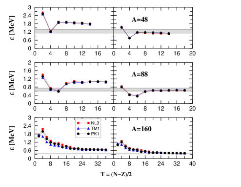
Figure 1: The mean level spacing $\varepsilon$ (left) and its counterpart (right) scaled by $m^{*}/m$ for A=48 (upper), 88 (middle) and 160 (lower) isobaric chains calculated using effective Lagrangians NL3, TM1, and PK1 as marked in the figure. The shadowed areas correspond to the empirical mean level spacing: $\varepsilon^{emp}=\dfrac{53}{A}\sim\dfrac{66}{A}~{}\text{MeV}$.

The values of $\varepsilon(A,T_{z})$ calculated for the $A$=48, 88, and 160 isobaric chains of nuclei from $T_{z}=0$ to the vicinity of the drip line are shown in the left panels of Fig. 1. The calculations have been performed for three different parameterizations of the effective Lagrangian including NL3, TM1, and PK1, respectively, which all yield very similar results. For small values of $T_{z}$, strong variations in $\varepsilon(A,T_{z})$ are seen, which are associated with shell closures. For larger values of $T_{z}$, $\varepsilon(A,T_{z})$ become less sensitive to the shell structure and its value is stabilized, $\varepsilon(A,T_{z})\approx\varepsilon(A)$. Note, that the calculated values of $\varepsilon(A)$ are much larger then the empirical estimates for the mean level spacing ${53}/{A}\leq\varepsilon^{emp}\leq{66}/{A}~{}\text{MeV}$  [Sat03] ; [Gil65] ; [Kat80] ; [Shl92] . However, after rescaling $\varepsilon^{*}(A)=(m^{*}/m)\varepsilon(A)$ by the corresponding effective masses $m^{*}/m=0.595$, $0.634$, and $0.6055$ for NL3, TM1, and PK1 respectively, the effective mean level spacing $\varepsilon^{*}(A)$ neatly falls within the empirical bounds (shaded areas), as shown in the corresponding right panels. Let us also note that with increasing $A$, i.e., from $A=48$ to $A=160$, all curves move toward the upper limit of the empirical data, reflecting the decreasing role of surface effects with increasing $A$, similar to the SHF results [Sat03] .

When comparing to the results of the SHF calculations in Ref. [Sat03] , the following two important conclusions can be made: (i) even though the values of $\varepsilon(A)$ from the RMF calculation are much larger than those from the SHF, after the effective mass scaling both models generate essentially identical results in agreement to the empirical boundaries for the mean level spacing; (ii) the results from the RMF calculations clearly confirm the general outcome of Ref. [Sat03] , that the isoscalar field generates the NSE of the form $\varepsilon T^{2}$ and that its strength is indeed governed by the mean level density rather than the kinetic energy, see also [Sat05] . Let us stress that the contribution $\varepsilon T^{2}$ can also be derived analytically using the simple iso-cranking model [Sat01x] ; [Sat03] ; [Glo04] . Note further, that the evidence and conclusions gathered from the SHF and the RMF calculations are independent of the iso-cranking model.

After obtaining the average level density $\varepsilon$, we now proceed to calculate the average effective strength $\kappa$ of the isovector potential. The effective isovector potential strength $\kappa$ is obtained from the binding energy difference between the RMF calculations with and without the isovector potential for the same nucleus. As explained later, three different types of $T$-dependence of the isovector potential are investigated:

$${E_{T}}-\tilde{E_{T}}=\dfrac{1}{2}\kappa T^{2}~{}~{}\text{and}~{}~{}\dfrac{1}{2}\kappa T(T+1)~{}~{}\text{and}~{}~{}\dfrac{1}{2}\kappa T(T+1+\varepsilon/\kappa).$$ (6)

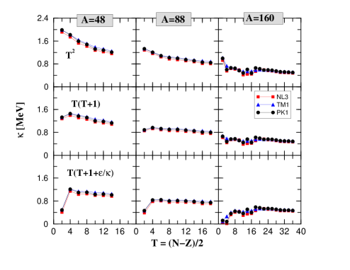
Figure 2: The average effective strength $\kappa$ of the isovector potential for A=48 (left), 88 (middle) and 160 (right) isobaric chains calculated using effective Lagrangians NL3, TM1, and PK1 as marked in the figure. Upper, middle and lower panels show the values of $\kappa$ obtained assuming $E_{\text{T}}-{\tilde{E}_{\text{T}}}=\dfrac{1}{2}\kappa T^{2}$, $\dfrac{1}{2}\kappa T(T+1)$, and $\dfrac{1}{2}\kappa T(T+1+\varepsilon/\kappa)$, respectively. See text for further details.

The resulting effective isovector potential strength $\kappa$ for A= 48, 88, and 160 isobaric chains in RMF theory are shown in Fig. 2. Similar to the SHF calculation in Ref. [Sat03] , the complicated isovector potential along an isobaric chain can be characterized by an effective isovector potential strength $\kappa(A)$. However, at variance with the SHF [Sat03] , the RMF dependence on $T$ is best reproduced by a dependence like ${E_{T}}-\tilde{E_{T}}\approx\dfrac{1}{2}\kappa T(T+1+\varepsilon/\kappa),$ rather than $T^{2}$ or $T(T+1)$. Apparently, the linear term in RMF is considerably larger than that in the SHF calculation, implying that the total NSE in RMF behaves effectively as:

$$E_{\text{sym}}\approx\dfrac{1}{2}\varepsilon T^{2}+\dfrac{1}{2}\kappa T(T+1+\varepsilon/\kappa)\approx\dfrac{1}{2}(\varepsilon+\kappa)T(T+1).$$ (7)

The important aspect to note is that in the SHF approximation the linear term originates predominantly from the Fock exchange in the isovector channel. In the RMF, which is a Hartree approximation, one would therefore expect a $\kappa T^{2}$ dependence. In contrast, the large slope of the isovector potential strength $\kappa(A,T_{z})$, fitted using either $\kappa T^{2}$ or $\kappa T(T+1)$ dependence reveals the presence of an effective linear term that is large enough to compensate the lack of the linear term in the $\varepsilon$ proportional term, see Fig. 2. Similar tendencies for the mean level spacing $\varepsilon$ and effective isovector potential strength $\kappa$ are present in all the 10 isobaric chains we calculated, including $A$=40, 48, 56, 88, 100, 120, 140, 160, 164, and 180.

At a first glance, the RMF theory is a Hartree approximation (without exchange term) and one does not expect a linear term to be present. On the other hand, the RMF as well as the SHF are two particular realizations of the density functional (DF) theory. Moreover, due to the large meson masses the relativistic forces should be close to zero range forces and both approaches are expected to be rather alike since in this limit the exchange term takes the same form as the direct term and should be effectively included within the DF. The question that arises is why the RMF is capable to generate the linear term in contrast to the SHF approach? In this context it is interesting to observe that within the RMF approach the isovector mean-potential is generated by the $\rho$-meson field. Hence, its properties are defined essentially by a single coupling constant $g_{\rho}$, see Eq. (4). In this respect the RMF seems to be more flexible than the SHF where isoscalar and isovector parts of the Skyrme local energy density functional are strongly dependent upon each other through the auxiliary Skyrme force (SF) parameters which are fitted to the data. In the process of detreminig the SF, one should therefore balance properly and very carefully the isoscalar and isovector data used in the fitting procedure. Indeed, our earlier study [Sat03] shows that the SkO [Rei99] parameterization of the SF, which has been fitted to neutron-rich nuclei, has a stronger linear term than the so called standard parameterizations but not as strong as that in RMF theory.

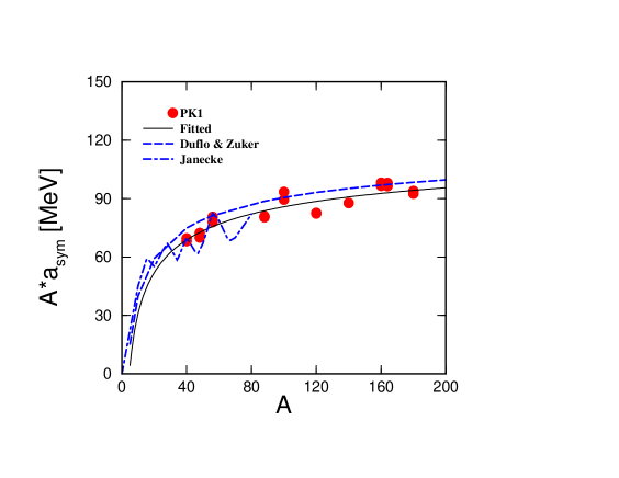
Figure 3: The nuclear symmetry energy coefficient $a_{\text{sym}}*A$ (filled circles) extracted from $E_{\text{sym}}=a_{\text{sym}}T(T+1)$ for the A=40, 48, 56, 88, 100, 120, 140, 160, 164, and 180 isobaric chains calculated using effective Lagrangian PK1. The solid line represents fit to the calculations, i.e., $A*a_{\text{sym}}=133.20-220.27/A^{1/3}$ from Eq. (9). The dashed line is from Eq. (2): $A*a_{\text{sym}}=134.4-203.6/A^{1/3}$ [Duf95] and the dot-dashed line is from Ref. [Jan65x] . For further details, see text.

We proceed further by investigating the mass dependence of the NSE. Since the total NSE in RMF theory behaves effectively like $T(T+1)$ we extract the NSE strength $a_{\text{sym}}(A)$ from the difference of the binding energies:

$$E_{\text{sym}}={E_{T}}-E_{T=0}=a_{\text{sym}}(A)T(T+1).$$ (8)

To avoid the influence of shell structure we chose two nuclei with large $T_{z}$ for each isobaric chain $A$ and calculate $a_{\text{sym}}(A)$ simply as an arithmetic mean over such a pair of nuclei. In order to compare with the empirical data of Ref. [Duf95] , we depict in Fig. 3 the product $A*a_{\text{sym}}$ as a function of $A$ for all the 10 isobaric chains calculated with the effective Lagrangian PK1. The dot-dashed line in Fig. 3 is taken from Ref. [Jan65x] revealing the shell structure of the symmetry energy coefficient and the dashed line represents a fit to experimental data given by Eq. (2) [Duf95] . The maxima at $A$=40 and $A$=56 can easily be seen in our calculation, which is in good agreement with Ref. [Jan65x] . This behavior is easy to understand since $T$=0 nuclei in the $A$=40, 56, 100 and 164 isobaric chains are double magic nuclei and hence, more bound, resulting in an increase of the symmetry energies for nuclei with $T>0$. Still, the average of the calculated symmetry energy is quite close to the dashed line, which is fitted to masses in Ref. [Duf95] .

Restricting this analysis to volume and surface terms only, a least-square fit to the calculated points (filled circles in Fig. 3) leads to a smooth curve:

$$a_{\text{sym}}^{(\text{RMF})}=\dfrac{133.20}{A}-\dfrac{220.27}{A^{4/3}}~{}\text{[MeV]},$$ (9)

shown as solid line, which is very close to the empirical values (dashed line).

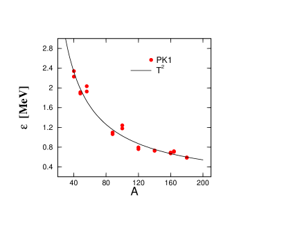
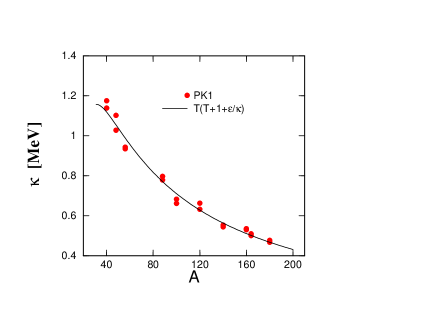
Figure 4: Volume and surface contributions to the mean level spacing $\varepsilon$ (left) and effective strength $\kappa$ (right). The fitted line is obtained from the same points as in Fig. 3, i.e., $\varepsilon=\dfrac{130.42}{A}-\dfrac{127.83}{A^{4/3}}$ and $\kappa=\dfrac{144.77}{A}-\dfrac{342.08}{A^{4/3}}$.

In a similar manner, the volume and surface contributions to the mean level spacing $\varepsilon$ and the average effective strength $\kappa$ are determined from the calculations. In the left panel of Fig. 4, the mean level spacing $\varepsilon$ (filled circles) extracted from $\tilde{E}_{T}-\tilde{E}_{T=0}=\dfrac{1}{2}\varepsilon T^{2}$ are presented together with the smooth curve obtained from least-square fit:

$$\varepsilon=\dfrac{130.42}{A}-\dfrac{127.83}{A^{4/3}}~{}\text{[MeV]}.$$ (10)

In the right panel of Fig. 4, the average effective strength $\kappa$ (filled circles) extracted from ${E}_{T}-\tilde{E}_{T}=\dfrac{1}{2}\kappa T(T+1+\varepsilon/\kappa)$ are presented together with the smooth curve obtained by least-square fit:

$$\kappa=\dfrac{144.77}{A}-\dfrac{342.08}{A^{4/3}}~{}\text{[MeV]}.$$ (11)

It should be noted that we choose the same nuclei for the fit of $\varepsilon$, $\kappa$, and $a_{\text{sym}}$ in the least-square fitting.

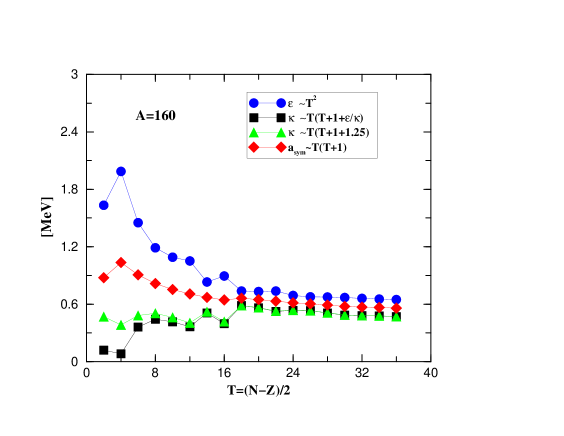
Figure 5: The mean level spacing $\varepsilon$, the average effective isovector potential strength $\kappa$ calculated assuming either $T(T+1+\varepsilon/\kappa)$ or $T(T+1+1.25)$ dependence, and the symmetry energy coefficient $a_{sym}$ for the $A=160$ isobaric chain in RMF theory with effective Lagrangian PK1. The value of 1.25 is the average for $\varepsilon/\kappa$ at $A=160$.

It was shown before that for relatively large values of $T_{z}$ both $\varepsilon(A,T_{z})\approx\varepsilon(A)$ and $\kappa(A,T_{z})\approx\kappa(A)$ along each isobaric chain. Let us now fix the value of $A$ and investigate fine effects in $\varepsilon(A,T_{z})$, $\kappa(A,T_{z})$, and $a_{sym}(A,T_{z})=\dfrac{1}{2}(\varepsilon(A,T_{z})+\kappa(A,T_{z}))$ versus $T_{z}$ in order to study the response of the isovector potential to changes in shell structure which are naturally incorporated in the mean level spacing $\varepsilon(A,T_{z})$. Therefore, we present in Fig. 5 the values of $\varepsilon(A,T_{z})$, $\kappa(A,T_{z})$, and $a_{sym}(A,T_{z})$ calculated using $T^{2}$, $T(T+1+\varepsilon/\kappa)$, and $T(T+1)$ isospin dependencies respectively, for the $A=160$ isobaric chain using the parametrization PK1 of the effective Lagrangian. To avoid the direct connection between $\kappa$ and $\varepsilon$ entering the $T(T+1+\varepsilon/\kappa)$ dependence used to extract $\kappa(A,T_{z})$ we also show values of $\kappa(A,T_{z})$ obtained assuming $T(T+1+1.25)$ dependence, where 1.25 represents the average value of $\varepsilon/\kappa$. Clearly, there are small variations in $\varepsilon(A,T_{z})$ for $T_{z}=12,14,16$ and $22$ due to the shell structure. Whilst the same variations are also obtained for $\kappa(A,T_{z})$ at the same value of $T_{z}$, the sum $a_{sym}(A,T_{z})$ is very smooth. Apparently, changes in $\varepsilon(A,T_{z})$ and $\kappa(A,T_{z})$ cancel to large extent. We also see that the variations in $\kappa(A,T_{z})$ are not due to the $\varepsilon/\kappa$ term, since similar variations are found for the $\kappa(A,T_{z})$ curve calculated using the $T(T+1+1.25)$ dependence, see also the curves for $T^{2}$ and $T(T+1)$ as shown in the right panel of Fig. 2. Apparently, the variations of $\kappa(A,T_{z})$ reflect a direct response to changes in $\varepsilon(A,T_{z})$ showing that effectively, the isovector potential and isoscalar potential become closely linked.

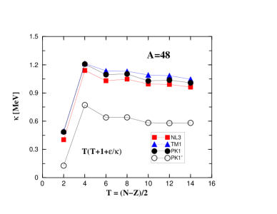
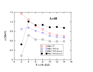
Figure 6: The comparison of the average effective strength $\kappa$ of the isovector potential for the A=48 isobaric chain between self-consistent RMF calculation (PK1) and the corresponding non self-consistent (PK1’). See the text for further explanations.

In order to understand the origin of the linear term in RMF theory, self-consistent calculations for the effective Lagrangian PK1 have been performed including the $\sigma$ and $\omega$ meson-fields only. With the nucleon densities thus obtained, the influence of the $\rho$ meson field has been extracted by switching on the isovector potential in a non-self-consistent way. The results for the $A$=48 isobaric chains are labeled as PK1’ in Fig. 6. It is interesting to note that just by switching on the isovector potential, the relation $T(T+1+\varepsilon/\kappa)$ is followed quite well, although it accounts for only $2/3$ of the total $\kappa$. We can therefore conclude that the linear term $(\varepsilon+\kappa)T$ exists in RMF whenever the isovector potential is present. The self-consistency between the isovector and isoscalar potentials roughly contributes to another $1/3$.

As shown in Fig. 3, the nuclear symmetry energy for finite nuclei calculated in RMF theory with PK1 is in good agreement with the experiment. The symmetry energy coefficient, as obtained from finite nuclei can be extrapolated to infinite nuclear matter by setting the surface term of Eq. (2) or Eq. (9) to zero. The theoretical asymptotic value obtained in this manner $a_{sym}^{\prime}\equiv A*a_{sym}/4\approx 33.6$ MeV is rather close to the empirically accepted values but considerably smaller [by $\sim$10%] than the so called infinite symmetric nuclear matter(NM) values which are equal to 37.4 MeV for NL3 [Lal97] , 36.9 MeV for TM1 [Sug95] , and 37.6 MeV for PK1 [Lon04] , respectively. The infinite NM values are obtained using the following formula [Gle97] :

$$a_{sym}^{\prime}=\frac{1}{2}\left(\frac{g_{\rho}}{m_{\rho}}\right)\rho_{0}+\frac{k_{F}^{2}}{6\sqrt{k_{F}^{2}+m^{*2}}},$$ (12)

where $\rho_{0}$ is the saturation point, $k_{F}=(3\pi^{2}\rho_{0}/2)^{1/3}$ is the Fermi momentum and $m^{*}$ is the effective mass at saturation point. One should note that the symmetry energy coefficient $a_{sym}^{\prime}$ decreases with increasing $N/Z$ ratio in infinite NM. Moreover, there are effective Lagrangians having smaller values of $a_{sym}^{\prime}$ in the infinite symmetric NM including GL-97 (32.5 MeV) [Gle97] , TW-99 (32.77 MeV) [Typ99] and DD-ME1 (33.06 MeV) [Nik02] . At present, the origin of this discrepancy is not clear to us. Certainly, it reflects the important role played by the nuclear surface in finite nuclei, where one can notice the large contribution to the surface energy coming from the isovector potential. Differences in the linear term affect the size of the surface energy coefficient obtained in the calculations. However, the volume term of the total symmetry energy coefficient is not affected much even when varying the linear term between 1 and 4.

In summary, the nuclear symmetry energy has been studied in RMF theory with effective Lagrangians NL3, TM1, and PK1. The mean level spacing $\varepsilon$, the effective isovector potential strength $\kappa$, and the nuclear symmetry energy coefficient $a_{\text{sym}}$ are calculated for the isobaric chains $A$=40, 48, 56, 88, 100, 120, 140, 160, 164, and 180 from $T=0$ to the vicinity of the drip line. It is shown that, except some strong variations at small values of $T_{z}$, the mean level spacing $\varepsilon$ is stabilized at large $T_{z}$ and lies in the region of the empirical value after being re-scaled by the effective mass. These results confirm the general formulation of the symmetry energy obtained from the simple iso-cranking model as first proposed in Ref. [Sat01x] and are in agreement with Skyrme-Hartree-Fock calculations [Sat03] ; [Sat05] .

By switching on the isovector potential due to the $\rho$ meson field, the effective isovector potential strength $\kappa$ is extracted. It is surprising to find that the RMF theory, which is a Hartree approximation at first glance, generates a large linear term corresponding at least to ${E_{T}}-\tilde{E_{T}}\approx\dfrac{1}{2}\kappa(A)T(T+1+\varepsilon/\kappa)$. This is in contrast to the SHF model, where the isovector potential has a $\dfrac{1}{2}\kappa(A)T(T+1)$ dependence. Hence, the total nuclear symmetry energy in RMF follows the $T(T+1)$ relation quite well.

The nuclear symmetry energy coefficient $a_{\text{sym}}$ as extracted from $E_{\text{sym}}=a_{\text{sym}}T(T+1)$ is in good agreement with the empirical data in Refs. [Jan65x] ; [Duf95] . The discrepancy between the calculated asymptotic value of $a_{sym}$ and the infinite symmetric nuclear matter estimate requires further systematic studies. Our work also indicates that a general formulation of the nuclear binding energy in terms of the density functional theory in fact can yield a $T(T+1)$ dependence of the symmetry energy. The question of the physical mechanism leading to the restoration of the complete linear term within RMF theory is left open.

- (1) W. Satuła and R. Wyss, Phys. Rev. Lett. 86 (2001) 4488; 87 (2001) 052504.
- (2) A. Bohr and B.R. Mottelson, Nuclear Structure, Vol. I (W.A. Benjamin, New York, 1969).
- (3) I. Talmi and R. Thieberger, Phys. Rev. 103 (1956) 718.
- (4) I. Talmi, Rev. Mod. Phys. 34 (1962) 704.
- (5) N. Zeldes, in Handbook of Nuclear Properties, Ed. by D. Poenaru and W. Greiner, Clarendon Press, Oxford, 1996, p. 13.
- (6) K. Neergård, Phys. Lett. B537 (2002) 287; Phys. Lett. B572 (2003) 159.
- (7) W. D. Myers and W. J. Swiatecki, Nucl. Phys. 81 (1966) 1.
- (8) J. Jänecke, Nucl. Phys. 73 (1965) 97; J. Jänecke et al., Nucl. Phys. A728 (2003) 23.
- (9) P. Möller et al., At. Data Nucl. Data Tables 59 (1995) 185.
- (10) J. Duflo and A. P. Zuker, Phys. Rev. C52 (1995) R23.
- (11) W. Satuła and R. Wyss, Phys. Lett. B572 (2003) 152.
- (12) S. Głowacz, W. Satuła, and R.A. Wyss, Eur. Phys. J. A19 (2004) 33.
- (13) W. Satuła and R. Wyss, Rep. Prog. Phys. 68 (2005) 131.
- (14) J. Meng and P. Ring, Phys. Rev. Lett. 77 (1996) 3963; Phys. Rev. Lett. 80 (1998) 460.
- (15) P. Ring, Prog. Part. Nucl. Phys. 37 (1996) 193.
- (16) Y. K. Gambhir, P. Ring, and A. Thimet, Ann. Phys. (N.Y.) 198 (1990) 132.
- (17) S. G. Zhou, J. Meng, and P. Ring, Phys. Rev. C68 (2003) 034323.
- (18) G.A. Lalazissis, J. König, and P. Ring, Phys. Rev. C55 (1997) R540.
- (19) Y. Sugahara, Doctor thesis, Tokyo Metropolitan University, 1995.
- (20) W.H. Long et al., Phys. Rev. C69 (2004) 034319.
- (21) S.F. Ban et al., Phys. Rev. C69 (2004) 045805.
- (22) J. Meng et al., Prog. Part. Nucl. Phys. (2005) in press; nucl-th/0508020.
- (23) A. Gilbert and A. G.W. Cameron, Can. J. Phys. 43 (1965) 1965.
- (24) S.A. Kataria and V.S. Ramamurthy, Phys. Rev. C22 (1980) 2263.
- (25) S. Shlomo, Nucl. Phys. A539 (1992) 17.
- (26) P.-G. Reinhard et al., Phys. Rev. C60 (1999) 014316.
- (27) N.K. Glendenning, Compact star, Springer-Verlag, New York, 1997.
- (28) S. Typel and H.H. Wolter, Nucl. Phys. A656 (1999) 331.
- (29) T. Niki et al., Phys. Rev. C66 (2002) 024306.