Hans Bethe: The Nuclear Many Body Problem

1 The Atomic and Nuclear Shell Models

Before the second world war, the inner workings of the nucleus were a mystery. Fermi and collaborators in Rome had bombarded nuclei by neutrons, and the result was a large number of resonance states, evidenced by sharp peaks in the cross section; i.e., in the off-coming neutrons. These peaks were the size of electron volts (eV) in width. (The characteristic energy of a single molecule flying around in the air at room temperature is the order of 1/40 of an electron volt. Thus, one electron volt is the energy of a small assemblage of these particles.) On the other hand, the difference in energy between low-lying energy levels in light and medium nuclei is the order of MeV, one million electron volts.

Now Niels Bohr’s point [1] was that if the widths of the nuclear levels (compound states) were more than a million times smaller than the typical excitation energies of nuclei, then this meant that the neutron did not just fall into the nucleus and come out again, but that it collided with the many particles in the nucleus, sharing its energy. According to the energy-time uncertainty relation, the width $\Delta E$ of such a resonance is related to the lifetime of the state by $t\simeq\hbar/\Delta E\sim\hbar/(1$ eV) . In fact, the time $t\sim\hbar/(10$ MeV) is the characteristic time for a nucleon to circle around once in the nucleus, the dimension of which is Fermis (1 Fermi = $10^{-13}$ cm). Thus, a thick “porridge” of all of the nucleons in the nucleus was formed, and only after a relatively long time would this mixture come back to the state in which one single nucleon again possessed all of the extra energy, enough for it to escape. The compound states in which the incoming energy was shared by all other particles in the porridge looked dauntingly complicated.

Now atomic physics was considered to be very different from nuclear physics, the atomic many body problem being that of explaining the makeup of atoms. Niels Bohr [2] had shown, starting with the hydrogen atom, that each negatively charged electron ran around the much smaller nucleus in one of many “stationary states.” Once in such a state, it was somehow “protected” from spiraling into the positively charged nucleus. (This “protection” was understood only later with the discovery of wave mechanics by Schrödinger and Heisenberg.) The allowed states of the hydrogen atom were obtained in the following way. The Coulomb attraction between the electron and proton provides the centripetal force, yielding

$$\frac{e^{2}}{r^{2}}=\frac{mv^{2}}{r},$$ (1)

where $-e$ is the electron charge, $+e$ is the proton charge, $m$ is the electron mass, $v$ is its velocity, and $r$ is the radius of the orbit. Niels Bohr carried out the quantization, the meaning of which will be clear later, using what is called the classical action, but a more transparent (and equivalent) way is to use the particle-wave duality picture of de Broglie (Prince L. V. de Broglie received the Nobel prize in 1929 for his discovery of the wave nature of electrons.) in which a particle with mass $m$ and velocity $v$ is assigned a wavelength

$$\lambda=\frac{h}{mv},$$ (2)

where $h$ is Planck’s constant, ubiquitous in quantum mechanics. If the wave is to be stationary, it must fit an integral number of times around the circumference of the orbit, leading to

$$n\frac{h}{mv}=2\pi r.$$ (3)

Eliminating $v$ from eqs. (1) and (3), we find the radius of the orbit to be

$$r=\frac{n^{2}\hbar^{2}}{me^{2}},\mbox{ \hskip 14.45377ptwhere \hskip 14.45377pt}\hbar=\frac{h}{2\pi}.$$ (4)

Now the kinetic energy of the electron is

$$T=\frac{1}{2}mv^{2}=\frac{e^{2}}{2r},$$ (5)

where we have used eq. (1). The potential energy is

$$V=-\frac{e^{2}}{r}=-2T,$$ (6)

which follows easily from eq. (5). Eq. (6) is known as a “virial relation,” an equation that relates the kinetic and potential energies to one another. In the case of a potential depending on $r$ as $1/r$, the kinetic energy is always equal to $-1/2$ of the potential energy. From this relation we find that the total energy is given by

$$E=T+V=-T.$$ (7)

Finally, one finds by combining eqs. (7), (5), and (4) that

$$E_{n}=-\frac{1}{2}\frac{me^{4}}{n^{2}\hbar^{2}}=-\frac{1}{n^{2}}Ry,$$ (8)

where $Ry$ is the Rydberg unit for energy

$$Ry\simeq 13.6\mbox{ electron volts.}$$ (9)

Thus, we find only a discrete set of allowed energies for an electron bound in a hydrogen atom, and we label the corresponding states by their values of $n$. Since $n=1$ for the innermost bound orbit in hydrogen, called an $s$-state for reasons we discuss later, 13.6 electron volts is the ionization energy, the energy necessary to remove the electron.

Electrons are fermions, such that only one particle can occupy a given quantum state at a time. This is called the “exclusion principle.” (Wolfgang Pauli received the Nobel prize in 1945 for the discovery of the exclusion principle, also called the “Pauli principle.”) Once an electron has been put into a state, it excludes other electrons from occupying it. However, electrons have an additional property called spin, which has the value 1/2 (in units of $\hbar$), and this spin can be quantized along an arbitrary axis to be either up or down. Thus two electrons can occupy the $1s$ state. Putting two electrons around a nucleus consisting of two neutrons and two protons makes the helium atom. Helium is the lightest element of the noble gases. (They are called “noble” because of their little chemical interaction.) Since the $1s$ shell is filled with two electrons, the helium atom is compact and does not have an empty $1s$ orbital which would like to grab a passing electron, unlike hydrogen which is very chemically active due to a vacancy in its $1s$ shell.

To go further in the periodic table we have to put electrons into the $n=2$ orbit. A new addition is that an electron in the $n=2$ state can have an orbital angular momentum of $l=0$ or $1$, corresponding to the states $2s$ and $2p$, respectively. (The spectroscopic ordering is $s\,p\,d\,f\,g\,h\,i$ for $l=0-6$, a notation that followed from the classification of atomic spectra well before the Bohr atom was formulated.) The angular momentum $l=1$ of the $2p$ state can be projected on an arbitrary axis to give components $m=1,0,$ or $-1$. So altogether, including spin, six particles can be put into the $2p$ state and two into the $2s$ state. Thus, adding eight electrons in the $2s$- and $2p$-states, the next member of the noble gases, neon, is obtained. It is particularly compact and the electrons are well bound, because both the $n=1$ and $n=2$ shells are filled.

Consider an element in which the $n=2$ shell is not filled, oxygen, which has eight electrons, two in the $n=1$ shell and six in the $n=2$ shell. Oxygen in the bloodstream or in the cellular mitochondria is always on the alert to fill in the two empty orbits. We call such a “grabbing” behavior “oxidation,” even though the grabbing of electrons from other chemical elements is done not only by oxygen. The molecules that damage living cells by stealing their electrons are called “free radicals,” and it is believed that left alone, they are a major cause of cancer and other illnesses. This is the origin of the term “oxidative stress.” We pay immense amounts of money for vitamins and other “antioxidants” in order to combat free radicals by filling in the empty states.

We need to add one further piece to the picture of the atomic shell model, the so-called $j-j$ coupling, which really gave the key success of the nuclear shell model, as we explain later. The $j$ we talk about is the total angular momentum, composed of adding the orbital angular momentum $l$ and the spin angular momentum $s$. The latter can take on projections of $+1/2$ or $-1/2$ along an arbitrary axis, so $j$ can be either $l+1/2$ or $l-1/2$. The possible projections of $j$ are $m=j,j-1,\dots,-j$. Thus, if we reconsider the $p$-shell in an atom, which has $l=1$, the projections are reclassified to be those of $j=3/2$ and $j=1/2$. The former has projections $3/2,1/2,-1/2,$ and $-3/2$, the projections differing by integers, whereas the latter has $+1/2$ and $-1/2$. Altogether there are six states, the same number that we found earlier, through projections of $m_{l}=-1,0,1$ and of $m_{s}=+1/2,-1/2$. The classification in terms of $j$ is important because there is a spin-orbit coupling; i.e., an interaction between spin and orbital motion which depends on the relative angle between the spin and orbital angular momentum. This interaction makes it more favorable for the spin to be aligned opposite to the direction of the orbital angular momentum, as in the $2p_{3/2}$ state being higher in energy than the $2p_{1/2}$ state. In this notation, the subscript refers to the total angular momentum. The filling of the shells in the $j-j$ classification scheme is the same as in the $l$ scheme in that the same number of electrons fill a shell in either scheme, the subshell labels being different, however.

The above is the atomic shell model, so called because electrons are filled in shells. The electric interaction is weak compared with the nuclear one, down by the factor of $\alpha=e^{2}/\hbar c=1/137$ from the nuclear interaction (called the strong interaction). The atomic shell model is also determined straightforwardly because the nucleus is very small (roughly 1,000 times smaller in radius than the atom), and it chiefly acts as a center about which the electrons revolve. In atoms the number of negatively charged electrons is equal to the number of positively charged protons, the neutrons being of neutral charge. In light nuclei there are equal numbers of neutrons and protons, but the number of neutrons relative to the protons grows as the mass number $A$ increases, because it is relatively costly in energy to concentrate the repulsion of the protons in the nucleus. On the whole, electric forces play only a minor role in the forces between nucleons inside the nucleus, except for determining the ratio of protons to neutrons. By the time we get to ²⁰⁸Pb with 208 nucleons, 126 neutrons and 82 protons, we come to a critical situation for the nuclear shell model, which requires the spin-orbit force, as we discuss later.

After a decade or two of nuclear “porridge,” imagine people’s surprise when the nuclear shell model was introduced in the late 1940’s [3, 4] and it worked; i.e., it explained a lot of known nuclear characteristics, especially the “magic numbers.” That is, as shells were filled in a prescribed order, those nuclei with complete shells turned out to be substantially more bound than those in which the shells were not filled. In particular, a particle added to a closed shell had an abnormally low binding energy.

What determines the center in the nuclear shell model? In the case of the atomic shell model, the much heavier and much smaller nucleus gave a center about which the electrons could be put into shells. Nuclei were known to be tightly bound. There must be a center, and most simply the center would be exactly in the middle of the charge distribution. This charge distribution can be determined by considering two nuclei that differ from one another by the exchange of a proton and a neutron. In this case the two nuclei will have different binding energies due to the extra Coulomb energy associated with the additional proton. This difference could be measured by the energy of the radioactive decay of the one nucleus into the other and estimated roughly as $Ze^{2}/R$ (where $R$ is the radius of the nucleus and $Z$ is the number of protons). This gave $R\sim 1.5A^{1/3}\times 10^{-13}$ cm, where $A$ is the mass number. (Later electron scattering experiments, acting like a very high resolution electron scattering microscope, gave the detailed shape of the charge distribution and basically replaced the 1.5 by 1.2.) Since we now have an estimate of the nuclear charge distribution, we would like to use this information to help determine the shell model potential.

Now the most common force is zero force, that is, matter staying at rest in equilibrium. The force, according to Newton’s law, is the (negative) derivative of the potential. If the potential at short distances is some constant times the square of $r$; i.e., $V=Cr^{2}$, then the force $F=-dV/dr=-2Cr$ is zero at $r=0$. Furthermore, the negative sign indicates that any movement away from $r=0$ is met by an attractive force directed back toward the center, leading to stable equilibrium. Such a potential is called a harmonic oscillator. It occurs quite commonly in nature, since most matter is more or less in equilibrium.

The energy of a particle in such a potential can be expressed classically as

$$E=\frac{p^{2}}{2M}+\frac{1}{2}M\omega^{2}r^{2},$$ (10)

where $p$ is its momentum, $M$ is its mass, and $\omega$ is a parameter that roughly describes the width of the potential well. Then one can define a length parameter $a$ through

$$\hbar\omega=\frac{\hbar^{2}}{Ma^{2}}$$ (11)

and the root mean square radius $R$ of the nucleus can be determined in terms of $A$ and $a$, $R$ being proportional to $A^{1/3}$. Using harmonic oscillator wave functions with $a$ (or $\omega$) determined so that

$$R=1.2A^{1/3}\times 10^{-13}\mbox{ cm}$$ (12)

gives a remarkably good fit to the shape of the charge distribution (in which only the protons are included) of the nucleus. The possible energy levels in such a potential are shown in Fig. 2 where we have labeled them in the same way as in the atomic shell model. Note that the distances between neighboring levels are always the same, $\hbar\omega$. We redraw the potential in Fig. 2, incorporating the $j-j$ coupling.

Figure 1: Harmonic oscillator potential with possible single-particle states.

Figure 2: Harmonic oscillator potential with possible single particle states in $j$–$j$ coupling.

Note that the spin-orbit splitting, that is, the splitting between two states with the same $l$, is somewhat smaller than the distance between shells, so that the classification of levels according to $l$ as shown in Fig. 2 gives a good zero-order description.

At first sight the harmonic oscillator potential appears unreasonable because the force drawing the particle back to the center increases as the particle moves farther away, but nucleons can certainly escape from nuclei when given enough energy. However, the last nucleon in a nucleus is typically bound by about 8 MeV, and this has the effect that its wave function drops off rapidly outside of the potential; i.e., the probability of finding it outside the potential is generally small. In fact, the harmonic oscillator potential gives remarkably good wave functions, which can only be improved upon by very detailed calculations.

In the paper of the “Bethe Bible” coauthored with R. F. Bacher [5], nuclear masses had been measured accurately enough in the vicinity of ¹⁶O so that “It may thus be said safely that the completion of the neutron-proton shell at ¹⁶O is established beyond doubt from the data about nuclear masses.” The telltale signal of the closure of a shell is that the binding energy of the next particle added to the closed shell nucleus is anomalously small. Bethe and Bacher (p. 173) give the shell model levels in the harmonic oscillator potential, the infinite square well, and the finite square well. These figures would work fine for the closed shell nuclei ¹⁶O and ⁴⁰Ca. In Fig. 2, ¹⁶O would result from filling the $1s$ and $1p$ shells, ⁴⁰Ca from filling additionally the $2s$ and $1d$ shells. However, other nuclei that were known to be tightly bound, such as ²⁰⁸Pb, could not be explained by these simple potentials.

The key to the Goeppert Mayer-Jensen success was the spin-orbit splitting, as it turned out. There were the “magic numbers,” the large binding energies of ¹⁶O, ⁴⁰Ca, and ²⁰⁸Pb. Especially lead, with 82 protons and 126 neutrons, is very tightly bound. Now it turns out (see Fig. 3) that with the strong spin-orbit splitting the $1h_{11/2}$ level for protons and the $1i_{13/2}$ level for neutrons lie in both cases well below the next highest levels. The notation here is different from that used in atomic physics. The “1” denotes that this is the first time that an $h$ ($l=5$) level would be filled in adding protons to the nucleus and for the neutron levels similarly, $i$ denoting $l=6$.

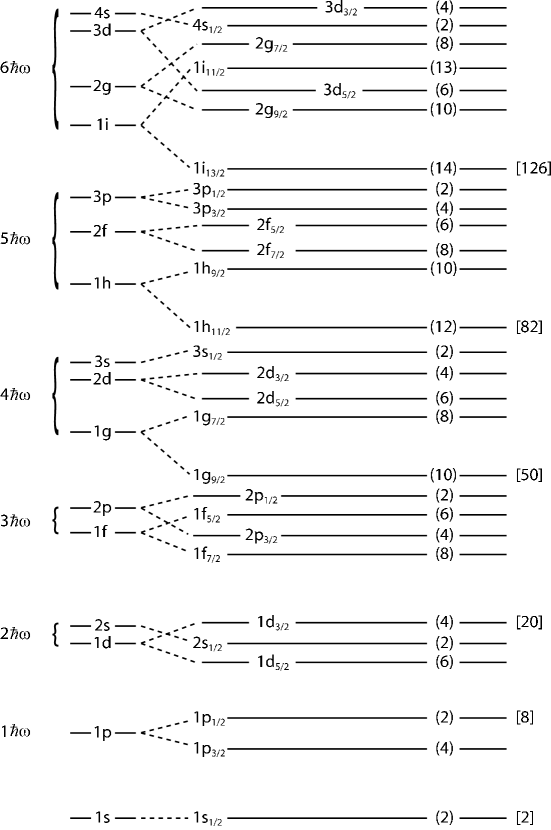
Figure 3: Sequence of single particle states in the nuclear shell model.

So how could a model in which nucleons move around in a common potential without hitting each other be reconciled with the previous “nuclear porridge” of Niels Bohr? Most of the answer came that the thorough mixture of particles in the porridge arose because the neutron was dropped into the nucleus with an energy of around 8 MeV above the ground state energy in the cases of “porridge.” At least initially the shell model was classifying ground states of systems, where they acquired no energy. The ground state was constructed by filling the lowest energy single-particle states, one by one. Later, in 1958, Landau formulated his theory of Fermi liquids, showing that as a particle (fermion) was added with energy just at the top of the highest energy occupied state (just at the top of the Fermi sea), the added particle would travel forever without exciting the other particles. In more physical terms, the mean free path (between collisions) of the particle is proportional to the inverse of the square of the difference of its momentum from that of the Fermi surface; i.e.,

$$\lambda\sim\frac{C}{(k-k_{F})^{2}},$$ (13)

where $C$ is a constant that depends on the interaction. Thus, as $k\rightarrow k_{F}$, $\lambda\rightarrow\infty$ and the particle never scatters. Here $k_{F}$, the Fermi momentum, is that of the last filled orbit.

Once the surprise had passed that one could assign a definite shell model state to each nucleon and that these particles moved rather freely, colliding relatively seldomly, the obvious question was how the self-consistent potential the particles moved in could be constructed from the interactions between the particles. The main technical problem was that these forces were very strong. Indeed, Jastrow [6] characterized the short range force between two nucleons as a vertical hard core of infinite height and radius of $0.6\times 10^{-13}$ cm, about one-third the average distance between two nucleons in nuclei. (Later, the theoretical radius of the core shrank to $0.4\times 10^{-13}$ cm.) The core was much later found to be a rough characterization of the short-range repulsion from vector meson exchange.

Now the whole postwar development of quantum electrodynamics by Feynman and Schwinger was in perturbation theory, with expansion in the small parameter $\alpha=e^{2}/\hbar c=1/137$. Of course, infinities were encountered, but since they shouldn’t be there, they were set to zero. The concept of a hard core potential of finite range, the radius a reasonable fraction of the average distance between particles, was new. Lippmann and Schwinger [7] had already developed a formalism that could deal with such an interaction. In perturbation theory; i.e., expansion of an interaction which is weak relative to other quantities, the correction to the energy resulting from the interaction is obtained by integrating the perturbing potential between the wave functions; i.e.,

$$\Delta E\simeq\int\psi_{0}^{\dagger}(x,y,z)\,V(x,y,z)\,\psi_{0}(x,y,z)\,dx\,dy\,dz.$$ (14)

Here $\psi_{0}(x,y,z)$ is the solution of the Schrödinger wave equation for the zero-order problem, that with $V(x,y,z)=0$, and $\psi_{0}^{\dagger}$ is the complex conjugate of $\psi_{0}$. The wavefunction gives the probability of finding a particle located in a small region $dx\,dy\,dz$ about the point $(x,y,z)$:

$$P(x,y,z)=\psi_{0}^{\dagger}(x,y,z)\,\psi_{0}(x,y,z)\,dx\,dy\,dz.$$ (15)

The integral in eq. (14) is carried out over the entire region in which $V(x,y,z)$ is nonzero.

Now we see the difficulty that arises if $V$ is infinite, as in the hard core potential; namely, the product of an infinite $V$ and finite $\psi$ is infinite. Eq. (14) is just the first-order correction to the energy. More generally, perturbation theory yields a systematic expansion for the energy shift in terms of integrals involving higher powers of the interaction ($V^{2},V^{3},\cdots$). As long as $\psi(x,y,z)$ is nonzero, all of these terms are infinite.

Watson [8, 9] realized that a repulsion of any strength, even an infinitely high hard core, could be handled by the formalism of Lippmann and Schwinger, which was invented in order to handle two-body scattering. Quantum mechanical scattering is described by the $T$-matrix:

$$T=V+V\frac{1}{E-H_{0}}V+V\frac{1}{E-H_{0}}V\frac{1}{E-H_{0}}V+\cdots,$$ (16)

where $V$ is the two-body potential, $E$ is the unperturbed energy, and $H_{0}$ is the unperturbed Hamiltonian, containing only the kinetic energy. This infinite number of terms could be summed to give the result

$$T=V+V\frac{1}{E-H_{0}}T.$$ (17)

One can see that this is true by rewriting eq. (16) as

$$T=V+V\frac{1}{E-H_{0}}\left(V+V\frac{1}{E-H_{0}}V+V\frac{1}{E-H_{0}}V\frac{1}{E-H_{0}}V+\cdots\right),$$ (18)

where the term in parentheses is clearly just $T$. Of course, Lippmann and Schwinger did this with the proper mathematics, but the result eq. (17) came out of this. Watson realized that the $T$-matrix made sense also for an extremely strong repulsive interaction in a system of many nucleons. An incoming particle could be scattered off each of the nucleons, one by one, and the scattering amplitudes could be added up, the struck nucleon being left in the same state as it was initially. The sum of the amplitudes could be squared to give the total amplitude for the scattering off the nucleus.

Keith Brueckner, who was a colleague of Watson’s at the University of Indiana at the time, saw the usefulness of this technique for the nuclear many-body problem. He was the first to recognize that the strong short-range interactions, such as the infinite hard core, would scatter two nucleons to momenta well above those filled in the Fermi sea. Thus, the exclusion principle would have little effect and could be treated as a relatively small correction.

Basically, for the many body problem, the $T$-matrix is called the $G$-matrix, and the latter obeys the equation

$$G=V+V\frac{Q}{e}G.$$ (19)

Whereas in the Lippmann-Schwinger formula eq. (17) the energy denominator $e$ was taken to be $E-H_{0}$, there was considerable debate about what to put in for $e$ in eq. (19). We will see later that it is most conveniently chosen to be $E-H_{0}$, as in eq. (17). In eq. (19), the operator $Q$ excludes from the intermediate states not only all of the occupied states below the Fermi momentum $k_{F}$, because of the Pauli principle, but also all states beyond a maximum momentum $k_{max}$. The states below $k_{max}$ define what is called the “model space,” which can generally be chosen at the convenience of the investigator. The basic idea is that the solution eq. (19) of $G$ is to be used as an effective interaction in the space spanned by the Fermi momentum $k_{F}$ and $k_{max}$. This effective interaction $G$ is then to be diagonalized within the model space; i.e., the problem in that space with the effective interaction $G$ is to be solved more or less exactly.

In the above discussion leading to eq. (19) we have written the nucleon-nucleon interaction as $V$. In fact, the interaction is complicated, involving various combinations of spins and angular momenta of the two interacting nucleons. In the time of Brueckner and the origin of his theory, it took a lot of time and energy just to keep these combinations straight. This large amount of bookkeeping is handled today fairly easily with electronic computers. The major problem, however, was how to handle the strong short-range repulsion, and this problem was discussed in terms of the relatively simple, what we call “central,” interaction shown in Fig. 4. In fact, the $G$ of eq. (19) is still calculated from that equation today in the most successful effective nuclear forces. The $k_{max}$ is taken to be the maximum momentum at which experiments have been analyzed, $k_{max}=2.1\mbox{ fm}^{-1}=\Lambda$, where $\Lambda$ is now interpreted as a cutoff. Since experiments of momenta higher than $\Lambda$ have not been carried out and analyzed, at least not in such a way as to bear directly on the determination of the potential, one approach is to leave them out completely. The only important change since the 1950’s is that the $V(r)$, the first term on the right hand side of eq. (19) is now rewritten in terms of a sum over momenta, by what is called a Fourier transform, and this sum is truncated at $\Lambda$, the higher momenta being discarded. The resulting effective interaction, which replaces $G$, is now called $V_{\rm low-{\it k}}$. [10, 11] We expand on this discussion at the end of this article.

The $G$-matrix of Brueckner was viewed by nuclear physicists as a complicated object. However, it is clear what the effect of a repulsion at core radius $c$ that rises to infinite height will be–it will stop the two interacting particles from going into the region of $r<c$. In non-relativistic quantum mechanics, this means that their wave function of relative motion must be zero. In other words, the wave function, whose square gives the probability of finding the particle in a given region, must be zero inside the hard core. Also, the wave function must be continuous outside, so that it must start from zero at $r=c$. Therefore, we know that the wave function must look something like that shown in Fig. 4. In any case, given the boundary condition $\psi=0$ at $r=c$, and the potential energy $V$, the wave equation can be solved for $r>c$. It is not clear at this point how $V(r)$ is to be determined and what the quantity $\psi$ is. We put off further discussion of this until Section 3, in which we develop Hans Bethe’s “Reference Spectrum.”

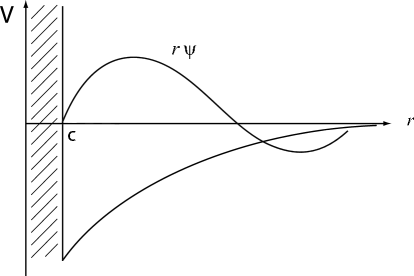
Figure 4: The wave function $\psi$ for the relative motion of two particles interacting via a potential with an infinite hard core of radius $c$ and an attractive outside potential. It is convenient to deal with $r\psi$ rather than $\psi$.

One of the most important, if not the most important, influences on Hans Bethe in his efforts, which we shall describe in the next section, to give a basis for the nuclear shell model was the work of Feshbach, Porter, and Weisskopf [12]. These authors showed that although the resonances formed by neutrons scattered by nuclei were indeed very narrow, their strength function followed the envelope of a single-particle potential; i.e., of the strength function for a single neutron in a potential $V+iW$. The strength function for the compound nucleus resonances is defined as $\bar{\Gamma}_{n}/D$, were $\Gamma_{n}$ is the width of the resonance for elastic neutron scattering (scattering without energy loss) and $D$ is the average spacing between resonances. This function gives the strength of absorption, averaged over many of the resonances. Parameters of the one-body potential are given in the caption to Fig. 5. The parameter $a$ is the surface thickness of the one-body potential.

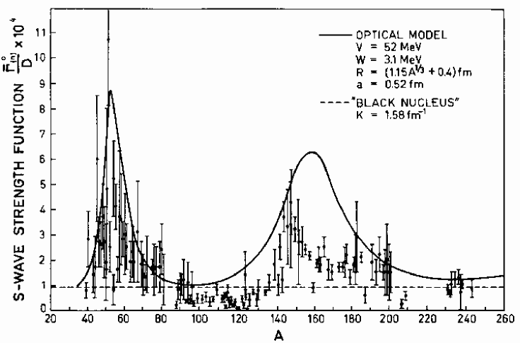
Figure 5: The $S$-wave neutron strength function as a function of mass number. This figure is taken from A. Bohr and B. R. Mottelson, Nuclear Structure, Vol. 1, p. 230, W. A. Benjamin, New York, 1969.

The peaks in the neutron strength function occur at those mass numbers where the radius of the single-particle potential is just big enough to bind another single-particle state with zero angular momentum. Although the single-particle resonance is split up into the many narrow states discussed by Bohr, a vestige of the single-particle shell model resonance still remains.

By contrast, an earlier literal interpretation of Bohr’s model was worked out by Feshbach, Peaslee, and Weisskopf in which the neutron is simply absorbed as it enters the nucleus. This curve is the dashed line called “Black Nucleus” in Fig. 5. It has no structure and clearly does not describe the variations in the averaged neutron strength function. The Feshbach, Porter, and Weisskopf paper was extremely important in showing that there was an underlying single-particle shell model structure in the individually extremely complicated neutron resonances.

In fact, the weighting function $\rho(E-E^{\prime})$ used by Feshbach, Porter, and Weisskopf to calculate the average of the scattering amplitude $S(E)$

$$\langle S(E)\rangle_{Av}=\int_{-\infty}^{\infty}\rho(E-E^{\prime})F(E^{\prime})dE^{\prime},$$ (20)

where $F(E)$ is an arbitrary (rapidly varying) function of energy $E$, was a square one that had end effects which needed to be thrown away. A much more elegant procedure was suggested by Jim Langer (see Brown [13]), which involved using the weighting function

$$\rho(E-E^{\prime})=\frac{I}{\pi}\frac{1}{(E-E^{\prime})^{2}+I^{2}}$$ (21)

With this weighting function, the average scattering amplitude was

$$\left\{\sum_{n}\frac{\Gamma(n)}{W_{n}-E}\right\}_{Av}=\sum_{n}\frac{\Gamma(n)}{W_{n}-E-iI},$$ (22)

where $W_{n}$ are the energies of the compound states with eV widths. Since the $W_{n}$ are complex numbers all lying in the lower half of the complex plane, the evaluation of the integral is carried out by contour integration, closing the contour about the upper half plane.

Now if the $I$ is chosen to be about equal to the widths of the single-neutron states in the optical model $V+iW$; i.e., of the order of $W=3.1$ MeV, then the imaginary part of this average can be obtained as

$$Im\left(\left\{\sum_{n}\frac{\Gamma(n)}{W_{n}-E}\right\}_{Av}\right)=\pi\frac{\bar{\Gamma}(n)}{D}=Im\sum_{m}\left(\frac{\Gamma_{m}}{\hat{E}_{m}-E}\right),$$ (23)

where $\Gamma_{m}$ and $\hat{E}_{m}$ are the widths and (complex) energies of the single neutron states in the complex potential $V+iW$. This shows how the averaged strength function is reproduced by the single-particle levels.

In the summer of 1958 Hans Bethe invited me (G.E.B.) to Cornell, giving me an honorarium from a fund that the AVCO Company, for which he consulted on the physics of the nose cones of rockets upon reentry into the atmosphere, had given him for that purpose. I was unsure of the convergence of the procedure by which I had obtained the above results. Hans pointed out that the width of the single-neutron state $Im(\Gamma_{m})$ would be substantially larger than the widths of the two-particle, one-hole states that the single-particle state would decay into, because in the latter the energy would be divided into the three excitations, two particles and one hole, and the widths went quadratically with available energy as can be obtained from eq. (13); ergo the two-particle, one-hole widths would be down by a factor of $\sim 3/9=1/3$ from the single-particle width, but nonetheless would acquire the same imaginary part $I$, which is the order of the single particle width in the averaging. Thus, my procedure would be convergent. So I wrote my Reviews of Modern Physics article [13], which I believe was quite elegant, beginning with Jim Langer’s idea about averaging and ending with Hans Bethe’s argument about convergence. I saw then clearly the advantage of having good collaborators, but had to wait two more decades until I could lure Hans back into astrophysics where we would really collaborate tightly.

2 Hans Bethe in Cambridge, England

We pick up Hans Bethe at the time of his sabbatical in Cambridge, England. The family, wife Rose, and children, Monica and Henry, were with him.

There was little doubt that Keith Brueckner had a promising approach to attack the nuclear many body problem; i.e., to describe the interactions between nucleons in such a way that they could be collected into a general self-consistent potential. That potential would have its conceptual basis in the Hartree-Fock potential and would turn out to be the shell model potential, Hans realized.

Douglas Hartree was professor at the University of Manchester when he invented the self-consistent Hartree fields for atoms in 1928. He put $Z$ electrons into wave functions around a nucleus of $Z$ protons, $A-Z$ neutrons, the latter having no effect because they had no charge. The heavy compact nucleus was taken to be a point charge at the origin of the coordinate system, because the nucleon mass is nearly 2000 times greater than the electron and the size of the nucleus is about 1000 times smaller in radius than that of the atom. The nuclear charge $Ze$ is, of course, screened by the electron charge as electrons gather about it. The two innermost electrons are very accurately in $1s$ orbits (called $K$-electrons in the historical nomenclature). Thus, the other $Z-2$ electrons see a screened charge of ($Z-2$)$e$, and so it could go, but Hartree used instead the so-called Thomas-Fermi method to get a beginning approximation to the screened electric field.

Given this screened field as a function of distance $r$, measured from the nucleus located at $r=0$, Hartree then sat down with his mechanical computer punching buttons as his Monromatic or similar machine rolled back and forth, the latter as he hit a return key. (G.E.B.–These machines tore at my eyes, giving me headaches, so I returned to analytical work in my thesis in 1950. Hans used a slide rule, whipping back and forth faster than the Monromatic could travel, achieving three-figure accuracy.) When Hartree had completed the solution of the Schrödinger equation for each of the original $Z$ electrons, he took its wave function and squared it. This gave him the probability, $\rho_{i}(x_{i},y_{i},z_{i})$, of finding electron $i$ at the position given by the coordinates $x_{i},y_{i},z_{i}$. Then, summing over $i$, with $x_{i}=x$, $y_{i}=y$, and $z_{i}=z$

$$\sum_{i}\rho_{i}(x,y,z)=\rho_{e}^{(1)}(x,y,z)$$ (24)

gave him the total electron density at position ($x$, $y$, $z$). Then he began over again with a new potential

$$V^{(1)}=\frac{Ze}{r}-e\rho_{e}^{(1)}(x,y,z),$$ (25)

where superscript (1) denotes that this is a first approximation to the self-consistent potential. To reach approximation (2) he repeated the process, calculating the $Z$ electronic wave functions by solving the Schrödinger equation with the potential $V^{(1)}$. This gave him the next Hartree potential $V^{(2)}$. He kept going until the potential no longer changed upon iteration; i.e., until $V^{(n+1)}\simeq V^{(n)}$, the $\simeq$ meaning that they were approximately equal, to the accuracy Hartree desired. Such a potential is called “self-consistent” because it yields an electron density that reproduces the same potential.

Of course, this was a tedious job, taking months for each atom (now only seconds with electronic computers). Some of the papers are coauthored, D. R. Hartree and W. Hartree. The latter Hartree was his father, who wanted to continue working after he retired from employment in a bank. In one case, Hartree made a mistake in transforming his units $Z$ and $e$ to more convenient dimensionless units, and he performed calculations with these slightly incorrect units for some months. Nowadays, young investigators might nonetheless try to publish the results as referring to a fractional $Z$, hoping that fractionally charged particles would attach themselves to nuclei, but Hartree threw the papers in the wastebasket and started over.

Douglas Hartree was professor in Cambridge in 1955 when Hans Bethe went there to spend his sabbatical. The Hartree method was improved upon by the Russian professor Fock, who added the so-called exchange interaction which enforced the Pauli exclusion principle, guaranteeing that two electrons could not occupy the same state. We shall simply enforce this principle by hand in the following discussion, our purpose here being to explain what “self-consistent” means in the many-body context. Physicists generally believe self-consistency to be a good attribute of a theory, but Hartree did not have to base his work only on beliefs. Given his wave functions, a myriad of transitions between atomic levels could be calculated, and their energies and probabilities could be compared with experiment. Douglas Hartree became a professor at Cambridge. This indicates the regard in which his work was held.

The shell model for electrons reached success in the Hartree-Fock self-consistent field approach. This was very much in Hans Bethe’s mind, when he set out to formulate Brueckner theory so that he could obtain a self-consistent potential for nuclear physics. He begins his 1956 paper [14] on the “Nuclear Many-Body Problem” with “Nearly everybody in nuclear physics has marveled at the success of the shell model. We shall use the expression ‘shell model’ in its most general sense, namely as a scheme in which each nucleon is given its individual quantum state, and the nucleus as a whole is described by a ‘configuration,’ i.e., by a set of quantum numbers for the individual nucleons.”

He goes on to note that even though Niels Bohr had shown that low-energy neutrons disappear into a “porridge” for a very long time before re-emerging (although Hans was not influenced by Bohr’s paper, because he hadn’t read it; this may have given him an advantage as we shall see), Feshbach, Porter, and Weisskopf had shown that the envelope of these states followed that of the single particle state calculated in the nuclear shell model, as we noted in the last section.

Bethe confirms “while the success of the model [in nuclear physics] has thus been beyond question for many years, a theoretical basis for it has been lacking. Indeed, it is well established that the forces between two nucleons are of short range, and of very great strength, and possess exchange character and probably repulsive cores. It has been very difficult to see how such forces could lead to any over-all potential and thus to well-defined states for the individual nucleons.”

He goes on to say that Brueckner has developed a powerful mathematical method for calculating the nuclear energy levels using a self-consistent field method, even though the forces are of short range.

“In spite of its apparent great accomplishments, the theory of Brueckner et al. has not been readily accepted by nuclear physicists. This is in large measure the result of the very formal nature of the central proof of the theory. In addition, the definitions of the various concepts used in the theory are not always clear. Two important concepts in the theory are the wave functions of the individual particles, and the potential $V_{c}$ ‘diagonal’ in these states. The paper by Brueckner and Levinson [15] defines rather clearly how the potential is to be obtained from the wave functions, but not how the wave functions can be constructed from the potential $V_{c}$. Apparently, BL assume tacitly that the nucleon wave functions are plane waves, but in this case, the method is only applicable to an infinite nucleus. For a finite nucleus, no prescription is given for obtaining the wave functions.”

Hans then goes on to define his objective, which will turn out to develop into his main activity for the next decade or more: “It is the purpose of the present paper to show that the theory of Brueckner gives indeed the foundation of the shell model.”

Hans was rightly very complimentary to Brueckner, who had “tamed” the extremely strong short-ranged interactions between two nucleons, often taken to be infinite in repulsion at short distances at the time. On the other hand, Brueckner’s immense flurry of activity, changing and improving on previous papers, made it difficult to follow his work. Also, the Watson input scattering theory seemed to give endless products of scattering operators, each appearing to be ugly mathematically (“Taming” thus was the great accomplishment of Watson and Brueckner). And in the end, the real goal was to provide a quantitative basis for the nuclear shell model, based on the nucleon-nucleon interaction, which was being reconstructed from nucleon-nucleon scattering experiments at the time.

The master at organization and communication took over, as he had done in formulating the “Bethe Bible” during the 1930’s.

One can read from the Hans Bethe archives at Cornell that Hans first made 100 pages of calculations reproducing the many results of Brueckner and collaborators, before he began numbering his own pages as he worked out the nuclear many body problem. He carried out the calculations chiefly analytically, often using mathematical functions, especially spherical Bessel functions, which he had learned to use while with Sommerfeld. When necessary, he got out his slide rule to make numerical calculations.

During his sabbatical year, Hans gave lectures in Cambridge on the nuclear many body problem. Two visiting American graduate students asked most of the questions, the British students being reticent and rather shy. But Professor Neville Mott asked Hans to take over the direction of two graduate students, Jeffrey Goldstone and David Thouless, the former now professor at M.I.T. and the latter professor at the University of Washington in Seattle. We shall return to them later.

As noted earlier, the nuclear shell model has to find its own center “self-consistently.” Since it is spherically symmetrical, this normally causes no problem. Simplest is to assume the answer: begin with a deep square well or harmonic oscillator potential and fill it with single particle eigenstates as a zero-order approximation as Bethe and Bacher [5] did in their 1936 paper of the Bethe Bible. Indeed, now that the sizes and shapes of nuclei have been measured by high resolution electron microscopes (high energy electron scattering), one can reconstruct these one-particle potential wells so that filling them with particles reproduces these sizes and shapes. The wave functions in such wells are often used as assumed solutions to the self-consistent potential that would be obtained by solving the nuclear many-body problem.

We’d like to give the flavor of the work at the stage of the Brueckner theory, although the work using the “Reference-Spectrum” by Bethe, Brandow, and Petschek [17], which we will discuss later, will be much more convenient for understanding the nuclear shell model. The question we consider is the magnitude of the three-body cluster terms; i.e., the contribution to the energy from the interaction of three particles. (Even though the elementary interaction may be only a two-particle one, an effective three-body interaction arises inside the nucleus, as we shall discuss.) One particular three-body cluster will be shown in Fig. 10. The three-body term, called a three-body cluster in the Brueckner expansion, is

$$\Delta E_{3}=\sum_{ijk}\left\langle\Phi_{0}\left|I_{ij}\frac{Q}{e_{ji}}I_{jk}\frac{Q}{e_{ki}}I_{ki}\right|\Phi\right\rangle.$$ (26)

Here the three nucleons $i$, $j$, and $k$ are successively excited. There are, of course, higher order terms in which more nucleons are successively excited and de-excited. In this cluster term, working from right to left, first there is an interaction $I_{ki}$ between particles $i$ and $k$. In fact, this pair of particles is allowed to interact any number of times, the number being summed into the $G$-matrix $G_{ik}$. We shall discuss the $G$-matrix in great detail later. Then the operator $Q$ excludes all intermediate states that are occupied by other particles–the particle $k$ can only go into an unoccupied state before interacting with particle $j$. The denominator $e_{ki}$ is the difference in energy between the specific state $k$ that particle $i$ goes to and the state that it came from. The particle $k$ can make virtual transitions, transitions that don’t conserve energy, because of the Heisenberg uncertainty principle

$$\Delta E\Delta t\gtrsim\hbar.$$ (27)

Thus, if $\Delta E\Delta t>\hbar$, then the particle can stay in a given state only a time

$$t=\hbar/e_{ki}$$ (28)

so the larger the $e_{ki}$ the shorter the time that the particle in a given state can contribute to the energy $\Delta E_{3}$. (Of course, the derivation of $\Delta E_{3}$ is carried out in the standard operations of quantum mechanics. We bring in the uncertainty principle only to give some qualitative understanding of the result.) Once particle $k$ has interacted with particle $j$, particle $j$ goes on to interact with the original particle $i$, since the nucleus must be left in the same ground state $\Phi_{0}$ that it began in, if the three-body cluster is to contribute to its energy.

Bethe’s calculation gave

$$\Delta E_{3}/A=-0.66\mbox{ MeV}$$ (29)

corrected a bit later in the paper to $-0.12$ MeV once only the fraction of spin-charge states allowed by selection rules are included. This is to be compared with Brueckner’s $-0.007$ MeV. Of course, these are considerably different, but this is not the main point. The main point is that both estimates are small compared with the empirical nuclear binding energy.

Thus, it was clear that the binding energy came almost completely from the two-body term $G_{ik}$, and that the future effort should go into evaluating this quantity, which satisfies the equation

$$G=V+V\frac{Q}{e}G.$$ (30)

(We will have different $G$’s for the different charge-spin states.)

Although written in a deceptively simple way, this equation is ugly, involving operators in both the coordinates $x$, $y$, $z$, and their derivatives. However, $G$ can be expressed as a two-body operator (see Section 3). It does not involve a sum over the other particles in the nucleus, so the interactions can be evaluated one pair at a time.

Thus, the first paper of Bethe on the nuclear many body problem collected the work of Brueckner and collaborators into an orderly formalism in which the evaluation of the two-body operators $G$ would form the basis for calculating the shell model potential $V(r)$. Bethe went on with Jeffrey Goldstone to investigate the evaluation of $G$ for the extreme infinite-height hard core potential, and he gave David Thouless the problem that, given the empirically known shell model potential $V_{SM}(r)$, what properties of $G$ would reproduce it.

As we noted in the last section, an infinite sum over the two-body interaction is needed in order to completely exclude the two nucleon wave functions from the region inside the (vertical) hard core. As noted earlier, Jastrow [6] had proposed a vertical hard core, rising to $\infty$, initially of radius $R_{c}=0.6\times 10^{-13}$ cm. This is about 1/3 of the distance between nucleons, so that removing this amount of space from their possible occupancy obviously increases their energy. (From the Heisenberg Principle $\Delta p_{x}\Delta x\gtrsim\hbar$, which is commonly used to show that if the particles are confined to a smaller amount of volume, the $\Delta x$ is decreased, so the $\Delta p_{x}$, which is of the same general size as $p_{x}$, is increased.) Thus, as particles were pushed closer together with increasing density, their energy would be greater. Therefore, the repulsive core was thought to be a great help in saturating matter made up of nucleons. One of the authors (G.E.B.) heard a seminar by Jastrow at Yale in 1949, and Gregory Breit, who was the leading theorist there, thought well of the idea. Indeed, we shall see later that Breit played an important role in providing a physical mechanism for the hard core as we shall discuss in the next section. This mechanism actually removed the “sharp edges” which gave the vertical hard core relatively extreme properties. So we shall see later that the central hard core in the interaction between two nucleons isn’t vertical, rather it’s of the form

$$\mbox{Hard Core }=\frac{C}{r}\mbox{ exp}\left(-\frac{m_{\omega}r}{\hbar c}\right),$$ (31)

where $\hbar/m_{\omega}c$ is $0.25\times 10^{-13}$ cm, and $m_{\omega}$ is the mass of the $\omega$-meson. The constant $C$ is large compared with unity

$$C\gg 1$$ (32)

so that the height of the core is many times the Fermi energy; i.e., the energy measured from the bottom of the shell model potential well up to the last filled level. Thus, although extreme, treating the hard core potential gives a caricature problem. Furthermore, solving this problem in “Effect of a repulsive core in the theory of complex nuclei,” by H. A. Bethe and J. Goldstone [16] gave an excellent training to Jeffrey Goldstone, who went on to even greater accomplishments. (The Goldstone boson is named after him; it is perhaps the most essential particle in QCD.)

We will find in the next section that the Moszkowski-Scott separation method is a more convenient way to treat the hard core. And this method is more practical because it includes the external attractive potential at the same time. However, even though the wave function of relative motion of the two interacting particles cannot penetrate the hard core, it nonetheless has an effect on their wave function in the external region. This effect is conveniently included by changing the reduced mass of the interacting nucleons from $M^{\star}$ to $0.85M^{\star}$ for a hard core radius $r_{c}=0.5\times 10^{-13}$ cm, and to $\sim 0.9M^{\star}$ for the presently accepted $r_{c}=0.4\times 10^{-13}$ cm.

3 The Reference-Spectrum Method for Nuclear Matter

We take the authors’ prerogative to jump in history to 1963, to the paper of H. A. Bethe, B. H. Brandow, and A. G. Petschek [17] with the title that of this section, because this work gives a convenient way of discussing essentially all of the physical effects found by Bethe and collaborators, and also the paper by S. A. Moszkowski and B. L. Scott [18] the latter paper being very important for a simple understanding of the $G$-matrix. In any case, the reference-spectrum included in a straightforward way all of the many-body effects experienced by the two interacting particles in Brueckner theory, and enabled the resulting $G$-matrix to be written as a function of $r$ alone, although separate functions $G_{l}(r)$ had to be obtained for each angular momentum $l$.

Let us prepare the ground for the reference-spectrum, including also the Moszkowski-Scott method, by a qualitative discussion of the physics involved in the nucleon-nucleon interaction inside the nucleus, say at some reasonable fraction of nuclear matter density. We introduce the latter so we can talk about plane waves locally, as an approximation. For simplicity we take the short-range repulsion to come from a hard core, of radius $0.4\times 10^{-13}$ cm.

(i) In the region just outside the hard core, the influence of neighboring nucleons on the two interacting ones is negligible, because the latter have been kicked up to high momentum states by the strong hard-core interaction and that of the attractive potential, which is substantially stronger than the local Fermi energy of the nucleons around the two interacting ones. Thus, one can begin integrating out the Schrödinger equation for $r\psi(r)$, starting from $r\psi(r)=0$ at $r=r_{c}$. The particles cannot penetrate the infinitely repulsive hard core (see Fig. 6), so their wave function begins from zero there. In fact, the Schrödinger equation is one of relative motion; i.e., a one-body equation in which the mass is the reduced mass of the two particles, $M_{N}/2$ for equal mass nucleons. As found by Bethe and Goldstone, the $M_{N}$ will be changed to $M_{N}^{\star}$ in the many-body medium, but the mass is modified not only by the hard core but also by the attractive part of the two-body potential, which we have not yet discussed.

(ii) We consider the spin-zero $S=0$ and spin-one $S=1$ states; i.e., for angular momentum $l=0$. These are the most important states. We compare the spin-one state in the presence of the potential with the unperturbed one; i.e., the one in the absence of a potential.

Before proceeding further with Hans Bethe’s work, let us characterize the nice idea of Moszkowski and Scott in the most simple possible way.

Choose the separation point $d$ such that

$$\left.\frac{d\psi(r)/dr}{\psi(r)}\right|_{r=d}=\left.\frac{d\phi(r)/dr}{\phi(r)}\right|_{r=d}$$ (33)

Technically, this is called the equality of logarithmic derivatives. As shown in Fig. 6, such a point will be there, because $r\psi$, although it starts from zero at $r=c$, has a greater curvature than $r\phi$. Now if only the potential inside of $d$ were present; i.e., if $V(r)=0$ for $r>d$, then eq. (33) in quantum mechanics is just the condition that the inner potential would produce zero scattering, the inner attractive potential for $r<d$ just canceling the repulsion from the hard core. Of course, if eq. (33) is true for a particular $k$, say $k\lesssim k_{F}$, then it will not be exactly true for other $k$’s. On the other hand, since the momenta in the short-distance wave function are high compared with $k_{F}$, due to the infinite hard core, and the very deep interior part of the attractive potential that is needed to compensate for it, eq. (33) is nearly satisfied for all momenta up to $k_{F}$ if the equality is true for one of the momenta.

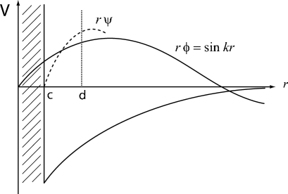
Figure 6: The unperturbed $S$-wave function $r\phi=\mbox{sin }kr$ and the wave function $r\psi$ obtained by integrating the Schrödinger equation in the presence of the potential out from $r=c$.

The philosophy here is very much as in Bethe’s work “Theory of the Effective Range in Nuclear Scattering” [19]. This work is based on the fact that the inner potential (we could define it as $V(r)$ for $r<d$) is deep in comparison with the energy that the nucleon comes in with, so that the scattering depends only weakly on this (asymptotic) energy. In fact, for a potential which is Yukawa in nature

$$V=\infty,\mbox{ for }r<c=0.4\times 10^{-13}\mbox{ cm}$$ (34)

$$V=-V_{0}e^{-(r-c)/R}\mbox{ for }r>c,$$ (35)

then $V_{0}=380$ MeV and $R=0.45\times 10^{-13}$ cm in order to fit the low energy neutron-proton scattering [20]. The value of $380$ MeV is large compared with the Fermi energy of $\sim 40$ MeV. In the collision of two nucleons, the equality of logarithmic derivatives, eq. (33), would mean that the inner part of the potential interaction up to $d$, which we call $V_{s}$, would give zero scattering. All the scattering would be given by the long-range part which we call $V_{l}$.

(iii) Now we know that the wave function $\psi(r)$ must “heal” to $\phi(r)$ as $r\rightarrow\infty$, because of the Pauli principle. There is no other place for the particle to go, because for $k$ below $k_{F}$ all other states are occupied. Delightfully simple is to approximate the healing by taking $\psi$ equal to $\phi$ for $r>d$.

The conclusion of the above is that

$$G(r)\simeq G_{s}+v_{l}(r)+v_{l}\frac{Q}{e}v_{l}+\cdots,$$ (36)

where

$$v_{l}=V(r)\mbox{ for }r\gtrsim d.$$ (37)

We shall discuss $G_{s}$, the $G$-matrix which would come from the short-range part of the potential for $r<d$ later. It will turn out to be small.

Now we have swept a large number of problems under the rug, and we don’t apologize for it because eq. (36) gives a remarkably accurate answer. However, first we note that there must be substantial attraction in the channel considered in order for the short-range repulsion to be canceled. So the separation method won’t work for cases where there is little attraction. Secondly, a number of many-body effects have been discarded, and these had to be considered by Bethe, Brandow, and Petschek, one by one.

We do not want to fight old battles over again, but simply note that Bethe, Brandow, and Petschek found that they could take into account the many-body effects including the Pauli principle by choosing a single-particle spectrum, which is approximated by

$$\epsilon_{m}=\frac{k_{m}^{2}}{2m^{\star}_{RS}}+A.$$ (38)

The parameters $m^{\star}_{RS}$ and $A$ were arrived at by a self-consistency process. The hole energies; i.e., the energies of the initially bound particles, can be treated fairly roughly since they are much smaller than the energies of the particles which have quite high momenta (see Fig. 7). Given an input $m^{\star}_{RS}$ and $A$, the same $m^{\star}_{RS}$ and $A$ must emerge from the calculation. Thus, the many-body effects can be included by changing the single-particle energy through the coefficient of the kinetic energy and by adding the constant $A$. In this way the many-body problem is reduced to the Lippmann-Schwinger two-body problem with changed parameters, $m\rightarrow m^{\star}_{RS}$ and the addition of $A$. As shown in Fig. 7, the effect is to introduce a gap $\Delta_{RS}$ between particle and hole states.

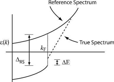
Figure 7: Energy spectrum in the Brueckner theory (inclusive of self-energy insertion). The true spectrum has a small gap $\Delta E$ at $k_{F}$ and is known, from the arguments of Bethe et al., to join the reference-spectrum at $k\approx 3$ fm^-1. The dotted line is an interpolation between these two points.

A small gap, shown as $\Delta E$, occurs naturally between particle and hole states, resulting from the unsymmetrical way they are treated in Brueckner theory, the particle-particle scattering being summed to all orders. The main part of the reference-spectrum gap $\Delta_{RS}$ is introduced so as to numerically reproduce the effects of the Pauli Principle. That this can be done is not surprising, since the effect of either is to make the wave function heal more rapidly to the noninteracting one.

Before we move onwards from the reference-spectrum, we want to show the main origin of the reduction of $m$ to $m^{\star}_{RS}\sim 0.8m$. Such a reduction obviously increases the energies of the particles in intermediate states $\epsilon(k)$ which depends inversely on $m^{\star}_{RS}$. A lowering of $m^{\star}$ from $m$ was already found in the Bethe-Goldstone solution of the scattering from a hard core alone with $m^{\star}=0.85m$ for a hard core radius of $r_{c}=0.5\times 10^{-13}$ cm and somewhat less for $r_{c}=0.4\times 10^{-13}$ cm, a more reasonable value. The $m^{\star}_{RS}$ are not much smaller than this.

Now we have to introduce the concept of off-energy-shell self energies. Let’s begin by defining the on-shell self-energy which is just the energy of a particle in the shell model or optical model potential. It would be given by the process shown in Fig. 8.

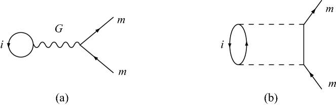
Figure 8: (a) The on-shell self energy involves the interaction of a particle in state $m$ with the filled states in the Fermi sea $i$. The wiggly line $G$ implies a sum over all orders in a ladder of $V$, the second-order term in dashed lines being shown in (b). Together with the kinetic energy, this gives the self energy.

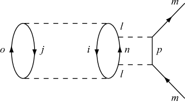
Figure 9: Second-order contribution to the self energy of a particle in state $m$ when present in a process contributing to the ground-state energy. The states $l,m,n,o,p$ refer to particles and $i,j$ to holes.

The on-shell $U(k_{m})$ should just give the potential energy of a nucleon of momentum $k$ in the optical model potential $U+iW$ used by Feshbach, Porter, and Weisskopf, so $U(k_{m})+k_{m}^{2}/2m$ gives the single-particle energy.

However, the energies $U(k_{m})$ to be used in Brueckner theory are not on-shell energies. This is because another particle must be excited when the one being considered is excited, as shown in Fig. 9. Thus, considering the second order in $V$ interaction between the particle being considered and those in the nucleus one has

$$\tilde{\epsilon}^{(2)}_{p}=-\sum_{p,n>k_{F};i<k_{F}}\frac{\left|\langle np\left|V\right|lm\rangle\right|^{2}}{\epsilon_{n}+\epsilon_{p}+\epsilon_{o}-\epsilon_{j}-\epsilon_{i}-\epsilon_{m}}$$ (39)

i.e., although the particle in state $o$ and the hole in state $j$ do not enter actively into the self energy of $p$, one must include their energies in the energy denominator. Defining

$$\tilde{\epsilon}=\epsilon_{n}+\epsilon_{p}+\epsilon_{o}-\epsilon_{j}-\epsilon_{i}-\epsilon_{m},$$ (40)

$$e=\epsilon_{n}+\epsilon_{p}-\epsilon_{i}-\epsilon_{m}$$ (41)

one sees that the additional energy in the denominator in eq. (39) is

$$\Delta e=\tilde{\epsilon}-\epsilon=\epsilon_{o}-\epsilon_{j}.$$ (42)

This $\Delta e$ represents the energy that must be “borrowed” in order to excite the particle from state $j$ to $o$, even though this particle does not directly participate in the interaction on state $p$ which gives its self energy. The point is that because $j$ must also be excited, as well as the particles on the right in the diagram of Fig. 9, the total $\tilde{e}$ is that much greater than the $e$ necessary to give the on-shell energy. Thus, the time that this interaction can go on for is decreased, since, from the uncertainty principle the time that energy can be borrowed for goes as $\Delta t=\hbar/\Delta E$. As noted earlier, the wave function $\psi(r)$ lies outside the hard core, so that integrals over the $G$-matrix are only over the attractive interaction. These are cut down by the additional energy denominator that comes in by the interaction being off shell. In the higher momentum region this can cut the self energy down by 15–20 MeV. We shall see later that when this is handled properly, only $\sim 1/3$ of this survives.

The strategy that T. T. S. Kuo and one of the authors (G.E.B.) have employed over many years, beginning with Kuo and Brown [21] to calculate the $G$-matrix in nuclei has been to use the separation method for the $G$ in the $l=0$ states ($S$-states), which have a large enough attraction so that a separation distance $d$ can be defined, but to use the Bethe, Brandow, and Petschek reference-spectrum in angular momentum states which do not have this strong attraction.

The reference-spectrum was as far as one could get using only two-body clusters; i.e., summing up the two-body interaction. In order to make further progress, three and four-body clusters had to be considered; i.e., processes in which one pair of the initially interacting particles was left excited while another pair interacted, and only then returned to its initial state as in the calculations of the lowest order three-body cluster $\Delta E_{3}$, eq. (26).

Hans Bethe investigated the four-body cluster in Ref. [22], following work on three-nucleon clusters in nuclear matter by his post-doc R. (Dougy) Rajaraman in Ref. [23], a paper just following the Bethe, Brandow, and Petschek reference-spectrum paper. Rajaraman suggested on the basis of including the other three-body clusters than that shown in Fig. 8, that the off-shell effect should be decreased by a factor of $\sim 1/2$. (We shall see from Bethe’s work below that it should actually be more like $\sim 1/3$.) Bethe first made a fairly rough calculation of the four-body clusters, but good enough to show when summed to all orders in $G$, it was tremendous, giving

$$\Delta E_{4}\simeq-35\mbox{ MeV/particle}$$ (43)

to the binding energy.

Visiting CERN in the summer of 1964, Bethe learned of Fadeev’s solution of the three-body problem [24]. Hans found that he could write expressions for the three-body problem, using the $G$-matrix as effective interaction; e.g.,

$$T\Phi=V\psi,$$ (44)

with $T$ satisfying the equation

$$T=V+V\frac{1}{e}T$$ (45)

where $e$ now represents the energy denominator of all three particles. The $T$ can be split into

$$T=T^{(1)}+T^{(2)}+T^{(3)}$$ (46)

but now one defines

$$T^{(1)}=V_{23}+V_{23}\frac{1}{e}T,$$ (47)

etc. In other words, $T^{(1)}$ denotes that part of $T$ in which particle “1” did not take part in the last interaction. The ground state energy is given by

$$E_{0}=\langle\Phi\left|T\right|\Phi\rangle,$$ (48)

where $\Phi$ is the unperturbed (free-particle) wave function. In short, one could use the Brueckner $G$-matrices as effective interactions in the Fadeev formalism, which then summed the three-body cluster terms to all orders in the solution of these equations.

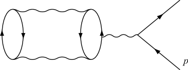
Figure 10: The contribution of the three-body cluster to the off-shell self energy of a particle in state $p$. The wiggly line here represents the $G$-matrix. One particular contribution to this is shown in Fig. 9.

Hans came to Copenhagen in late summer of 1964, with the intention of solving the Fadeev equations for the three-body system using the reference-spectrum approximation eq. (38) for the effective two-body interaction. David Thouless, Hans’ Ph.D. student in Cambridge, was visiting Nordita (Nordic Institute of Theoretical Atomic Physics) at that time. I (G.E.B.) got David together with Hans the morning after Hans arrived. Hans wrote down the three coupled equations on the blackboard and began to solve them by some methods Dougy Rajaraman had used for summing four-body clusters. David took a look at the three coupled equations with Hans’ $G$-matrix reference-spectrum approximation for the two-body interaction and said “These are just three coupled linear equations. Why don’t you solve them analytically?” By late morning Hans had the solution, given in his 1965 paper. The result, which can be read from this paper, is that the off-shell correction to the three-body cluster of Fig. 10 should be cut down by a factor of $1/3$. Hans’ simple conclusion was “when three nucleons are close together, an elementary treatment would give us three repulsive pair interactions. In reality, we cannot do more than exclude the wave function from the repulsive region, hence we get only one core interaction rather than 3.”

In the summer of 1967, I (G.E.B.) gave the summary talk of the International Nuclear Physics meeting held in Tokyo, Japan. This talk is in the proceedings. I designed my comments as letters to the speakers, as did Herzog in Saul Bellow’s novel by that name.

“Dear Professor Bethe,

First of all, your note is too short to be intelligible. But by valiant efforts, and a high degree of optimism in putting together corrections of the right sign, you manage to get within 3 MeV/particle of the binding energy of nuclear-matter. It is nice that there are still some discrepancies, because we must have some occupation for theorists, in calculating three-body forces and other effects.

Most significantly, you confirm that it is a good approximation to use plane-wave intermediate states in calculation of the G-matrix. This simplifies life in finite nuclei immensely.

I cannot agree with you that there is no difference between hard- and soft-core potentials. I remember your talk at Paris, where you showed that the so-called dispersion term (the contribution of $G_{s}$ –G.E.B.), which is a manifestation of off-energy-shell effects, differs by $\sim 3$ or $\sim 4$ MeV for hard- and soft-core potentials, and that this should be the only difference. I remain, therefore, a strong advocate of soft-core potentials, and am confident that careful calculation will show them to be significantly better.

Let me remind you that we (Kuo and Brown) always left out this dispersion correction in our matrix elements for finite nuclei, in the hopes of softer ones.

……

Yours, etc.”

In summary, the off-energy-shell effects at the time of the reference-spectrum through the dispersion correction $G_{s}$ contributed about $+6$ MeV to the binding energy, a sizable fraction of the $\sim 15$ MeV total binding energy. However, Bethe’s solution of the three-body problem via Fadeev cut this by $1/3$. The reference-spectrum paper was still using a vertical hard core, whereas the introduction of the Yukawa-type repulsion by Breit [25] and independently by Gupta [26], although still involving Fourier (momentum) components of $p\sim m_{\omega}c$ with $m_{\omega}$ the 782 MeV/$c^{2}$ mass of the $\omega$-meson, $\sim 2\frac{1}{2}$ times greater than $k_{F}$, cut the dispersion correction down somewhat more, so we were talking in 1967 about a remaining $\sim 1$ MeV compared with the $-16$ MeV binding energy per particle. At that stage we agreed to neglect interactions in the particle intermediate energy states, as is done in the Schwinger-Dyson Interaction Representation. However, in the latter, any interactions that particles have in intermediate states are expressed in terms of higher-order corrections, whereas we just decided (“decreed”) in 1967 that these were negligible. An extensive discussion of all of the corrections to the dispersion term from three-body clusters and other effects is given in Michael Kirson’s Cornell 1966 thesis, written under Hans’ direction. In detail, Kirson was not quite as optimistic about dropping all off-shell effects as we have been above, but he does find them to be at most a few MeV.

Once it was understood that the short-range repulsion came from the vector meson exchange potentials, rather than a vertical hard core, the short-range $G$-matrix $G_{s}$ in eq. (36) could be evaluated and it was found to be substantially smaller than that for the vertical hard core. Because of the smoothness in the potential, the off-shell effects were smaller, sufficiently so that $G_{s}$ could be neglected. Thus, the short-range repulsion was completely tamed and one had to deal with only the well-behaved power expansion

$$G=v_{l}+v_{l}\frac{Q}{e}v_{l}+\cdots$$ (49)

In fact, in the ${}^{1}S_{0}$ states the first term gave almost all of the attraction, whereas the iteration of the tensor force in the second term basically gave the amount that the effective ${}^{3}S_{1}$ potential exceeded the ${}^{1}S_{0}$ one in magnitude. (The tensor force contributed to only the triplet states because it required $S=1$.)

Now Bethe’s theory of the effective range in nuclear scattering [19] showed how the scattering length and effective range, the first two terms in the expansion of the scattering amplitude with energy, could be obtained from any potential. The scattering length and effective range could be directly obtained from the experimental measurements of the scattering.

Thus, one knew that any acceptable potential must reproduce these two constants, and furthermore, from our previous discussion, contain a strong short-range repulsion. To satisfy these criteria, Kallio and Kolltveit [27] therefore took singlet and triplet potentials

$$V_{i}(r)=\left\{\begin{array}[]{cc}\infty&\mbox{for $r\leq 0.4$ fm}\\ -A_{i}e^{-\alpha_{i}(r-0.4)}&\mbox{for $r>0.4$ fm}\\ \end{array}\right.\mbox{ for $i=s,t$,}$$ (50)

where

$$\begin{array}[]{cc}A_{s}=330.8\mbox{ MeV},&\alpha_{s}=2.4021\mbox{ $\rm fm^{-1}$}\\ A_{t}=475.0\mbox{ MeV},&\alpha_{t}=2.5214\mbox{ $\rm fm^{-1}$}\\ \end{array}$$ (51)

By using this potential, Kallio and Kolltveit obtained good fits to the spectra of light nuclei.

Surprising developments, summarized in the Physics Report “Model-Independent Low Momentum Nucleon Interaction from Phase Shift Equivalence” [10], showed how one could define an effective interaction between nucleons by starting from a renormalization group approach in which momenta larger than a cutoff $\Lambda$ are integrated out of the effective $G$-matrix interaction. In fact, the data which went into the phase shifts obtained by various groups came from experiments with center of mass energies less than 350 MeV, which corresponds to a particle momentum of 2.1 fm^-1. Thus, setting $\Lambda$ equal to 2.1 fm^-1 gave an effective interaction $V_{\rm low-{\it k}}$ which included all experimental measurements.

We show in Figs. 11 and 12 (Figs. 11 and 12 in [10]) the collapse of the various potentials obtained from different groups as $\Lambda$ is lowered from 4.1 fm^-1 to 2.1 fm^-1. The reason for this collapse is that as the data included in the phase shift determinations is lowered from a large energy range to that range which includes only measured data; the various groups were all using the same data in order to determine their scattering amplitudes and therefore obtained the same results. Because of this uniqueness, $V_{\rm low-{\it k}}$ is much used in nuclear structure physics these days.

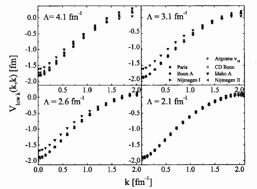
Figure 11: Diagonal matrix elements of $V_{\rm low-{\it k}}$ for different high-precision potentials in the ${}^{1}S_{0}$ partial wave with various cutoffs $\Lambda$.

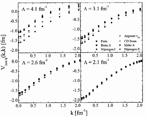
Figure 12: Diagonal matrix elements of $V_{\rm low-{\it k}}$ for different high-precision potentials in the ${}^{3}S_{1}$ partial wave with various cutoffs $\Lambda$.

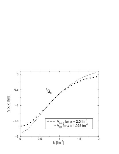
Figure 13: The ${}^{1}S_{0}$ diagonal matrix elements of $V_{\rm low-{\it k}}$ and the Kallio-Kolltveit potential for a configuration space cutoff of 1.025 fm.

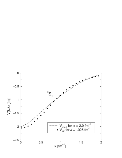
Figure 14: The ${}^{3}S_{1}$ diagonal matrix elements of $V_{\rm low-{\it k}}$ and the Kallio-Kolltveit potential for a configuration space cutoff of 1.025 fm.

Now the above renormalization group calculations were all carried out in momentum space. What is the relation of $V_{\rm low-{\it k}}$ to the effective interaction of eq. (49)? Although in the Mozskowski-Scott method the separation distance $d$ should be obtained separately for each channel, for comparison with $V_{\rm low-{\it k}}$ (which has the same momentum cutoff in all channels) it is most convenient to determine it for the ${}^{1}S_{0}$ channel ($d=1.025$) and then use the same $d$ in the ${}^{3}S_{1}$ channel. We show a comparison between $V_{\rm low-{\it k}}$ and the $G$ of eq. (49) in Figs. 14 and 14.

In Fig. 15 we show the diagonal matrix elements of the Kallio-Kolltveit potential, essentially the $G$ of eq. (49). Note that although the separation of short and long distance was made in configuration space, there are essentially no Fourier components above $k\sim 2\mbox{ fm}^{-1}$ in momentum space.

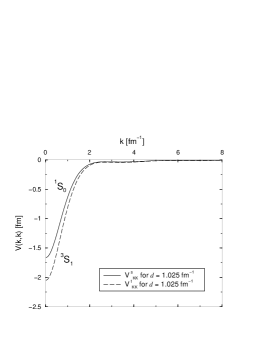
Figure 15: Diagonal matrix elements of the long-distance Kallio-Kolltveit potential $v_{l}$, including momenta above the $V_{\rm low-{\it k}}$ cutoff of 2.1 fm^-1.

It is, therefore, clear that the $G$ of eq. (49) that Bethe ended with is essentially $V_{\rm low-{\it k}}$, the only difference being that he made the separation of scales in configuration space whereas in $V_{\rm low-{\it k}}$ it is made in momentum space. Thus, we believe that Hans Bethe arrived at the right answer in “The Nuclear Many Body Problem,” but only much later did research workers use it to fit spectra.

References

- [1] N. Bohr, Nature 137 (1936) 344.
- [2] N. Bohr, Phi. Mag. 26 (1913) 476.
- [3] M. G. Mayer, Phys. Rev. 75 (1949) 1969.
- [4] O. Haxel, J. H. D. Jensen, and H. E. Suess, Z. Phys. 128 (1950) 295.
- [5] H. A. Bethe and R. F. Bacher, Rev. Mod. Phys. 8 (1936) 82.
- [6] R. Jastrow, Phys. Rev. 81 (1951) 165.
- [7] B. A. Lippmann and J. Schwinger, Phys. Rev. 79 (1950) 469.
- [8] K. M. Watson, Phys. Rev. 89 (1953) 575.
- [9] N. C. Francis and K. M. Watson, Phys. Rev. 92 (1953) 291.
- [10] S. K. Bogner, T. T. S. Kuo, and A. Schwenk, Phys. Rep. 386 (2003) 1.
- [11] G. E. Brown and M. Rho, Phys. Rep. 396 (2004) 1.
- [12] H. Feshbach, C. E. Porter, and V. F. Weisskopf, Phys. Rev. 96 (1954) 448.
- [13] G. E. Brown, Rev. Mod. Phys. 31 (1959) 893.
- [14] H. A. Bethe, Phys. Rev. 103 (1956) 1353.
- [15] K. A. Brueckner and C. A. Levinson, Phys. Rev. 97 (1955) 1344.
- [16] H. A. Bethe and J. Goldstone, Proc. Roy. Soc. A238 (1957) 551.
- [17] H. A. Bethe, B. H. Brandow, and A. G. Petschek, Phys. Rev. 129 (1963) 225.
- [18] S. A. Moszkowski and B. L. Scott, Ann. Phys. 14 (1961) 107.
- [19] H. A. Bethe, Phys. Rev. 76 (1949) 38.
- [20] G. E. Brown and A. D. Jackson, The Nucleon-Nucleon Interaction (North Holland, Amsterdam, 1976).
- [21] T. T. S. Kuo and G. E. Brown, Nucl. Phys. 85 (1966) 40.
- [22] H. A. Bethe, Phys. Rev. 138 (1965) B804.
- [23] R. Rajaraman, Phys. Rev. 129 (1963) 265.
- [24] L. D. Fadeev, Dokl. Akad. Nauk SSSR 138 (1961) 565; Sov. Phys. Doklady 6 (1961) 384.
- [25] G. Breit, Phys. Rev. 120 (1960) 287.
- [26] S. N. Gupta, Phys. Rev. 117 (1960) 1146.
- [27] A. Kallio and K. Kolltveit, Nucl. Phys. 53 (1964) 87.