Symmetries in physics

Abstract

The concept of symmetries in physics is briefly reviewed. In the first part of these lecture notes, some of the basic mathematical tools needed for the understanding of symmetries in nature are presented, namely group theory, Lie groups and Lie algebras, and Noether’s theorem. In the second part, some applications of symmetries in physics are discussed, ranging from isospin and flavor symmetry to more recent developments involving the interacting boson model and its extension to supersymmetries in nuclear physics.

1 Introduction

Symmetry and its mathematical framework—group theory—play an increasingly important role in physics. Both classical and quantum systems usually display great complexity, but the analysis of their symmetry properties often gives rise to simplifications and new insights which can lead to a deeper understanding. In addition, symmetries themselves can point the way toward the formulation of a correct physical theory by providing constraints and guidelines in an otherwise intractable situation. It is remarkable that, in spite of the wide variety of systems one may consider, all the way from classical ones to molecules, nuclei, and elementary particles, group theory applies the same basic principles and extracts the same kind of useful information from all of them. This universality in the applicability of symmetry considerations is one of the most attractive features of group theory. Most people have an intuitive understanding of symmetry, particularly in its most obvious manifestation in terms of geometric transformations that leave a body or system invariant. This interpretation, however, is not enough to readily grasp its deep connections with physics, and it thus becomes necessary to generalize the notion of symmetry transformations to encompass more abstract ideas. The mathematical theory of these transformations is the subject matter of group theory.

Group theory was developed in the beginning of the 19th century by Evariste Galois (1811-1832) who pointed out the relation between the existence of algebraic solutions of a polynomial equation and the group of permutations associated with the equation. Another important contribution was made in the 1870’s by Sophus Lie (1842-1899) who studied the mathematical theory of continuous transformations which led to the introduction of the basic concepts and operations of what are now known as Lie groups and Lie algebras. The deep connection between the abstract world of symmetries and dynamics—forces and motion and the fundamental laws of nature—was elucidated by Emmy Noether (1882-1935) in the early 20th century [1].

The concept of symmetry has played a major role in physics, especially in the 20th century with the development of quantum mechanics and quantum field theory. There is an enormously wide range of applications of symmetries in physics. Some of the most important ones are listed below [2].

• Geometric symmetries describe the arrangement of constituent particles into a geometric structure, for example the atoms in a molecule.

• Permutation symmetries in quantum mechanics lead to Fermi-Dirac and Bose-Einstein statistics for a system of identical particles with half-integer spin (fermions) and integer spin (bosons), respectively.

• Space-time symmetries fix the form of the equations governing the motion of the constituent particles. For example, the form of the Dirac equation for a relativistic spin-1/2 particle

  $$(i\gamma^{\mu}\partial_{\mu}-m)\psi(x)=0$$

  is determined by Lorentz invariance.

• Gauge symmetries fix the form of the interaction between constituent particles and external fields. For example, the form of the Dirac equation for a relativistic spin-1/2 particle in an external electromagnetic field $A_{\mu}$

  $$\left[\gamma^{\mu}(i\partial_{\mu}-eA_{\mu})-m\right]\psi(x)=0$$

  is dictated by the gauge symmetry of the electromagnetic interaction. The (electro-)weak and strong interactions are also governed by gauge symmetries.

• Dynamical symmetries fix the form of the interactions between constituent particles and/or external fields and determine the spectral properties of quantum systems. An early example was discussed by Pauli in 1926 [3] who recognized that the Hamiltonian of a particle in a Coulomb potential is invariant under four-dimensional rotations generated by the angular momentum and the Runge-Lenz vector.

These lectures notes are organized as follows. In the first part, a brief review is given of some of the basic mathematical concepts needed for the understanding of symmetries in nature, namely that of group theory, Lie groups and Lie algebras, and Noether’s theorem. In the second part, these ideas are illustrated by some applications in physics, ranging from isospin and flavor symmetry to more recent developments involving the interacting boson model and its extension to supersymmetries in nuclear physics. Some recent review articles on the concept of symmetries in physics are [2, 4, 5].

2 Elements of group theory

In this section, some general properties of group theory are reviewed. For a more thorough discussion of the basic concepts and its properties, the reader is referred to the literature [6, 7, 8, 9, 10, 11, 12].

2.1 Definition of a group

The concept of a group was introduced by Galois in a study of the existence of algebraic solutions of a polynomial equations. An abstract group $G$ is defined by a set of elements ($\hat{G}_{i},\hat{G}_{j},\hat{G}_{k},\ldots$) for which a “multiplication” rule (indicated here by $\circ$) combining these elements exists and which satisfies the following conditions.

• Closure.
  If $\hat{G}_{i}$ and $\hat{G}_{j}$ are elements of the set, so is their product $\hat{G}_{i}\circ\hat{G}_{j}~{}.$

• Associativity.
  The following property is always valid:

  $$\hat{G}_{i}\circ(\hat{G}_{j}\circ\hat{G}_{k})=(\hat{G}_{i}\circ\hat{G}_{j})\circ\hat{G}_{k}~{}.$$

• Identity.
  There exists an element $\hat{E}$ of $G$ satisfying

  $$\hat{E}\circ\hat{G}_{i}=\hat{G}_{i}\circ\hat{E}=\hat{G}_{i}~{}.$$

• Inverse.
  For every $\hat{G}_{i}$ there exists an element $\hat{G}_{i}^{-1}$ such that

  $$\hat{G}_{i}\circ\hat{G}_{i}^{-1}=\hat{G}_{i}^{-1}\circ\hat{G}_{i}=\hat{E}~{}.$$

The number of elements is called the order of the group. If in addition the elements of a group satisfy the condition of commutativity, the group is called an Abelian group.

• Commutativity.
  All elements obey

  $$\hat{G}_{i}\circ\hat{G}_{j}=\hat{G}_{j}\circ\hat{G}_{i}~{}.$$

2.2 Lie groups and Lie algebras

For continuous (or Lie) groups all elements may be obtained by exponentiation in terms of a basic set of elements $\hat{g}_{i}$, $i=1,2,\dots,s$, called generators, which together form the Lie algebra associated with the Lie group. A simple example is provided by the group of rotations in two-dimensional space, with elements that may be realized as

$$\hat{G}(\alpha)=\exp[-i\alpha\hat{l}_{z}]~{},$$ (1)

where $\alpha$ is the angle of rotation and

$$\hat{l}_{z}=-i\left(x{\frac{\partial}{\partial y}}-y{\frac{\partial}{\partial x}}\right)~{},$$ (2)

is the generator of these transformations in the $x$–$y$ plane. Three-dimensional rotations require the introduction of two additional generators, associated with rotations in the $z$–$x$ and $y$–$z$ planes,

$$\hat{l}_{y}=-i\left(z{\frac{\partial}{\partial x}}-x{\frac{\partial}{\partial z}}\right)~{},\qquad\hat{l}_{x}=-i\left(y{\frac{\partial}{\partial z}}-z{\frac{\partial}{\partial y}}\right)~{},$$ (3)

Finite rotations can then be parametrized by three angles (which may be chosen to be the Euler angles) and expressed as a product of exponentials of the generators of Eqs. (2) and (3). Evaluating the commutators of these operators, we find

$$[\hat{l}_{x},\hat{l}_{y}]=i\hat{l}_{z}~{},\qquad[\hat{l}_{y},\hat{l}_{z}]=i\hat{l}_{x}~{},\qquad[\hat{l}_{z},\hat{l}_{x}]=i\hat{l}_{y}~{},$$ (4)

which illustrates the closure property of the group generators. In general, the operators $\hat{g}_{i}$, $i=1,2,\dots,s$, define a Lie algebra if they close under commutation

$$[\hat{g}_{i},\hat{g}_{j}]=\sum_{k}c^{k}_{ij}\hat{g}_{k}~{},$$ (5)

and satisfy the Jacobi identity

$$[\hat{g}_{i},[\hat{g}_{j},\hat{g}_{k}]]+[\hat{g}_{k},[\hat{g}_{i},\hat{g}_{j}]]+[\hat{g}_{j},[\hat{g}_{k},\hat{g}_{i}]]=0~{}.$$ (6)

The constants $c^{k}_{ij}$ are called structure constants, and determine the properties of both the Lie algebra and its associated Lie group. Lie groups have been classified by Cartan, and many of their properties have been established.

The group of unitary transformations in $n$ dimensions is denoted by $U(n)$ and of rotations in $n$ dimensions by $SO(n)$ (Special Orthogonal). The corresponding Lie algebras are sometimes indicated by lower case symbols, $u(n)$ and $so(n)$, respectively.

2.3 Symmetries and conservation laws

Symmetry in physics is expressed by the invariance of a Lagrangian or of a Hamiltonian or, equivalently, of the equations of motion, with respect to some group of transformations. The connection between the abstract concept of symmetries and dynamics is formulated as Noether’s theorem which says that, irrespective of a classical or a quantum mechanical treatment, an invariant Lagrangian or Hamiltonian with respect to a continuous symmetry implies a set of conservation laws [13]. For example, the conservation of energy, momentum and angular momentum are a consequence of the invariance of the system under time translations, space translations and rotations, respectively.

In quantum mechanics, continuous symmetry transformations can in general be expressed as

$$U=\exp\left[i\sum_{j}\alpha_{j}\hat{g}_{j}\right]~{}.$$ (7)

States and operators transform as

$$\left|\psi\right>\rightarrow\left|\psi^{\prime}\right>=U\left|\psi\right>~{},\hskip 28.45274ptA\rightarrow A^{\prime}=UAU^{\dagger}~{}.$$ (8)

For the Hamiltonian one then has

$$H\rightarrow H^{\prime}=UHU^{\dagger}=H+i\sum_{j}\alpha_{j}[\hat{g}_{j},H]+{\cal O}(\alpha^{2})~{}.$$ (9)

When the physical system is invariant under the symmetry transformations $U$, the Hamiltonian remains the same $H^{\prime}=H$. Therefore, the Hamiltonian commutes with the generators of the symmetry transformation

$$\left[\hat{g}_{j},H\right]=0~{},$$ (10)

which implies that the generators are constants of the motion. Eq. (10), together with the closure relation of the generators of Eq. (5), constitutes the definition of the symmetry algebra for a time-independent system.

2.4 Constants of the motion and state labeling

For any Lie algebra one may construct one or more operators $\hat{\cal C}_{l}$ which commute with all the generators $\hat{g}_{j}$

$$[\hat{\cal C}_{l},\hat{g}_{j}]=0,\qquad l=1,2,\dots,r,\quad j=1,2,\dots,s~{}.$$ (11)

These operators are called Casimir operators or Casimir invariants. They may be linear, quadratic, or higher order in the generators. The number $r$ of linearly independent Casimir operators is called the rank of the algebra [9]. This number coincides with the maximum subset of generators which commute among themselves (called weight generators)

$$[\hat{g}_{\alpha},\hat{g}_{\beta}]=0~{},\qquad\alpha,\beta=1,2,\dots,r~{},$$ (12)

where greek labels were used to indicate that they belong to the subset satisfying Eq. (12). The operators $(\hat{\cal C}_{l}$, $\hat{g}_{\alpha})$ may be simultaneously diagonalized and their eigenvalues used to label the corresponding eigenstates.

To illustrate these definitions, we consider the $su(2)$ algebra $(\hat{j}_{x}$, $\hat{j}_{y}$, $\hat{j}_{z})$ with commutation relations

$$[\hat{j}_{x},\hat{j}_{y}]=i\hat{j}_{z}~{},\qquad[\hat{j}_{z},\hat{j}_{x}]=i\hat{j}_{y}~{},\qquad[\hat{j}_{y},\hat{j}_{z}]=i\hat{j}_{x}~{},$$ (13)

which is isomorphic to the $so(3)$ commutators given in Eq. (4). From Eq. (13) one can conclude that the rank of the algebra is $r=1$. Therefore one can choose $\hat{j}_{z}$ as the generator to diagonalize together with the Casimir invariant

$$\hat{j}^{2}=\hat{j}^{2}_{x}+\hat{j}^{2}_{y}+\hat{j}^{2}_{z}~{}.$$ (14)

The eigenvalues and branching rules for the commuting set $(\hat{\cal C}_{l}$, $\hat{g}_{\alpha})$ can be determined solely from the commutation relations Eq. (5). In the case of $su(2)$ the eigenvalue equations are

$$\hat{j}^{2}|jm\rangle=n_{j}|jm\rangle~{},\qquad\hat{j}_{z}|jm\rangle=m|jm\rangle~{},$$ (15)

where $j$ is an index to distinguish the different $\hat{j}^{2}$ eigenvalues. Defining the raising and lowering operators

$$\hat{j}_{\pm}=\hat{j}_{x}\pm i\hat{j}_{y}~{},$$ (16)

and using Eq. (13), one finds the well-known results

$$n_{j}=j(j+1)~{},\qquad j=0,\frac{1}{2},1,\ldots,\qquad m=-j,-j+1,\ldots,j~{}.$$ (17)

As a bonus, the action of $\hat{j}_{\pm}$ on the $|jm\rangle$ eigenstates is determined to be

$$\hat{j}_{\pm}|jm\rangle=\sqrt{(j\mp m)(j\pm m+1)}|jm\pm 1\rangle~{}.$$ (18)

In the case of a general Lie algebra, see Eq. (5), this procedure becomes quite complicated, but it requires the same basic steps. The analysis leads to the algebraic determination of eigenvalues, branching rules, and matrix elements of raising and lowering operators [9].

The symmetry algebra provides constants of the motion, which in turn lead to quantum numbers that label the states associated with a given energy eigenvalue. The raising and lowering operators in this algebra only connect degenerate states. The dynamical algebra, however, defines the whole set of eigenstates associated with a given system. The generators are no longer constants of the motion as not all commute with the Hamiltonian. The raising and lowering operators may now connect all states with each other.

2.5 Dynamical symmetries

In this section we show how the concepts presented in the previous sections lead to an algebraic approach which can be applied to the study of different physical systems. We start by considering again Eq. (10) which describes the invariance of a Hamiltonian under the algebra $g\equiv(\hat{g}_{j})$

$$[H,\hat{g}_{j}]=0~{},$$ (19)

implying that $g$ plays the role of symmetry algebra for the system. An eigenstate of $H$ with energy $E$ may be written as $|\Gamma\gamma\rangle$, where $\Gamma$ labels the irreducible representations of the group $G$ corresponding to $g$ and $\gamma$ distinguishes between the different eigenstates with energy $E$ (and may be chosen to correspond to irreducible representations of subgroups of $G$). The energy eigenvalues of the Hamiltonian in Eq. (19) thus depend only on $\Gamma$

$$H|\Gamma\gamma\rangle=E(\Gamma)|\Gamma\gamma\rangle~{}.$$ (20)

The generators $\hat{g}_{j}$ do not admix states with different $\Gamma$’s.

Let’s now consider the chain of algebras

$$g_{1}\supset g_{2}~{},$$ (21)

which will lead to the introduction of the concept of dynamical symmetry. Here $g_{2}$ is a subalgebra of $g_{1}$, $g_{2}\subset g_{1}$, i.e. its generators form a subset of the generators of $g_{1}$ and close under commutation. If $g_{1}$ is a symmetry algebra for $H$, its eigenstates can be labeled as $|\Gamma_{1}\gamma_{1}\rangle$. Since $g_{2}\subset g_{1}$, $g_{2}$ must also be a symmetry algebra for $H$ and, consequently, its eigenstates labeled as $|\Gamma_{2}\gamma_{2}\rangle$. Combination of the two properties leads to the eigenequation

$$H|\Gamma_{1}\Gamma_{2}\gamma_{2}\rangle=E(\Gamma_{1})|\Gamma_{1}\Gamma_{2}\gamma_{2}\rangle~{},$$ (22)

where the role of $\gamma_{1}$ is played by $\Gamma_{2}\gamma_{2}$ and hence the eigenvalues depend only on $\Gamma_{1}$. This process may be continued when there are further subalgebras, that is, $g_{1}\supset g_{2}\supset g_{3}\supset\cdots$, in which case $\gamma_{2}$ is substituted by $\Gamma_{3}\gamma_{3}$, and so on.

In many physical applications the original assumption that $g_{1}$ is a symmetry algebra of the Hamiltonian is found to be too strong and must be relaxed, that is, one is led to consider the breaking of this symmetry. An elegant way to do so is by considering a Hamiltonian of the form

$$H^{\prime}=a\,\hat{\cal C}_{l_{1}}(g_{1})+b\,\hat{\cal C}_{l_{2}}(g_{2})~{},$$ (23)

where $\hat{\cal C}_{l_{i}}(g_{i})$ is a Casimir invariant of $g_{i}$. Since $[H^{\prime},\hat{g}_{i}]=0$ for $\hat{g}_{i}\in g_{2}$, $H^{\prime}$ is invariant under $g_{2}$, but not anymore under $g_{1}$ because $[\hat{\cal C}_{l_{2}}(g_{2}),\hat{g}_{i}]\neq 0$ for $\hat{g}_{i}\not\in g_{2}$. The new symmetry algebra is thus $g_{2}$ while $g_{1}$ now plays the role of dynamical algebra for the system, as long as all states we wish to describe are those originally associated with $E(\Gamma_{1})$. The extent of the symmetry breaking depends on the ratio $b/a$. Furthermore, since $H^{\prime}$ is given as a combination of Casimir operators, its eigenvalues can be obtained in closed form

$$H^{\prime}|\Gamma_{1}\Gamma_{2}\gamma_{2}\rangle=\left[a\,E_{l_{1}}(\Gamma_{1})+b\,E_{l_{2}}(\Gamma_{2})\right]|\Gamma_{1}\Gamma_{2}\gamma_{2}\rangle~{}.$$ (24)

The kind of symmetry breaking caused by interactions of the form (23) is known as dynamical-symmetry breaking and the remaining symmetry is called a dynamical symmetry of the Hamiltonian $H^{\prime}$. From Eq. (24) one concludes that even if $H^{\prime}$ is not invariant under $g_{1}$, its eigenstates are the same as those of $\hat{H}$ in Eq. (22). The dynamical-symmetry breaking thus splits but does not admix the eigenstates.

In the last part of these lecture notes, we discuss some applications of the algebraic approach in nuclear and particle physics. The algebraic approach, both in the sense we have defined here and in its generalizations to other fields of research, has become an important tool in the search for a unified description of physical phenomena.

3 Isospin symmetry

Some of these ideas can be illustrated with well-known examples. In 1932 Heisenberg considered the occurrence of isospin multiplets in nuclei [14]. To a good approximation, the strong interaction between nucleons does not distinguish between protons and neutrons. In the isospin formalism, the proton and neutron are treated as one and the same particle: the nucleon with isospin $t=\frac{1}{2}$. The isospin projections $m_{t}=+\frac{1}{2}$ and $-\frac{1}{2}$ are identified with the proton and the neutron, respectively. The total isospin of the nucleus is denoted by $T$ and its projection by $M_{T}$. In the notation used above (without making the distinction between algebras and groups), $G_{1}$ is in this case the isospin group $SU_{T}(2)$ generated by the operators $\hat{T}_{x}$, $\hat{T}_{y}$, and $\hat{T}_{z}$ which satisfy commutation relations of Eq. (13), and $G_{2}$ can be identified with $SO_{T}(2)$ generated by $\hat{T}_{z})$. An isospin-invariant Hamiltonian commutes with $\hat{T}_{x}$, $\hat{T}_{y}$, and $\hat{T}_{z}$, and hence the eigenstates $|TM_{T}\rangle$ with fixed $T$ and $M_{T}=-T,-T+1,\ldots,T$ are degenerate in energy. However, the electromagnetic interaction breaks isospin invariance due to difference in electric charge of the proton and the neutron, and lifts the degeneracy of the states $|TM_{T}\rangle$. It is assumed that this symmetry breaking occurs dynamically, and since the Coulomb force has a two-body character, the breaking terms are at most quadratic in $\hat{T}_{z}$ [10]. The energies of the corresponding nuclear states with the same $T$ are then given by

$$E(M_{T})=a+b\,M_{T}+c\,M_{T}^{2}~{},$$ (25)

and $SU_{T}(2)$ becomes the dynamical symmetry for the system while $SO_{T}(2)$ is the symmetry algebra. The dynamical symmetry breaking thus implied that the eigenstates of the nuclear Hamiltonian have well-defined values of $T$ and $M_{T}$. Extensive tests have shown that indeed this is the case to a good approximation, at least at low excitation energies and in light nuclei [15]. Eq. (25) can be tested in a number of cases. In Figure 1 a $T=3/2$ multiplet consisting of states in the nuclei ¹³B, ¹³C, ¹³N, and ¹³O is compared with the theoretical prediction of Eq. (25).

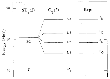
Figure 1: Binding energies of the $T=3/2$ isobaric analog states with angular momentum and parity $J^{\pi}=1/2^{-}$ in ¹³B, ¹³C, ¹³N, and ¹³O. The column on the left is obtained for an exact $SU_{T}(2)$ symmetry, which predicts states with different $M_{T}$ to be degenerate. The middle column is obtained in the case of an $SU_{T}(2)$ dynamical symmetry, Eq. (25) with parameters $a=80.59$, $b=-2.96$, and $c=-0.26$ MeV.

4 Flavor symmetry

A less trivial example of dynamical-symmetry breaking is provided by the Gell-Mann–Okubo mass-splitting formula for elementary particles [16, 17]. In the previous example, we saw that the near equality of the neutron and proton masses suggested the existence of isospin multiplets which was later confirmed at higher energies for other particles. Gell-Mann and Ne’eman proposed independently a dynamical algebra to further classify and order these different isospin multiplets of hadrons in terms of $SU(3)$ representations [18] . Baryons were found to occur in decuplets, octets and singlets, whereas mesons appear only in octets and singlets. The members of a $SU(3)$ multiplet are labeled by their isospin $T$, $M_{T}$ and hypercharge $Y$ quantum numbers, according to the group chain

$$\begin{array}[]{ccccccccc}SU(3)&\supset&U_{Y}(1)&\otimes&SU_{T}(2)&\supset&U_{Y}(1)&\otimes&SO_{T}(2)\\ \downarrow&&\downarrow&&\downarrow&&&&\downarrow\\ (\lambda,\mu)&&Y&&T&&&&M_{T}\end{array}$$ (26)

If one would assume $SU(3)$ invariance, all particles in a multiplet would have the same mass, but since the experimental masses of other baryons differ from the nucleon masses by hundreds of MeV, the $SU(3)$ symmetry clearly must be broken.

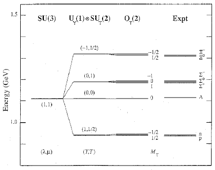
Figure 2: Mass spectrum of the ground state baryon octet. The column on the left is obtained for an exact $SU(3)$ symmetry, which predicts all masses to be the same, while the next two columns represent successive breakings of this symmetry in a dynamical manner. The column under $SO_{T}(2)$ is obtained with Eq. (29) with parameters $a=1111.3$, $b=-189.6$, $d=-39.9$, $e=-3.8$, and $f=0.9$ MeV.

Dynamical symmetry breaking allows the baryon states to still be classified by Eq. (26). Following the procedure outlined above and keeping up to quadratic terms, one finds a mass operator of the form

$$\hat{M} = a+b\,\hat{\cal C}_{1U_{Y}(1)}+c\,\hat{\cal C}^{2}_{1U_{Y}(1)}+d\,\hat{\cal C}_{2SU_{T}(2)}+e\,\hat{\cal C}_{1SO_{T}(2)}+f\,\hat{\cal C}^{2}_{1SO_{T}(2)}~{},$$ (27)

with eigenvalues

$$M(Y,T,M_{T})=a+b\,Y+c\,Y^{2}+d\,T(T+1)+e\,M_{T}+f\,M_{T}^{2}~{}.$$ (28)

A further assumption regarding the $SU(3)$ tensor character of the strong interaction [16, 17] leads to a relation between the coefficients $c$ and $d$ in Eq. (28), $c=-d/4$

$$M^{\prime}(Y,T)=a+b\,Y+d\left[T(T+1)-\frac{1}{4}Y^{2}\right]+e\,M_{T}+f\,M_{T}^{2}~{}.$$ (29)

If one neglects the isospin breaking due to the last two terms, one recovers the Gell-Mann-Okubo mass formula. In Figure 2 this process of successive dynamical-symmetry breaking is illustrated with the octet representation containing the neutron and the proton and the $\Lambda$, $\Sigma$, and $\Xi$ baryons.

5 Nuclear supersymmetry

Nuclear supersymmetry (n-SUSY) is a composite-particle phenomenon, linking the properties of bosonic and fermionic systems, framed in the context of the Interacting Boson Model of nuclear structure [19]. Composite particles, such as the $\alpha$-particle are known to behave as approximate bosons. As He atoms they become superfluid at low temperatures, an under certain conditions can also form Bose-Einstein condensates. At higher densities (or temperatures) the constituent fermions begin to be felt and the Pauli principle sets in. Odd-particle composite systems, on the other hand, behave as approximate fermions, which in the case of the Interacting Boson-Fermion Model are treated as a combination of bosons and an (ideal) fermion [20]. In contrast to the theoretical construct of supersymmetric particle physics, where SUSY is postulated as a generalization of the Lorentz-Poincare invariance at a fundamental level, experimental evidence has been found for n-SUSY [21, 22, 23, 24, 25, 26, 27] as we shall discuss below. Nuclear supersymmetry should not be confused with fundamental SUSY, which predicts the existence of supersymmetric particles, such as the photino and the selectron for which, up to now, no evidence has been found. If such particles exist, however, SUSY must be strongly broken, since large mass differences must exist among superpartners, or otherwise they would have been already detected. Nuclear supersymmetry, on the other hand, is a theory that establishes precise links among the spectroscopic properties of certain neighboring nuclei. Even-even and odd-odd nuclei are composite bosonic systems, while odd-$A$ nuclei are fermionic. It is in this context that n-SUSY provides a theoretical framework where bosonic and fermionic systems are treated as members of the same supermultiplet [23]. Nuclear supersymmetry treats the excitation spectra and transition intensities of the different nuclei as arising from a single Hamiltonian and a single set of transition operators. Nuclear supersymmetry was originally postulated as a symmetry among pairs of nuclei [21, 22, 23], and was subsequently extended to quartets of nuclei, where odd-odd nuclei could be incorporated in a natural way [28]. Evidence for the existence of n-SUSY (albeit possibly significantly broken) grew over the years, specially for the quartet of nuclei ¹⁹⁴Pt, ¹⁹⁵Au, ¹⁹⁵Pt and ¹⁹⁶Au, but only recently more systematic evidence was found [25, 26, 27].

We first present a pedagogic review of dynamical (super)symmetries in even- and odd-mass nuclei, which is based in part on [24]. Next we discuss the generalization of these concepts to include the neutron-proton degree of freedom.

5.1 Dynamical symmetries in even-even nuclei

Dynamical supersymmetries were introduced [21] in nuclear physics in 1980 by Franco Iachello in the context of the Interacting Boson Model (IBM) and its extensions. The spectroscopy of atomic nuclei is characterized by the interplay between collective (bosonic) and single-particle (fermionic) degrees of freedom.

The IBM describes collective excitations in even-even nuclei in terms of a system of interacting monopole and quadrupole bosons with angular momentum $l=0,2$ [19]. The bosons are associated with the number of correlated proton and neutron pairs, and hence the number of bosons $N$ is half the number of valence nucleons. Since it is convenient to express the Hamiltonian and other operators of interest in second quantized form, we introduce creation, $s^{\dagger}$ and $d^{\dagger}_{m}$, and annihilation, $s$ and $d_{m}$, operators, which altogether can be denoted by $b^{\dagger}_{i}$ and $b_{i}$ with $i=l,m$ ($l=0,2$ and $-l\leq m\leq l$). The operators $b^{\dagger}_{i}$ and $b_{i}$ satisfy the commutation relations

$$[b_{i},b^{\dagger}_{j}]\;=\;\delta_{ij}~{},\hskip 28.45274pt[b^{\dagger}_{i},b^{\dagger}_{j}]\;=\;[b_{i},b_{j}]\;=\;0~{}.$$ (30)

The bilinear products

$$B_{ij}\;=\;b^{\dagger}_{i}b_{j}~{},$$ (31)

generate the algebra of $U(6)$ the unitary group in 6 dimensions

$$[B_{ij},B_{kl}]\;=\;B_{il}\,\delta_{jk}-B_{kj}\,\delta_{il}~{}.$$ (32)

We want to construct states and operators that transform according to irreducible representations of the rotation group (since the problem is rotationally invariant). The creation operators $b^{\dagger}_{i}$ transform by definition as irreducible tensors under rotation. However, the annihilation operators $b_{i}$ do not. It is an easy exercise to contruct operators that do transform appropriately

$$\tilde{b}_{lm}\;=\;(-)^{l-m}b_{l,-m}~{}.$$ (33)

The 36 generators of Eq. (31) can be rewritten in angular-momentum-coupled form as

$$[b^{\dagger}_{l}\times\tilde{b}_{l^{\prime}}]^{(L)}_{M}\;=\;\sum_{mm^{\prime}}\langle l,m,l^{\prime},m^{\prime}|L,M\rangle\,b^{\dagger}_{lm}\tilde{b}_{l^{\prime}m^{\prime}}~{}.$$ (34)

The one- and two-body Hamiltonian can be expressed in terms of the generators of $U(6)$ as

$$H = \sum_{l}\epsilon_{l}\sum_{m}b^{\dagger}_{lm}b_{lm}$$ (35)

$$+\sum_{L}\sum_{l_{1}l_{2}l_{3}l_{4}}u^{(L)}_{l_{1}l_{2}l_{3}l_{4}}\,[[b^{\dagger}_{l_{1}}\times\tilde{b}_{l_{2}}]^{(L)}\times[b^{\dagger}_{l_{3}}\times\tilde{b}_{l_{4}}]^{(L)}]^{(0)}~{}.$$

In general, the Hamiltonian has to be diagonalized numerically to obtain the energy eigenvalues and wave functions. There exist, however, special situations in which the eigenvalues can be obtained in closed, analytic form. These special solutions provide a framework in which energy spectra and other nuclear properties (such as quadrupole transitions and moments) can be interpreted in a qualitative way. These situations correspond to dynamical symmetries of the Hamiltonian [19] (see section 2.5).

The concept of dynamical symmetry has been shown to be a very useful tool in different branches of physics. A well-known example in nuclear physics is the Elliott $SU(3)$ model [29] to describe the properties of light nuclei in the $sd$ shell. Another example is the $SU(3)$ flavor symmetry of Gell-Mann and Ne’eman [18] to classify the baryons and mesons into flavor octets, decuplets and singlets and to describe their masses with the Gell-Mann-Okubo mass formula, as described in the previous sections.

The group structure of the IBM Hamiltonian is that of $G=U(6)$. Since nuclear states have good angular momentum, the rotation group in three dimensions $SO(3)$ should be included in all subgroup chains of $G$ [19]

$$U(6)\supset\left\{\begin{array}[]{l}U(5)\supset SO(5)\supset SO(3)~{},\\ SU(3)\supset SO(3)~{},\\ SO(6)\supset SO(5)\supset SO(3)~{}.\end{array}\right.$$ (39)

The three dynamical symmetries which correspond to the group chains in Eq. (39) are limiting cases of the IBM and are usually referred to as the $U(5)$ (vibrator), the $SU(3)$ (axially symmetric rotor) and the $SO(6)$ ($\gamma$-unstable rotor).

Here we consider a simplified form of the general expression of the IBM Hamiltonian of Eq. (35) that contains the main features of collective motion in nuclei

$$H\;=\;\epsilon\,\hat{n}_{d}-\kappa\,\hat{Q}(\chi)\cdot\hat{Q}(\chi)~{},$$ (40)

where $n_{d}$ counts the number of quadrupole bosons

$$\hat{n}_{d}\;=\;\sqrt{5}\,[d^{\dagger}\times\tilde{d}]^{(0)}\;=\;\sum_{m}d^{\dagger}_{m}d_{m}~{},$$ (41)

and $Q$ is the quadrupole operator

$$\hat{Q}_{m}(\chi)\;=\;[s^{\dagger}\times\tilde{d}+d^{\dagger}\times\tilde{s}+\chi\,d^{\dagger}\times\tilde{d}]^{(2)}_{m}~{}.$$ (42)

The three dynamical symmetries are recovered for different choices of the coefficients $\epsilon$, $\kappa$ and $\chi$. Since the IBM Hamiltonian conserves the number of bosons and is invariant under rotations, its eigenstates can be labeled by the total number of bosons $N$ and the angular momentum $L$.

The $U(5)$ limit. In the absence of a quadrupole-quadrupole interaction $\kappa=0$, the Hamiltonian of Eq. (40) becomes proportional to the linear Casimir operator of $U(5)$

$$H_{1}\;=\;\epsilon\,\hat{n}_{d}\;=\;\epsilon\,\hat{\cal C}_{1U(5)}~{}.$$ (43)

In addition to $N$ and $L$, the basis states can be labeled by the quantum numbers $n_{d}$ and $\tau$, which characterize the irreducible representations of $U(5)$ and $SO(5)$. Here $n_{d}$ represents the number of quadrupole bosons and $\tau$ the boson seniority. The eigenvalues of $H_{1}$ are given by the expectation value of the Casimir operator

$$E_{1}\;=\;\epsilon\,n_{d}~{}.$$ (44)

In this case, the energy spectrum is characterized by a series of multiplets, labeled by the number of quadrupole bosons, at a constant energy spacing which is typical for a vibrational nucleus.

The $SU(3)$ limit. For the quadrupole-quadrupole interaction, we can distinguish two situations in which the eigenvalue problem can be solved analytically. If $\chi=\mp\sqrt{7}/2$, the Hamiltonian has a $SU(3)$ dynamical symmetry

$$H_{2}\;=\;-\kappa\,\hat{Q}(\mp\sqrt{7}/2)\cdot\hat{Q}(\mp\sqrt{7}/2)\;=\;-\frac{1}{2}\kappa\left[\hat{\cal C}_{2SU(3)}-\frac{3}{4}\hat{\cal C}_{2SO(3)}\right]~{}.$$ (45)

In this case, the eigenstates can be labeled by $(\lambda,\mu)$ which characterize the irreducible representations of $SU(3)$. The eigenvalues are

$$E_{2}\;=\;-\frac{1}{2}\kappa\left[\lambda(\lambda+3)+\mu(\mu+3)+\lambda\mu)-\frac{3}{4}\kappa L(L+1)\right]~{}.$$ (46)

The energy spectrum is characterized by a series of bands, in which the energy spacing is proportional to $L(L+1)$, as in the rigid rotor model. The ground state band has $(\lambda,\mu)=(2N,0)$ and the first excited band $(2N-4,2)$ corresponds to a degenerate $\beta$ and $\gamma$ band. The sign of the coefficient $\chi$ is related to a prolate (-) or an oblate (+) deformation.

The $SO(6)$ limit. For $\chi=0$, the Hamiltonian has a $SO(6)$ dynamical symmetry

$$H_{3}\;=\;-\kappa\,\hat{Q}(0)\cdot\hat{Q}(0)\;=\;-\kappa\left[\hat{\cal C}_{2SO(6)}-\hat{\cal C}_{2SO(5)}\right]~{}.$$ (47)

The basis states are labeled by $\sigma$ and $\tau$ which characterize the irreducible representations of $SO(6)$ and $SO(5)$, respectively. Characteristic features of the energy spectrum

$$E_{3}\;=\;-\kappa\left[\sigma(\sigma+4)-\tau(\tau+3)\right]~{},$$ (48)

are the repeating patterns $L=0,2,4,2$ which is typical of the $\gamma$-unstable rotor.

For other choices of the coefficients, the Hamiltonian of Eq. (40) describes situations in between any of the dynamical symmetries which correspond to transitional regions, e.g. the Pt-Os isotopes exhibit a transition between a $\gamma$-unstable and a rigid rotor $SO(6)\leftrightarrow SU(3)$, the Sm isotopes between vibrational and rotational nuclei $U(5)\leftrightarrow SU(3)$, and the Ru isotopes between vibrational and $\gamma$-unstable nuclei $U(5)\leftrightarrow SO(6)$ [19].

5.2 Dynamical symmetries in odd-$A$ nuclei

For odd-mass nuclei the IBM has been extended to include single-particle degrees of freedom [20]. The Interacting Boson-Fermion Model (IBFM) has as its building blocks a set of $N$ bosons with $l=0,2$ and an odd nucleon (either a proton or a neutron) occupuying the single-particle orbits with angular momenta $j=j_{1},j_{2},\dots$. The components of the fermion angular momenta span the $\Omega$-dimensional space of the group $U(\Omega)$ with $\Omega=\sum_{j}(2j+1)$.

One introduces, in addition to the boson creation $b^{\dagger}_{i}$ and annihilation $b_{i}$ operators for the collective degrees of freedom, fermion creation $a^{\dagger}_{\mu}$ and annihilation $a_{\mu}$ operators for the single-particle. The fermion operators satisfy anti-commutation relations

$$\{a_{\mu},a^{\dagger}_{\nu}\}\;=\;\delta_{\mu\nu}~{},\hskip 28.45274pt\{a^{\dagger}_{\mu},a^{\dagger}_{\nu}\}\;=\;\{a_{\mu},a_{\nu}\}\;=\;0~{}.$$ (49)

By construction the fermion operators commute with the boson operators. The bilinear products

$$A_{\mu\nu}\;=\;a^{\dagger}_{\mu}a_{\nu}~{},$$ (50)

generate the algebra of $U(\Omega)$, the unitary group in $\Omega$ dimensions

$$[A_{\mu\nu},A_{\rho\sigma}]\;=\;A_{\mu\sigma}\,\delta_{\nu\rho}-A_{\rho\nu}\,\delta_{\mu\sigma}~{}.$$ (51)

For the mixed system of boson and fermion degrees of freedom we introduce angular-momentum-coupled generators as

$$B^{(L)}_{M}(l,l^{\prime})\;=\;[b^{\dagger}_{l}\times\tilde{b}_{l^{\prime}}]^{(L)}_{M}~{},\hskip 28.45274ptA^{(L)}_{M}(j,j^{\prime})\;=\;[a^{\dagger}_{j}\times\tilde{a}_{j^{\prime}}]^{(L)}_{M}~{},$$ (52)

where $\tilde{a}_{jm}$ is defined to be a spherical tensor operator

$$\tilde{a}_{jm}\;=\;(-)^{j-m}a_{j,-m}~{}.$$ (53)

The most general one- and two-body rotational invariant Hamiltonian of the IBFM can be written as

$$H\;=\;H_{B}+H_{F}+V_{BF}~{},$$ (54)

where $H_{B}$ is the IBM Hamiltonian of Eq. (35), $H_{F}$ is the fermion Hamiltonian

$$H_{F} = \sum_{j}\eta_{j}\sum_{m}a^{\dagger}_{jm}a_{jm}$$ (55)

$$+\sum_{L}\sum_{j_{1}j_{2}j_{3}j_{4}}v^{(L)}_{j_{1}j_{2}j_{3}j_{4}}\,[[a^{\dagger}_{j_{1}}\times\tilde{a}_{j_{2}}]^{(L)}\times[a^{\dagger}_{j_{3}}\times\tilde{a}_{j_{4}}]^{(L)}]^{(0)}~{},$$

and $V_{BF}$ the boson-fermion interaction

$$V_{BF} = \sum_{L}\sum_{l_{1}l_{2}j_{1}j_{2}}w^{(L)}_{l_{1}l_{2}j_{1}j_{2}}\,[[b^{\dagger}_{l_{1}}\times\tilde{b}_{l_{2}}]^{(L)}\times[a^{\dagger}_{j_{1}}\times\tilde{a}_{j_{2}}]^{(L)}]^{(0)}~{}.$$ (56)

The IBFM Hamiltonian has an interesting algebraic structure, that suggests the possible occurrence of dynamical symmetries in odd-$A$ nuclei. Since in the IBFM odd-$A$ nuclei are described in terms of a mixed system of interacting bosons and fermions, the concept of dynamical symmetries has to be generalized. Under the restriction, that both the boson and fermion states have good angular momentum, the respective group chains should contain the rotation group ($SO(3)$ for bosons and $SU(2)$ for fermions) as a subgroup

$$U^{B}(6)\supset\cdots\supset SO^{B}(3)~{},$$

$$U^{F}(\Omega)\supset\cdots\supset SU^{F}(2)~{},$$ (57)

where we have introduced superscripts to distinguish between boson and fermion groups. If one of subgroups of $U^{B}(6)$ is isomorphic to one of the subgroups of $U^{F}(\Omega)$, the boson and fermion group chains can be combined into a common boson-fermion group chain. When the Hamiltonian is written in terms of Casimir invariants of the combined boson-fermion group chain, a dynamical boson-fermion symmetry arises.

The $Spin(6)$ limit. Among the many different possibilities, we consider two dynamical boson-fermion symmetries associated with the $SO(6)$ limit of the IBM. The first example discussed in the literature [21, 30] is the case of bosons with $SO(6)$ symmetry and the odd nucleon occupying a single-particle orbit with spin $j=3/2$. The relevant group chains are

$$U^{B}(6)\supset SO^{B}(6)\supset SO^{B}(5)\supset SO^{B}(3)~{},$$

$$U^{F}(4)\supset SU^{F}(4)\supset Sp^{F}(4)\supset SU^{F}(2)~{}.$$ (58)

Since $SO(6)$ and $SU(4)$ are isomorphic, the boson and fermion group chains can be combined into

$$U^{B}(6)\otimes U^{F}(4) \supset SO^{B}(6)\otimes SU^{F}(4)$$ (59)

$$\supset Spin(6)\supset Spin(5)\supset Spin(3)~{}.$$

The spinor groups $Spin(n)$ are the universal covering groups of the orthogonal groups $SO(n)$, with $Spin(6)\sim SU(4)$, $Spin(5)\sim Sp(4)$ and $Spin(3)\sim SU(2)$. The generators of the spinor groups consist of the sum of a boson and a fermion part. For example, for the quadrupole operator we have

$$\hat{Q}_{m}\;=\;[s^{\dagger}\times\tilde{d}+d^{\dagger}\times\tilde{s}]^{(2)}_{m}+[a^{\dagger}_{3/2}\times\tilde{a}_{3/2}]^{(2)}_{m}~{}.$$ (60)

We consider a simple quadrupole-quadrupole interaction which, just as for the $SO(6)$ limit of the IBM, can be written as the difference of two Casimir invariants

$$H\;=\;-\kappa\,\hat{Q}\cdot\hat{Q}\;=\;-\kappa\left[\hat{\cal C}_{2Spin(6)}-\hat{\cal C}_{2Spin(5)}\right]~{}.$$ (61)

The basis states are classified by $(\sigma_{1},\sigma_{2},\sigma_{3})$, $(\tau_{1},\tau_{2})$ and $J$ which label the irreducible representations of the spinor groups $Spin(6)$, $Spin(5)$ and $Spin(3)$. The energy spectrum is obtained from the expectation value of the Casimir invariants of the spinor groups

$$E\;=\;-\kappa\left[\sigma_{1}(\sigma_{1}+4)+\sigma_{2}(\sigma_{2}+2)+\sigma_{3}^{2}-\tau_{1}(\tau_{1}+3)-\tau_{2}(\tau_{2}+1)\right]~{}.$$ (62)

The mass region of the Os-Ir-Pt-Au nuclei, where the even-even Pt nuclei are well described by the $SO(6)$ limit of the IBM and the odd proton mainly occupies the $d_{3/2}$ shell, seems to provide experimental examples of this symmetry, e.g. ^191,193Ir and ^193,195Au [21, 30].

The $SO(6)\otimes SU(2)$ limit. The concept of dynamical boson-fermion symmetries is not restricted to cases in which the odd nucleon occupies a single-$j$ orbit. The first example of a multi-$j$ case discussed in the literature [23] is that of a dynamical boson-fermion symmetry associated with the $SO(6)$ limit and the odd nucleon occupying single-particle orbits with spin $j=1/2$, 3/2, 5/2. In this case, the fermion space is decomposed into a pseudo-orbital part with $k=0,2$ and a pseudo-spin part with $s=1/2$ corresponding to the group reduction

$$U^{F}(12)\supset U^{F}(6)\otimes U^{F}(2)\supset\left\{\begin{array}[]{c}U^{F}(5)\otimes U^{F}(2)~{},\\ SU^{F}(3)\otimes U^{F}(2)~{},\\ SO^{F}(6)\otimes U^{F}(2)~{}.\end{array}\right.$$ (66)

Since the pseudo-orbital angular momentum $k$ has the same values as the angular momentum of the $s$- and $d$- bosons of the IBM, it is clear that the pseudo-orbital part can be combined with all three dynamical symmetries of the IBM

$$U^{B}(6)\supset\left\{\begin{array}[]{c}U^{B}(5)~{},\\ SU^{B}(3)~{},\\ SO^{B}(6)~{}.\end{array}\right.$$ (70)

into a dynamical boson-fermion symmetry. The case, in which the bosons have $SO(6)$ symmetry is of particular interest, since the negative parity states in Pt with the odd neutron occupying the $3p_{1/2}$, $3p_{3/2}$ and $3f_{5/2}$ orbits have been suggested as possible experimental examples of a multi-$j$ boson-fermion symmetry. In this case, the relevant boson-fermion group chain is

$$U^{B}(6)\otimes U^{F}(12) \supset U^{B}(6)\otimes U^{F}(6)\otimes U^{F}(2)$$ (71)

$$\supset U^{BF}(6)\otimes U^{F}(2)$$

$$\supset SO^{BF}(6)\otimes U^{F}(2)$$

$$\supset SO^{BF}(5)\otimes U^{F}(2)$$

$$\supset SO^{BF}(3)\otimes SU^{F}(2)$$

$$\supset SU(2)~{}.$$

Just as in the first example for the spinor groups, the generators of the boson-fermion groups consist of the sum of a boson and a fermion part, e.g. the quadrupole operator is now written as

$$\hat{Q}_{m}\;=\;[s^{\dagger}\times\tilde{d}+d^{\dagger}\times\tilde{s}]^{(2)}_{m} + \sqrt{\frac{4}{5}}\,[a^{\dagger}_{3/2}\times\tilde{a}_{1/2}-a^{\dagger}_{1/2}\times\tilde{a}_{3/2}]^{(2)}_{m}$$ (72)

$$+ \sqrt{\frac{6}{5}}\,[a^{\dagger}_{5/2}\times\tilde{a}_{1/2}+a^{\dagger}_{1/2}\times\tilde{a}_{5/2}]^{(2)}_{m}~{}.$$

Also in this case, the quadrupole-quadrupole interaction can be written as the difference of two Casimir invariants

$$H\;=\;-\kappa\,\hat{Q}\cdot\hat{Q}\;=\;-\kappa\left[\hat{\cal C}_{2SO^{BF}(6)}-\hat{\cal C}_{2SO^{BF}(5)}\right]~{}.$$ (73)

The basis states are classified by $(\sigma_{1},\sigma_{2},\sigma_{3})$, $(\tau_{1},\tau_{2})$ and $L$ which label the irreducible representations of the boson-fermion groups $SO^{BF}(6)$, $SO^{BF}(5)$ and $SO^{BF}(3)$. Although the labels are the same as for the previous case, the allowed values are different. The total angular momentum is given by $\vec{J}=\vec{L}+\vec{s}$. The energy spectrum is given by

$$E\;=\;-\kappa\left[\sigma_{1}(\sigma_{1}+4)+\sigma_{2}(\sigma_{2}+2)+\sigma_{3}^{2}-\tau_{1}(\tau_{1}+3)-\tau_{2}(\tau_{2}+1)\right]~{}.$$ (74)

The mass region of the Os-Ir-Pt-Au nuclei, where the even-even Pt nuclei are well described by the $SO(6)$ limit of the IBM and the odd neutron mainly occupies the negative parity orbits $3p_{1/2}$, $3p_{3/2}$ and $3f_{5/2}$ provides experimental examples of this symmetry, in particular the nucleus ¹⁹⁵Pt [23, 26, 31, 32]

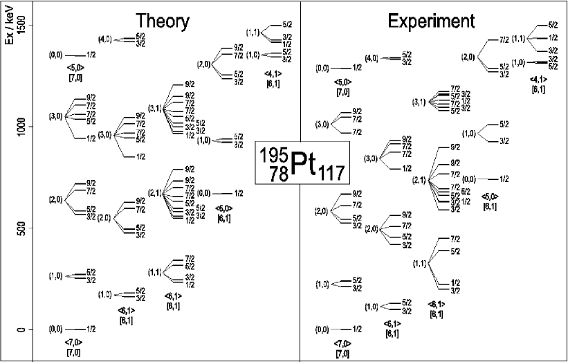
Figure 3: Comparison between the energy spectrum of the negative parity levels in the odd-neutron nucleus ¹⁹⁵Pt and that obtained for the $U(6/12)_{\nu}\otimes U(6/4)_{\pi}$ supersymmetry using Eq. (100) with $\alpha=52.5$, $\beta=8.7$, $\gamma=-53.9$, $\delta=48.8$, $\epsilon=8.8$ and $\eta=4.5$ in keV.

5.3 Dynamical supersymmetries

Boson-fermion symmetries can further be extended by introducing the concept of supersymmetries [22], in which states in both even-even and odd-even nuclei are treated in a single framework. In the previous section, we have discussed the symmetry properties of a mixed system of boson and fermion degrees of freedom for a fixed number of bosons $N$ and one fermion $M=1$. The operators $B_{ij}$ and $A_{\mu\nu}$

$$B_{ij}=b_{i}^{\dagger}b_{j}~{},\hskip 28.45274ptA_{\mu\nu}=a_{\mu}^{\dagger}a_{\nu}~{},$$ (75)

which generate the Lie algebra of the symmetry group $U^{B}(6)\otimes U^{F}(\Omega)$ of the IBFM, can only change bosons into bosons and fermions into fermions. The number of bosons $N$ and the number of fermions $M$ are both conserved quantities. As explained in Section 2.6, in addition to $B_{ij}$ and $A_{\mu\nu}$, one can introduce operators that change a boson into a fermion and vice versa

$$F_{i\mu}=b_{i}^{\dagger}a_{\mu}~{},\hskip 28.45274ptG_{\mu i}=a_{\mu}^{\dagger}b_{i}~{}.$$ (76)

The enlarged set of operators $B_{ij}$, $A_{\mu\nu}$, $F_{i\mu}$ and $G_{\mu i}$ forms a closed (super)algebra which consists of both commutation and anticommutation relations

$$\left[B_{ij},B_{kl}\right] = B_{il}\delta_{jk}-B_{kj}\delta_{il}~{},$$

$$\left[A_{\mu\nu},A_{\rho\sigma}\right] = A_{\mu\sigma}\delta_{\nu\rho}-A_{\rho\nu}\delta_{\mu\sigma}~{},$$

$$\left[B_{ij},A_{\mu\nu}\right] = 0~{},$$

$$\left[B_{ij},F_{k\mu}\right] = F_{i\mu}\delta_{jk}~{},$$

$$\left[G_{\mu i},B_{kl}\right] = G_{\mu l}\delta_{ik}~{},$$

$$\left[F_{i\mu},A_{\rho\sigma}\right] = F_{i\sigma}\delta_{\mu\rho}~{},$$

$$\left[A_{\mu\nu},G_{\rho i}\right] = G_{\mu i}\delta_{\nu\rho}~{},$$

$$\left\{F_{i\mu},G_{\nu j}\right\} = B_{ij}\delta_{\mu\nu}+A_{\nu\mu}\delta_{ij}~{},$$

$$\left\{F_{i\mu},F_{j\nu}\right\} = 0~{},$$

$$\left\{G_{\mu i},G_{\nu j}\right\} = 0~{}.$$ (77)

This algebra can be identified with that of the graded Lie group $U(6/\Omega)$. It provides an elegant scheme in which the IBM and IBFM can be unified into a single framework [22]

$$U(6/\Omega)\supset U^{B}(6)\otimes U^{F}(\Omega)~{}.$$ (78)

In this supersymmetric framework, even-even and odd-mass nuclei form the members of a supermultiplet which is characterized by ${\cal N}=N+M$, i.e. the total number of bosons and fermions. Supersymmetry thus distinguishes itself from “normal” symmetries in that it includes, in addition to transformations among fermions and among bosons, also transformations that change a boson into a fermion and vice versa.

$$\begin{array}[]{lcccccc}\hline\cr&&&&&&\\ \mbox{Model}&&\mbox{Generators}&&\mbox{Invariant}&&\mbox{Symmetry}\\ &&&&&&\\ \hline\cr&&&&&&\\ \mbox{IBM}&&b^{\dagger}_{i}b_{j}&&N&&\mbox{U(6)}\\ &&&&&&\\ \mbox{IBFM}&&b^{\dagger}_{i}b_{j}~{},\;a^{\dagger}_{\mu}a_{\nu}&&N,M&&\mbox{U(6)}\otimes\mbox{U($\Omega$)}\\ &&&&&&\\ \mbox{n-SUSY}&&b^{\dagger}_{i}b_{j}~{},\;a^{\dagger}_{\mu}a_{\nu}~{},\;b^{\dagger}_{i}a_{\mu}~{},\;a^{\dagger}_{\mu}b_{i}&&{\cal N}&&\mbox{U(6/$\Omega$)}\\ &&&&&&\\ \hline\cr\end{array}$$ (89)

The Os-Ir-Pt-Au mass region provides ample experimental evidence for the occurrence of dynamical (super)symmetries in nuclei. The even-even nuclei ^194,196Pt are the standard examples of the $SO(6)$ limit of the IBM [33] and the odd proton, in first approximation, occupies the single-particle level $2d_{3/2}$. In this special case, the boson and fermion groups can be combined into spinor groups, and the odd-proton nuclei ^191,193Ir and ^193,195Au were suggested as examples of the $Spin(6)$ limit [21, 30]. The appropriate extension to a supersymmetry is by means of the graded Lie group $U(6/4)$

$$U(6/4)\supset U^{B}(6)\otimes U^{F}(4) \supset SO^{B}(6)\otimes SU^{F}(4)$$ (90)

$$\supset Spin(6)\supset Spin(5)\supset Spin(3)\supset Spin(2)~{}.$$

The pairs of nuclei ¹⁹⁰Os - ¹⁹¹Ir, ¹⁹²Os - ¹⁹³Ir, ¹⁹²Pt - ¹⁹³Au and ¹⁹⁴Pt - ¹⁹⁵Au have been analyzed as examples of a $U(6/4)$ supersymmetry [22].

Another example of a dynamical supersymmetry in this mass region is that of the Pt nuclei. The even-even isotopes are well described by the $SO(6)$ limit of the IBM and the odd neutron mainly occupies the negative parity orbits $3p_{1/2}$, $3p_{3/2}$ and $3f_{5/2}$. In this case, the graded Lie group is $U(6/12)$

$$U(6/12)\supset U^{B}(6)\otimes U^{F}(12) \supset U^{B}(6)\otimes U^{F}(6)\otimes U^{F}(2)$$ (91)

$$\supset U^{BF}(6)\otimes U^{F}(2)$$

$$\supset SO^{BF}(6)\otimes U^{F}(2)$$

$$\supset SO^{BF}(5)\otimes U^{F}(2)$$

$$\supset SO^{BF}(3)\otimes SU^{F}(2)$$

$$\supset SU(2)~{}.$$

The odd-neutron nucleus ¹⁹⁵Pt, together with ¹⁹⁴Pt, were studied as an example of a $U(6/12)$ supersymmetry [23, 31, 32].

5.4 Dynamical neutron-proton supersymmetries

As we have seen in the previous section, the mass region $A\sim 190$ has been a rich source of possible empirical evidence for the existence of (super)symmetries in nuclei. The pairs of nuclei ¹⁹⁰Os - ¹⁹¹Ir, ¹⁹²Os - ¹⁹³Ir, ¹⁹²Pt - ¹⁹³Au and ¹⁹⁴Pt - ¹⁹⁵Au have been analyzed as examples of a $U(6/4)$ supersymmetry [22], and the nuclei ¹⁹⁴Pt - ¹⁹⁵Pt as an example of a $U(6/12)$ supersymmetry [23]. These ideas were later extended to the case where neutron and proton bosons are distinguished [28], predicting in this way a correlation among quartets of nuclei, consisting of an even-even, an odd-proton, an odd-neutron and an odd-odd nucleus. The best experimental example of such a quartet with $U(6/12)_{\nu}\otimes U(6/4)_{\pi}$ supersymmetry is provided by the nuclei ¹⁹⁴Pt, ¹⁹⁵Au, ¹⁹⁵Pt and ¹⁹⁶Au.

$$\begin{array}[]{ccccc}&{}^{194}_{78}\mbox{Pt}_{116}&\leftrightarrow&{}^{195}_{78}\mbox{Pt}_{117}&\\ &&&&\\ &\updownarrow&&\updownarrow&\\ &&&&\\ &{}^{195}_{79}\mbox{Au}_{116}&\hskip 28.45274pt\leftrightarrow&{}^{196}_{79}\mbox{Au}_{117}&\\ \end{array}$$ (97)

The number of bosons and fermions are related to the number of valence nucleons, i.e. the number of protons and neutrons outside the closed shells. The relevant closed shells are $Z=82$ for protons and $N=126$ for neutrons. For the even-even nucleus ${}^{194}_{78}\mbox{Pt}_{116}$ the number of bosons are $N_{\pi}=(82-78)/2=2$ and $N_{\nu}=(126-116)/2=5$. There are no unpaired nucleons $M_{\pi}=M_{\nu}=0$. For the odd-neutron nucleus ${}^{195}_{78}\mbox{Pt}_{117}$ there are 9 valence neutrons which leads to $N_{\nu}=4$ neutron bosons and $M_{\nu}=1$ unpaired neutron. The ${}_{79}\mbox{Au}$ isotopes have 3 valence protons which are divided over $N_{\pi}=1$ proton boson and $M_{\pi}=1$ unpaired proton. This supersymmetric quartet of nuclei is characterized by ${\cal N}_{\pi}=N_{\pi}+M_{\pi}=2$ and ${\cal N}_{\nu}=N_{\nu}+M_{\nu}=5$. The number of bosons and fermions are summarized in Table 1.

Table 1: The number of bosons and fermions of a supersymmetric quartet of nuclei.

Nucleus	$N_{\pi}$	$M_{\pi}$	$N_{\nu}$	$M_{\nu}$
${}^{194}_{78}\mbox{Pt}_{116}$	2	0	5	0
${}^{195}_{78}\mbox{Pt}_{117}$	2	0	4	1
${}^{195}_{79}\mbox{Au}_{116}$	1	1	5	0
${}^{196}_{79}\mbox{Au}_{117}$	1	1	4	1

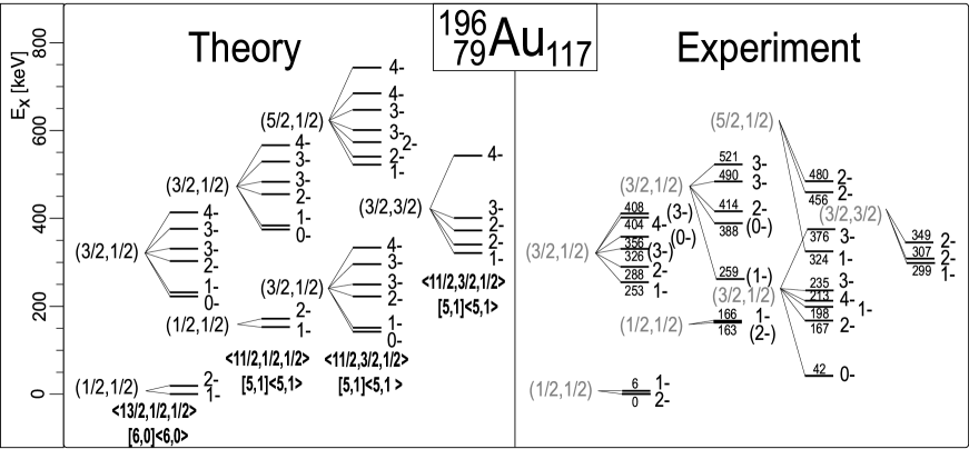
Figure 4: As Fig. 3, but for the negative parity levels in the odd-odd nucleus ¹⁹⁶Au.

In previous sections, we have used a schematic Hamiltonian consisting only of a quadrupole-quadrupole interaction to discuss the different dynamical symmetries. In general, a dynamical (super)symmetry arises whenever the Hamiltonian is expressed in terms of the Casimir invariants of the subgroups in a group chain. The relevant subgroup chain of $U(6/12)_{\nu}\otimes U(6/4)_{\pi}$ for the Pt and Au nuclei is given by [28]

$$U(6/12)_{\nu}\otimes U(6/4)_{\pi} \supset U^{B_{\nu}}(6)\otimes U^{F_{\nu}}(12)\otimes U^{B_{\pi}}(6)\otimes U^{F_{\pi}}(4)$$ (98)

$$\supset U^{B}(6)\otimes U^{F_{\nu}}(6)\otimes U^{F_{\nu}}(2)\otimes U^{F_{\pi}}(4)$$

$$\supset U^{BF_{\nu}}(6)\otimes U^{F_{\nu}}(2)\otimes U^{F_{\pi}}(4)$$

$$\supset SO^{BF_{\nu}}(6)\otimes U^{F_{\nu}}(2)\otimes SU^{F_{\pi}}(4)$$

$$\supset Spin(6)\otimes U^{F_{\nu}}(2)$$

$$\supset Spin(5)\otimes U^{F_{\nu}}(2)$$

$$\supset Spin(3)\otimes SU^{F_{\nu}}(2)$$

$$\supset SU(2)~{}.$$

In this case, the Hamiltonian

$$H = \alpha\,\hat{\cal C}_{2U^{BF_{\nu}}(6)}+\beta\,\hat{\cal C}_{2SO^{BF_{\nu}}(6)}+\gamma\,\hat{\cal C}_{2Spin(6)}$$ (99)

$$+\delta\,\hat{\cal C}_{2Spin(5)}+\epsilon\,\hat{\cal C}_{2Spin(3)}+\eta\,\hat{\cal C}_{2SU(2)}~{},$$

describes simultaneously the excitation spectra of the quartet of nuclei. Here we have neglected terms that only contribute to binding energies. The energy spectrum is given by the eigenvalues of the Casimir operators

$$E = \alpha\,\left[N_{1}(N_{1}+5)+N_{2}(N_{2}+3)+N_{3}(N_{3}+1)\right]$$ (100)

$$+\beta\,\left[\Sigma_{1}(\Sigma_{1}+4)+\Sigma_{2}(\Sigma_{2}+2)+\Sigma_{3}^{2}\right]$$

$$+\gamma\,\left[\sigma_{1}(\sigma_{1}+4)+\sigma_{2}(\sigma_{2}+2)+\sigma_{3}^{2}\right]$$

$$+\delta\,\left[\tau_{1}(\tau_{1}+3)+\tau_{2}(\tau_{2}+1)\right]+\epsilon\,J(J+1)+\eta\,L(L+1)~{}.$$

The coefficients $\alpha$, $\beta$, $\gamma$, $\delta$, $\epsilon$ and $\eta$ have been determined in a simultaneous fit of the excitation energies of the four nuclei of Eq. (97) [27].

The supersymmetric classification of nuclear levels in the Pt and Au isotopes has been re-examined by taking advantage of the significant improvements in experimental capabilities developed in the last decade. High resolution transfer experiments with protons and polarized deuterons have strengthened the evidence for the existence of supersymmetry in atomic nuclei. The experiments include high resolution transfer experiments to ¹⁹⁶Au at TU/LMU München [25, 26], and in-beam gamma ray and conversion electron spectroscopy following the reactions ¹⁹⁶Pt$(d,2n)$ and ¹⁹⁶Pt$(p,n)$ at the cyclotrons of the PSI and Bonn [27]. These studies have achieved an improved classification of states in ¹⁹⁵Pt and ¹⁹⁶Au which give further support to the original ideas [21, 23, 28] and extend and refine previous experimental work in this research area.

In dynamical (super)symmetries closed expressions can be derived for energies, as well as selection rules and intensities for electromagnetic transitions and transfer reactions. Recent work in this area concerns a study of one- and two-nucleon transfer reactions:

• As a consequence of the supersymmetry, explicit correlations were found between the spectroscopic factors of the one-proton reactions between n-SUSY partners ${}^{194}\mbox{Pt}\leftrightarrow^{195}\mbox{Au}$ and ${}^{195}\mbox{Pt}\leftrightarrow^{196}\mbox{Au}$ [34] which can be tested experimentally.

• The spectroscopic stengths of two-nucleon transfer reactions constitute a stringent test for two-nucleon correlations in the nuclear wave functions. A study in the framework of nuclear supersymmetry led to a set of closed analytic expressions for ratios of spectroscopic factors. Since these ratios are parameter independent they provide a direct test of the wave functions. A comparison between the recently measured ${}^{198}\mbox{Hg}(\vec{d},\alpha)^{196}\mbox{Au}$ reaction [35] and the predictions of the nuclear quartet supersymmetry [36] lends further support to the validity of supersymmetry in nuclear physics.

6 Prehispanic supersymmetry

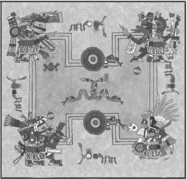
Figure 5: Prehispanic supersymmetry

Fig. 5 shows an artistic interpretation of supersymmetry in physics. This figure is part of the design of the poster of the XXXV Latin-American School of Physics. Supersymmetries in Physics and its Applications (ELAF 2004) by Renato Lemus which is inspired by the concept of supersymmetry as used in nuclear and particle physics and the ‘Juego de Pelota’, the ritual game of prehispanic cultures of Mexico. The four players on the ballcourt are aztec gods which represent the nuclei of a supersymmetric quartet. Each one of the gods represents a nucleus, on the top left Tezcatlipoca: the even-even nucleus ¹⁹⁴Pt, top right Quetzalcóatl: the odd-even nucleus ¹⁹⁵Pt, bottom left Camaxtle: the even-odd nucleus ¹⁹⁵Au, and finally Huitzilopochtli: the odd-odd nucleus ¹⁹⁶Au. The association between the gods and the nuclei is made via the number and the color of the balls that each one of the players carry. Each player carries 7 balls. The green and blue balls correspond to the neutron and proton bosons, whereas the yellow and red ones correspond to neutrons and protons, respectively. The one-nucleon transfer operators that induce the supersymmetric transformation between different nuclei, are represented by red coral snakes (‘coralillos’). The snakes that create a particle carry a ball in their mouth whose color indicates the type of particle. On the other hand, the snakes that annihilate a particle carry the corresponding ball soaking with blood that seems to split their body. Both types of snakes we see in segmented form, in representation of the quantization of energy. In the world of the ancient Mexico both living and dead creatures form a coherent unity and harmonize in the same plane of importance. This is reflected in the eyes that are included in all components of a graphical representation. For this reason, the balls associated with the creation and annihilation of particles have eyes.

The central figure in the ball court consists of two intertwined snakes, a coral snake and a rattle snake. They represent another aspect of supersymmetry as it is used in particle physics, in which each particle has its supersymmetric counterpart. The reason that this is symbolized by snakes is their property to change skins. Thus, a change of skin of two apparently different snakes suggests the transformation between bosons and fermions. The same two snakes make their appearance on the circular stone rings, the ‘score board’ of the aztec ball game. In the ball court one finds, at the feet of Tezcatlipoca the symbol Ollin, movement, which represents the uncertainty principle. Similarly, we see a heart in the upper right and the lower left part. The hearts have two meanings. On the one hand they characterize the ritual aspect of the ancient game ‘Juego de Pelota’ and, on the other hand, they represent the ‘road with a heart’, which science could follow. Finally, next to Huitzilopochtli there is a skull to remind us of the fleeting nature of our existence.

More information can be found in the proceedings of the ELAF 2004 [37].

7 Summary and conclusions

The concept of symmetry has played a very important role in physics, especially in the 20th century with the development of quantum mechanics and quantum field theory. The applications involve among other geometric symmetries, permutation symmetries, space-time symmetries, gauge symmetries and dynamical symmetries. In these lecture notes, I have concentrated mainly on the latter. The basic idea of dynamical symmetries is that of finding order, regularity and simple patterns in complex many-body systems. The examples discussed in these notes include isospin and flavor symmetry and nuclear supersymmetry.

Dynamical symmetries not only provide classification schemes for finite quantal systems and simple benchmarks against which the experimental data can be interpreted in a clear and transparent manner, but also led to important predictions that have been verified later experimentally, such as the $\Omega^{-}$ baryon as the missing member of the baryon decuplet, the nucleus ¹⁹⁶Pt as an example of the $SO(6)$ limit of the IBM and the odd-odd nucleus ¹⁹⁶Au whose spectroscopic properties had been predicted as a consequence of nuclear supersymmetry almost 15 years before they were measured.

The interplay between theory and experiment is reflected in the combination of the Platonic ideal of symmetry with the more down-to-earth Aristotelic ability to recognize complex patterns in Nature.

Figure 6: Detail of “The School of Athens” (Plato on the left and Aristoteles on the right), by Rafael.

References

- [1] See e.g. MacTutor History of Mathematics archive, School of Mathematics and Statistics, University of St. Andrews, Scotland http://www-history.mcs.st-andrews.ac.uk/history
- [2] F. Iachello, Nucl. Phys. A 751, 329c (2005).
- [3] W. Pauli, Z. Physik 36, 336 (1926).
- [4] P. Van Isacker, Rep. Prog. Phys. 62, 1661 (1999); Nucl. Phys. A 704, 232c (2002).
- [5] A. Frank, J. Barea and R. Bijker, in The Hispalensis Lectures on Nuclear Physics, Vol. 2, Eds. J.M. Arias and M. Lozano, Lecture Notes in Physics 652 (2004), 285-324 [arXiv:nucl-th/0402058].
- [6] M. Hamermesh, Group Theory and its Applications to Physical Problems, (Addison Wesley, Reading, 1962 and Dover Publications, New York, 1989).
- [7] H.J. Lipkin, Lie Groups for Pedestrians, (North-Holland, Amsterdam, 1966 and Dover Publications, New York, 2002).
- [8] R. Gilmore, Lie Groups, Lie Algebras, and Some of Their Applications, (Wiley-Interscience, New York, 1974).
- [9] B.G. Wybourne, Classical Groups for Physicists, (Wiley-Interscience, New York, 1974).
- [10] J.P. Elliott and P.G. Dawber, Symmetry in Physics, (Oxford University Press, Oxford, 1979).
- [11] H. Georgi, Lie Algebras in Particle Physics: from Isospin to Unified Theories, (Addison Wesley, 1982)
- [12] Fl. Stancu, Group Theory in Subnuclear Physics, (Oxford University Press, Oxford, 1996)
- [13] E.L. Hill, Rev. Mod. Phys. 23, 253 (1951).
- [14] W. Heisenberg, Z. Phys. 77, 1 (1932).
- [15] A. Bohr and B.R. Mottelson, Nuclear Structure. II. Nuclear Deformations (Benjamin, New York, 1975).
- [16] M. Gell-Mann, Phys. Rev. 125, 1067 (1962).
- [17] S. Okubo, Progr. Theor. Phys. 27, 949 (1962).
- [18] M. Gell-Mann and Y. Ne’eman, The Eightfold Way, (Benjamin, New York, 1964).
- [19] F. Iachello and A. Arima, The Interacting Boson Model, (Cambridge University Press, Cambridge, 1987).
- [20] F. Iachello and P. Van Isacker, The Interacting Boson-Fermion Model (Cambridge University Press, Cambridge, 1991).
- [21] F. Iachello, Phys. Rev. Lett. 44, 772 (1980).
-
[22]
A.B. Balantekin, I. Bars and F. Iachello,
Phys. Rev. Lett. 47, 19 (1981);
A.B. Balantekin, I. Bars and F. Iachello, Nucl. Phys. A 370, 284 (1981). - [23] A.B. Balantekin, I. Bars, R. Bijker and F. Iachello, Phys. Rev. C 27, 1761 (1983).
- [24] R. Bijker, Ph.D. Thesis, University of Groningen (1984).
- [25] A. Metz, J. Jolie, G. Graw, R. Hertenberger, J. Gröger, C. Günther, N. Warr and Y. Eisermann, Phys. Rev. Lett. 83, 1542 (1999).
- [26] A. Metz, Y. Eisermann, A. Gollwitzer, R. Hertenberger, B.D. Valnion, G. Graw and J. Jolie, Phys. Rev. C 61, 064313 (2000).
- [27] J. Gröger, J. Jolie, R. Krücken, C.W. Beausang, M. Caprio, R.F. Casten, J. Cederkall, J.R. Cooper, F. Corminboeuf, L. Genilloud, G. Graw, C. Günther, M. de Huu, A.I. Levon, A. Metz, J.R. Novak, N. Warr and T. Wendel, Phys. Rev. C 62, 064304 (2000).
- [28] P. Van Isacker, J. Jolie, K. Heyde and A. Frank, Phys. Rev. Lett. 54, 653 (1985).
- [29] J.P. Elliott, Proc. Roy. Soc. A 245, 128 (1958); ibid. 245, 562 (1958).
- [30] F. Iachello and S. Kuyucak, Ann. Phys. (N.Y.) 136, 19 (1981).
- [31] R. Bijker and F. Iachello, Ann. Phys. (N.Y.) 161, 360 (1985).
-
[32]
H.Z. Sun, A. Frank and P. Van Isacker,
Phys. Rev. C 27, 2430 (1983);
H.Z. Sun, A. Frank and P. Van Isacker, Ann. Phys. (N.Y.) 157, 183 (1984). -
[33]
J.A. Cizewski, R.F. Casten, G.J. Smith, M.L. Stelts, W.R. Kane,
H.G. Börner and W.F. Davidson,
Phys. Rev. Lett. 40, 167 (1978);
A. Arima and F. Iachello, Phys. Rev. Lett. 40, 385 (1978). - [34] J. Barea, R. Bijker and A. Frank, J. Phys. A: Math. Gen. 37, 10251 (2004).
- [35] H.-F. Wirth, G. Graw, S. Christen, Y. Eisermann, A. Gollwitzer, R. Hertenberger, J. Jolie, A. Metz, O. Möller, D. Tonev and B.D. Valnion, Phys. Rev. C 70, 014610 (2004).
- [36] J. Barea, R. Bijker and A. Frank, Phys. Rev. Lett. 94, 152501 (2005).
- [37] R. Lemus, in Latin-American School of Physics XXXV ELAF. Supersymmetries in Physics and its Applications, Eds. R. Bijker et al., AIP Conference Proceedings 744 (2005), xi-xvi.