Spin observables in ${\bar{\mathrm{p}}\mathrm{p}\to\overline{\Lambda}\Lambda}$
and density-matrix constraints ${}^{\;,}$

Abstract

The positivity conditions of the spin density matrix constrain the spin observables of the reaction ${\bar{\mathrm{p}}\mathrm{p}\to\overline{\Lambda}\Lambda}$, leading to model-independent, non-trivial inequalities. The formalism is briefly presented and examples of inequalities are provided.

1 Introduction

The strangeness-exchange reaction ${\bar{\mathrm{p}}\mathrm{p}\to\overline{\Lambda}\Lambda}$ has been studied at low energy by the PS185 collaboration with the antiproton beam of the LEAR facility at CERN. Experimental data on spin observables with a transversely-polarized proton target have been published Bassalleck:2002sd ; Pas2001 . This contribution is devoted to the inequalities relating two or three spin observables, which can be derived either empirically or by imposing positivity conditions to the density matrix.

2 Empirical approach

In Ref.Elchikh:1999ir , a number of inequalities among the spin observables has been written down. The method consists in generating randomly the real and imaginary parts of the complex amplitudes, computing the various observables and plotting one observable against another. Each observable $\mathcal{O}_{i}$ is typically normalized as $-1\leq\mathcal{O}_{i}\leq+1$. If a pair of randomly-generated observables, $\{\mathcal{O}_{i},\mathcal{O}_{j}\}$, covers the whole square $[-1,+1]^{2}$, there is no correlation between these observables. Very often, however, the domain is restricted to a disk or a triangle inner to the square, revealing that there exists an inequality of the type $\mathcal{O}_{i}^{2}+\mathcal{O}_{j}^{2}\leq~{}1$, or $4\mathcal{O}_{j}^{2}\leq(\mathcal{O}_{i}+1)^{2}$, which can be derived by inspecting the explicit expressions of these observables.

This method can be extended to the case of a triplet of observables. Examples of such plots are given in the figure. In the third plot, an inequality $\mathcal{O}_{1}^{2}+\mathcal{O}_{2}^{2}+\mathcal{O}_{3}^{2}\leq 1$ is observed, with obvious consequences for the projections,such as $\mathcal{O}_{1}^{2}+\mathcal{O}_{2}^{2}\leq 1$. In the fourth plot, however, the $\{\mathcal{O}_{1},\mathcal{O}_{2},\mathcal{O}_{3}\}$ domain is limited by a cubic surface, but there is no restriction on each $\{\mathcal{O}_{i},\mathcal{O}_{j}\}$ pair.

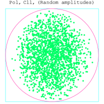
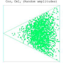
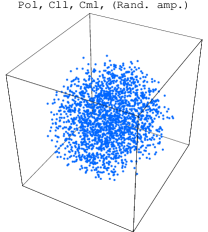
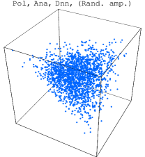
Figure 1: Simulation of observables by randomly generated amplitudes: from left to right, $P$ vs. $C_{ll}$, $C_{nn}$ vs. $C_{ml}$, $P$ vs. $C_{ll}$ and $C_{ml}$, and $P$ vs. $A$ and $D_{nn}$.

3 Explicit density matrix formalism

Let us now turn to the formalism of the spin-density matrix. Any diagonal element of the density matrix $\rho$ is positive, i.e., $\rho_{ii}\geq 0$. For any $2\times 2$ restriction, $\rho_{ii}.\rho_{jj}\geq\mid\rho_{ij}\mid^{2}$. This is sufficient for this survey. More general relations deduced from positivity are discussed in Ref.Richard:2003bu ; Artru:2004jx .

The density matrix for a polarized set of particles with spin 1/2 is

$$\rho_{p}=\frac{1}{2}(I+\boldsymbol{P}.\boldsymbol{\sigma})~{},$$ (1)

where $\boldsymbol{\sigma}=\{\sigma_{1},\sigma_{2},\sigma_{3}\}$ is made of the usual Pauli matrices, and $\boldsymbol{P}$ is the vector polarization. For the proton target, in our case, $\boldsymbol{P}$ is transverse to the unit-vector $\widehat{z}$ indicating the direction of the antiproton beam. In the ideal case of a 100% polarised target,

$$\boldsymbol{P}=\sin{\phi}\ \hat{x}+\cos{\phi}\ \hat{n}~{},$$ (2)

where $\hat{n}$ is normal to the scattering plane, and $\hat{x}=\hat{n}\times\hat{z}$. The spin-density matrix of the initial ${\bar{\mathrm{p}}\mathrm{p}}$ state is thus

$$\rho_{\bar{\mathrm{p}}\mathrm{p}}=\frac{1}{4}[I\otimes I+\sin{\phi}\ (I\otimes\widehat{x}.\overrightarrow{\sigma})+\cos{\phi}\ (I\otimes\widehat{n}.\overrightarrow{\sigma})]~{},$$ (3)

and we shall adopt the usual convention, see Ref.Elchikh:2004ex , that whilst the proton spin is projected on the $\{\hat{z},\hat{x},\hat{n}\}$, the antiproton one is writtten in the basis $\{-\hat{z},-\hat{x},-\hat{n}\}$. The explicit form is

$$\rho_{{\bar{\mathrm{p}}\mathrm{p}}}=\frac{1}{4}\sum\limits_{i=0,x,n}P_{i}(I\otimes\sigma_{i})=\frac{1}{4}\left(\begin{array}[]{llll}1&-ie^{-i\phi}&0&0\\ ie^{i\phi}&1&0&0\\ 0&0&1&-ie^{-i\phi}\\ 0&0&ie^{i\phi}&1\end{array}\right)~{},$$ (4)

where $P_{0}\equiv 1$, $\sigma_{0}\equiv I$ (the identity matrix). If $M$ is the transition matrix (amplitude) of the reaction ${\bar{\mathrm{p}}\mathrm{p}\to\overline{\Lambda}\Lambda}$, as written, e.g., in Elchikh:1999ir , the density matrix of the final state ${\overline{\Lambda}\Lambda}$ reads

$$\rho_{\overline{\Lambda}\Lambda}=M\rho_{\overline{p}p}M^{\dagger}=\frac{1}{4}\sum\limits_{i=0,x,n}P_{i}\ M\ (I\otimes\sigma_{i})\ M^{\dagger}~{}.$$ (5)

Using the Pauli matrices of $\overline{\Lambda}$ and $\Lambda$, respectively, it can be decomposed as

$$\rho_{\overline{\Lambda}\Lambda}=\frac{1}{4}I_{0}\sum\limits_{j,k=0,x,n,z}\left[\sum\limits_{i=0,x,n}P_{i}\ O_{ijk}\ (\sigma_{j}\otimes\sigma_{k})\right]~{},$$ (6)

this defining

• the differential cross section $I_{0}\equiv(1/4)\rm{Tr}(MM^{\dagger})$,

• the spin observables. $O_{ijk}\equiv\rm{Tr}[M\ (I\otimes\sigma_{i})\ M^{\dagger}\ (\sigma_{j}\otimes\sigma_{k}]/\rm{Tr}(MM^{\dagger})$.

More explicitly,

$$\rho_{\overline{\Lambda}\Lambda}(\phi)=\frac{1}{4}I_{0}(C_{0}+\cos{\phi}\ C_{n}+\sin{\phi}\ C_{x})~{},$$ (7)

where

$$C_{0}\equiv\sum\limits_{j,k}O_{0jk}\ (\sigma_{j}\otimes\sigma_{k})~{},\quad C_{x}\equiv\sum\limits_{j,k}O_{xjk}\ (\sigma_{j}\otimes\sigma_{k})~{},\quad C_{n}\equiv\sum\limits_{j,k}O_{njk}\ (\sigma_{j}\otimes\sigma_{k})~{},$$ (8)

The strong interaction responsible for the ${\bar{\mathrm{p}}\mathrm{p}\to\overline{\Lambda}\Lambda}$ reaction conserves many discrete symmetries such as parity and charge conjugation. Thus some observables vanish or are related to some others. It remains a set of only $21$ independent observables. For those of rank 1 or 2, $O_{ijk}$ is replaced by the more familiar notation: $P$ (polarization), $A$ (asymmetry), $C_{jk}$ (correlation), $D_{jk}$ (spin depolarization) and $K_{jk}$ (spin transfer), leading to

$$C_{0}=\left(\begin{array}[]{cccc}1-C_{zz}&-C_{xz}-iP_{n}&-C_{xz}-iP_{n}&-C_{nn}-C_{xx}\\ -C_{xz}+iP_{n}&1+C_{zz}&C_{nn}-C_{xx}&C_{xz}-iP_{n}\\ -C_{xz}+iP_{n}&C_{nn}-C_{xx}&1+C_{zz}&C_{xz}-iP_{n}\\ -C_{nn}-C_{xx}&C_{xz}+iP_{n}&C_{xz}+iP_{n}&1-C_{zz}\end{array}\right)~{},$$

$$C_{x}=\left(\begin{array}[]{cccc}-D_{xz}+K_{xz}&-iO_{xzn}-D_{xx}&K_{xx}+iO_{xnz}&i(O_{xnx}-O_{xxn})\\ -D_{xx}+iO_{xzn}&D_{xz}+K_{xz}&i(O_{xnx}+O_{xxn})&K_{xx}-iO_{xnz}\\ K_{xx}-iO_{xnz}&-i(O_{xnx}+O_{xxn})&-D_{xz}-K_{xz}&-D_{xx}+iO_{xzn}\\ i(O_{xxn}-O_{xnx})&K_{xx}+iO_{xnz}&-D_{xx}-iO_{xzn}&D_{xz}-K_{xz}\end{array}\right)~{},$$ (9)

$$C_{n}=\left(\begin{array}[]{cccc}A_{n}+O_{nxx}&-O_{nzx}-iD_{nn}&-O_{nxz}-iK_{nn}&-A_{n}-O_{nxx}\\ -O_{nzx}+iD_{nn}&A_{n}-O_{nxx}&A_{n}-O_{nxx}&O_{nxz}-iK_{nn}\\ -O_{nxz}+iK_{nn}&A_{n}-O_{nxx}&A_{n}-O_{nxx}&O_{nzx}-iD_{nn}\\ -A_{n}-O_{nxx}&O_{nxz}+iK_{nn}&O_{nzx}+iD_{nn}&A_{n}+O_{nxx}\end{array}\right)~{}.$$

The relation $\rho_{11}\rho_{22}\geq|\rho_{12}|^{2}$ gives

$$(1-C_{zz})(1+C_{zz})\geq\left|-C_{xz}-iP_{n}\right|^{2}~{},\quad\hbox{i.e.,}\quad C_{xz}^{2}+P_{n}^{2}+C_{zz}^{2}\leq 1~{},$$ (10)

which, of course, implies

$$C_{xz}^{2}+P_{n}^{2}\leq 1~{},\quad C_{zz}^{2}+P_{n}^{2}\leq 1~{},\quad C_{xz}^{2}+C_{zz}^{2}\leq 1~{}.$$ (11)

Similarly,

$$(1+C_{zz})^{2}\geq(P_{n}+C_{xz})^{2}~{}.$$ (12)

If the polarization of the proton target is introduced, the positivity of $\rho_{\overline{\Lambda}\Lambda}(0)$ and $\rho_{\overline{\Lambda}\Lambda}(\pi)$, which mixes the elements of the two blocks $C_{0}$ and $C_{n}$, induces

$$O_{nxx}^{2}+O_{nzx}^{2}+C_{xz}^{2}+P_{n}^{2}+D_{nn}^{2}+C_{zz}^{2}\leq 1+A_{n}^{2}~{}.$$ (13)

Here, with the use of the explicit expressions of the spin observables in terms of the complex parameters, it can be shown that

$$D_{nn}^{2}+C_{zz}^{2}+O_{nzx}^{2}\leq 1~{},$$ (14)

which leads to: $D_{nn}^{2}+O_{nzx}^{2}\leq 1$ and $C_{zz}^{2}+O_{nzx}^{2}\leq 1$ and the already-published Elchikh:1999ir ; Richard:1996bb inequality:

$$D_{nn}^{2}+C_{zz}^{2}\leq 1~{}.$$ (15)

4 Summary

Inequalities among spin observables can be derived either from the explicit expressions of these observables in terms of the amplitudes, or from the general properties of the spin density matrix. These inequalities provide model-independent test of the data on spin observables. Similar inequalities can be written down in the case of inclusive reactions or spin-dependent parton densities Artru:2004jx ; Soffer:2003qj . This will be the subject of a forthcoming review article AERST . The formalism of the spin density matrix is clearly more powerful, and it suggests a more physical interpretation of the inequalities, which can be read as the flow of quantum information from the initial to the final state.

References

• (1) B.Β Bassalleck et al. [PS185 collaboration], Phys.Β Rev.Β Lett.Β  89, 212302 (2002) [arXiv:nucl-ex/0206005].
• (2) K. Paschke, Carnegie Mellon University Thesis (2001), available at:
http://www-meg.phys.cmu.edu/~paschke/.
• (3) M.Β Elchikh and J.Β M.Β Richard, Phys.Β Rev.Β C 61, 035205 (2000) [arXiv:hep-ph/9905400].
• (4) J.Β M.Β Richard and X.Β Artru, Nucl.Β Instrum.Β Meth.Β B 214, 171 (2004) [arXiv:nucl-th/0304015] (Proc. LEAP2003 Conference, Yokohama, Japan, 2003).
• (5) X.Β Artru and J.Β M.Β Richard, Phys.Β Part.Β Nucl.Β  35 (2004) S126 [arXiv:hep-ph/0401234] (Proc. Xth Advanced Research Workshop on High Energy Spin Physics, 2003, Dubna).
• (6) M.Β Elchikh, Acta Phys.Β Polon.Β B 35, 2439 (2004).
• (7) J.Β M.Β Richard, Phys.Β Lett.Β B 369, 358 (1996) [arXiv:nucl-th/9601015].
• (8) J.Β Soffer, Phys.Β Rev.Β Lett.Β  91, 092005 (2003) [arXiv:hep-ph/0305222].
• (9) X. Artru, M. Elchikh, J.-M. Richard, J. Soffer and O.V. Teryaev, Phys. Rep. in preparation.