Representations in Density Dependent Hadronic Field Theory and compatibility with QCD sum-rules

Abstract

Different representations of an effective, covariant theory of the hadronic interaction are examined. For this purpose we have introduced nucleon-meson vertices parametrized in terms of scalar combinations of hadronic fields, extending the conceptual frame of the Density Dependent Hadronic Field Theory. Nuclear matter properties at zero temperature are examined in the Mean Field Approximation, including the equation of state, the Landau parameters, and collective modes. The treatment of isospin channels in terms of QCD sum rules inputs is outlined.

I Introduction

A generalized concept in present theoretical physics is that description of all physical phenomena should be derivable from first principles in a unified way. However, the bridge towards concrete applications requires elaborated procedures and judicious arguments. This is the case of Quantum Chromodynamics (QCD), which is the accepted theoretical model for the strong interactions. Despite the fact that it is perturbative in the high energy regime, the fundamental state of matter corresponds to the opposite limit, where confinement and the breakdown of symmetries make it mathematically intractable. Different effective models, such as Nambu- Jona Lasinio, Skyrme, bag-like, and chiral perturbation theory attempts to translate the main features of QCD into the hadronic phase. On the other hand, lattice simulations and QCD sum-rules share this aim, although using different methods.
QCD sum-rules is a ingenious procedure to reveal the foundations of certain hadronic properties. The method is based on the evaluation of correlation functions in terms of quarks and gluons degrees, then applying the operator product expansion it is possible to express it as combinations of perturbative contributions and condensates (non-perturbative). Finally this expansion is connected with the hadronic counterpart by means of a Borel transformation. The method was developed to study meson SHIFMAN as well as baryon IOFFE properties in vacuum, it was subsequently generalized to study finite density systems DRUKAREV0 ; DRUKAREV . These calculations provide a useful guide for some static properties of hadrons immersed in a dense medium, as concerning QCD symmetries and phenomenology. However, they are not able to take into account the dynamical aspects of hadronic matter, which may be achieved by inserting coherently these results into a theoretical model of hadronic interactions.
A similar situation was found in the study of nuclear structure, as the standard combination of microscopic potentials and the relativistic Dirac-Brueckner approximation for nuclear matter gives rise to reliable, density dependent, nucleon self-energies. Notwithstanding, this procedure was inadequate to treat finite nuclei due to unsurmountable mathematical difficulties. A feasible solution to this dilemma was proposed in TOKI ; HADDAD ; LENSKE ; TYPEL , by defining density dependent meson-nucleon vertices in terms of the self-energies obtained in Dirac-Brueckner calculations. The enlarged hadronic model keeps the mathematical versatility of the Quantum Hadrodynamic models WALECKA , but is equipped with couplings reflecting the properties of the nuclear environment. The structure of spherical nuclei, in the medium to heavy range, was studied within this framework using the Hartree approximation.
Further improvements, developed in LENSKE , replace the density dependence of the meson-nucleon vertices by an expansion in terms of in-medium nucleon condensates. This conceptual replacement restores the covariance and the thermodynamical consistency of the model, giving rise to the Density Dependent Hadronic Field Theory (DDHFT). It was recently appended by introducing momentum dependent vertices TYPEL2 , and a expansion of the vertices in terms of meson mean field values AGUIRRE .
The validity of the method is only justified a posteriori, and relies in the flexibility of hadronic field models to accommodate pieces of information provided by another field of research. The enlarged model yields a simpler and more intuitive description, instead of making involved calculations based on first principles interactions. A significative exemplification of this standpoint was given by the Brown-Rho scaling of hadronic masses. Taking into account the chiral and scale symmetries of QCD solely, an approximate scaling law for the in-medium hadronic masses was derived in BROWNRHO . This hypothesis was applied to describe heavy ion collision, reaching an excellent agreement with the experimental results for the low mass dilepton production rate BROWN .
Given a set of physically meaningful self-energies as input for DDHFT, there is room for a full family of hadronic models, according to the field parameterization assumed for the vertices. In principle, this may lead to different predictions for nuclear observables. This point has not been investigated yet, and it is the main purpose of the present work.
In a previous paper AGUIRRE , the author attempted to make use of the scheme outlined above to relate nuclear observables with QCD inspired results. For this purpose we took as input the nucleon self-energies in symmetric nuclear matter obtained in DRUKAREV by using QCD sum rules. However, Ref. AGUIRRE does not exhaust the physical description given there, as it covers isospin asymmetric nuclear matter also. So, we aim to complete our theoretical model including isospin degrees of freedom, based on the results presented in DRUKAREV .

We have organized this work presenting in the following section the general features of DDHFT, and particularly the meson parameterization of the hadronic vertices. In Section III we present and discuss the results for symmetric nuclear matter. A final summary is given in Section IV.

II Density Dependent Hadronic Field Theory

As mentioned above, DDHFT was designed to incorporate into the hadronic field formalism pieces of information produced by other theoretical frames. Strictly speaking, DDHFT takes as input the nucleon self-energies, which can be decomposed into iso-scalar and iso-vector components, each one containing Lorentz scalar and vector contributions: i. e. $\Sigma_{s}^{in}$, $\Sigma_{\mu}^{in}$, $\Sigma_{s}^{in\;a}$, $\Sigma_{\mu}^{in\;a}$, where the superscript $a$ distinguishes iso-vector quantities, and $a=1,2$ stands for proton and neutron respectively. For homogeneous nuclear matter in steady state, they can be parameterized as functions of continuous parameters, like baryonic current density $j_{\mu}$ and temperature, characterizing the macroscopic state of hadronic matter. In particular, there exists a reference frame where the spatial part of the baryonic current vanishes in the mean. In its former version $\Sigma^{in}$ was taken from relativistic Brueckner-Hartree-Fock calculations with one boson exchange potentials TOKI .

On the other hand, a lagrangian density is proposed in terms of meson fields $\sigma$, $\omega_{\mu}$ in the iso-scalar sector, and $\phi_{c}$, $\rho_{\mu}^{c}$ in the iso-vector one. The indices $c=1,2,3$ stand for the meson isospin projection

$${\mathcal{L}} = \bar{\Psi}(i\not\!\partial-M+\Gamma_{s}\,\sigma-\Gamma_{w}\not\!\omega+\Gamma_{f}^{c}\,\phi_{c}+\Gamma_{r}^{c}\,\not\!\rho_{c})\,\Psi$$

$$+ \frac{1}{2}(\partial_{\mu}\sigma\partial^{\mu}\sigma\,-m_{s}^{2}\sigma^{2})-\frac{1}{4}W_{\mu\nu}W^{\mu\nu}+\frac{1}{2}m_{w}^{2}\omega_{\mu}\omega^{\mu}$$

$$+ \frac{1}{2}(\partial_{\mu}\phi_{c}\partial^{\mu}\phi_{c}\,-m_{f}^{2}\phi^{2})-\frac{1}{4}R_{\mu\nu}^{c}R^{\mu\nu}_{c}+\frac{1}{2}m_{r}^{2}\rho_{\mu}^{c}\rho^{\mu}_{c},$$

where $W_{\mu\nu}=\partial_{\mu}\omega_{\nu}-\partial_{\nu}\omega_{\mu}$, $R_{\mu\nu}^{c}=\partial_{\mu}\rho_{\nu}^{c}-\partial_{\nu}\rho_{\mu}^{c}$ has been used, and $\Psi$ represents a isospinor. We have adopted the convention that repeated isospin indices must be summed. The isovector vertices $\Gamma^{c}$ take values over the space generated by the Pauli matrices $\tau$ and the identity. The masses have been fixed at the phenomenological values $M=940$ MeV, $m_{w}=783$ MeV, $m_{s}=550$ MeV, $m_{r}=770$ MeV, and $m_{f}=984$ MeV. The iso-scalar vertices are assumed to depend on the scalar combinations: $s_{1}=\sqrt{j_{\mu}j^{\mu}}$, $s_{2}=\bar{\Psi}\Psi$, $m_{1}=\sqrt{\omega_{\mu}\omega^{\mu}}$, and $m_{2}=\sigma$, whereas the isovector $\Gamma^{c}$ could depend linearly on $j_{c}=\bar{\Psi}\tau^{c}\Psi$, or $\phi_{c}$, and on the scalars $s_{3}=\sqrt{j_{\mu}^{c}j^{\mu}_{c}}$, $s_{4}=\sqrt{j_{c}j_{c}}$, $m_{3}=\sqrt{\rho_{\mu}^{c}\rho^{\mu}_{c}}$, and $m_{4}=\sqrt{\phi_{c}\phi_{c}}$. The baryonic and isospin current have been written as $j_{\mu}=\bar{\Psi}\gamma_{\mu}\Psi$ and $j_{\mu}^{c}=\bar{\Psi}\gamma_{\mu}\tau^{c}\Psi$, respectively. This is not the most general dependence, but it keeps a clear separation between isospin scalar and vector degrees of freedom. In Ref. LENSKE the dependence on $s_{1}$ or $s_{2}$ was presented and the case with only $s_{2}$ was explicitly studied; in AGUIRRE the meson dependence of the vertices was introduced within DDHFT, for symmetric nuclear matter.

The field equations obtained for this lagrangian density are

$$\left[(i\not\!\partial-M+\Gamma_{s}\,\sigma-\Gamma_{w}\not\!\omega)\delta_{AB}+\Gamma_{f\;AB}^{c}\,\phi_{c}+\Gamma_{r\;AB}^{c}\,\not\!\rho_{c}\right]\psi_{B}$$

$$\;\;\;+\bar{\Psi}\frac{\partial}{\partial\bar{\psi_{A}}}\left(\Gamma_{s}\sigma-\Gamma_{w}\not\!\omega+\Gamma_{f}^{c}\,\phi_{c}+\Gamma_{r}^{c}\,\not\!\rho_{c}\right)\Psi=0$$ (2)

$$\;\;\;\left(\square+m_{s}^{2}\right)\sigma=\bar{\Psi}\left[\Gamma_{s}+\left(\frac{\partial\Gamma_{s}}{\partial m_{2}}\sigma-\frac{\partial\Gamma_{w}}{\partial m_{2}}\not\!\omega\right)\right]\Psi$$ (3)

$$\;\;\;\partial_{\mu}W^{\mu\nu}+m_{w}^{2}\omega^{\nu}=\bar{\Psi}\left[\Gamma_{w}\gamma^{\nu}-\frac{\partial m_{1}}{\partial\omega_{\nu}}\left(\frac{\partial\Gamma_{s}}{\partial m_{1}}\sigma-\frac{\partial\Gamma_{w}}{\partial m_{1}}\not\!\omega\right)\right]\Psi.$$ (4)

$$\;\;\;\left(\square+m_{f}^{2}\right)\phi^{c}=\bar{\Psi}\left[\Gamma_{f}^{c}+\frac{\partial m_{4}}{\partial\phi_{c}}\left(\frac{\partial\Gamma_{f}^{a}}{\partial m_{4}}\phi_{a}+\frac{\partial\Gamma_{r}^{a}}{\partial m_{4}}\not\!\rho_{a}\right)\right]\Psi$$ (5)

$$\;\;\;\partial_{\mu}R^{\mu\nu}_{c}+m_{r}^{2}\rho^{\nu}_{c}=-\bar{\Psi}\left[\Gamma_{r\,c}\gamma^{\nu}+\frac{\partial m_{3}}{\partial\rho_{\nu}^{c}}\left(\frac{\partial\Gamma_{f}^{a}}{\partial m_{3}}\phi_{a}+\frac{\partial\Gamma_{r}^{a}}{\partial m_{3}}\not\!\rho_{a}\right)\right]\Psi,$$ (6)

where the isospin indices have been denoted as: $A,B=1,2$ for nucleons, and $a,c=1,2,3$ for mesons. In the first equation, the vertex derivatives must be interpreted as

$$\frac{\partial\Gamma}{\partial\bar{\psi_{A}}}=\sum_{1}^{4}\frac{\partial\Gamma}{\partial s_{k}}\frac{\partial s_{k}}{\partial\bar{\psi_{A}}}.$$

The mean field approximation (MFA) is suited to describe homogeneous matter. Within this scheme, meson fields are replaced by their uniform mean values and bilinear combinations of spinors are replaced by their expectation values. For homogeneous, isotropic nuclear matter in steady state, some simplifications arise in the meson mean values. For instance, their coordinate dependence can be neglected; the spatial components of the vectors $\omega_{\mu}$ and $\rho_{\mu}$ become null, and only the third component of the isovector mesons are non-zero, due to isospin conservation.
Therefore within MFA, Eqs. (2-6) reduce to

$$0=\left[(i\not\!\partial-M)\,\delta_{AB}+\Sigma_{s}^{AB}-\not\!\!\Sigma^{AB}\right]\psi_{B},$$ (7)

$$m_{s}^{2}\tilde{\sigma}=<\bar{\Psi}\,\Gamma_{s}\Psi>+<\bar{\Psi}\frac{\partial\Gamma_{s}}{\partial m_{2}}\Psi\,\sigma> - <\bar{\Psi}\frac{\partial\Gamma_{w}}{\partial m_{2}}\gamma_{\mu}\Psi\omega^{\mu}>;$$ (8)

$$g^{\nu}_{0}\;m_{w}^{2}\tilde{\omega}=<\bar{\Psi}\,\Gamma_{w}\gamma^{\nu}\Psi>-<\bar{\Psi}\,\frac{\partial\Gamma_{s}}{\partial m_{1}}\Psi\,\frac{\sigma\omega^{\nu}}{m_{1}}> + <\bar{\Psi}\frac{\partial\Gamma_{w}}{\partial m_{1}}\gamma_{\mu}\Psi\,\frac{\omega^{\nu}\omega^{\mu}}{m_{1}}>;$$ (9)

$$\delta_{3c}\;m_{f}^{2}\tilde{\phi}=<\bar{\Psi}\Gamma_{f}^{c}\Psi>+<\bar{\Psi}\frac{\partial\Gamma_{f}^{a}}{\partial m_{4}}\Psi\,\frac{\phi_{c}\phi_{a}}{m_{4}}> + <\bar{\Psi}\frac{\partial\Gamma_{r}^{a}}{\partial m_{4}}\gamma_{\mu}\Psi\frac{\phi_{c}}{m_{4}}\rho_{a}^{\mu}>;$$ (10)

$$-\delta_{3c}g^{\nu}_{0}m_{r}^{2}\tilde{\rho}=<\bar{\Psi}\Gamma_{r\,c}\gamma^{\nu}\Psi>+<\bar{\Psi}\frac{\partial\Gamma_{f}^{a}}{\partial m_{3}}\Psi\frac{\rho^{\nu}_{c}\phi_{a}}{m_{3}}> + <\bar{\Psi}\frac{\partial\Gamma_{r}^{a}}{\partial m_{3}}\gamma_{\mu}\Psi\frac{\rho^{\nu}_{c}\rho^{\mu}_{a}}{m_{3}}>;$$ (11)

where tildes over the meson symbols stand for their mean field values, and the two last terms within brackets in Eq. (7) can be regarded as the scalar and vector components of the nucleon self-energies:

$$\Sigma_{s}^{AB} = <\Gamma_{s}\sigma+\bar{\Psi}\Lambda_{2}\Psi>\delta_{AB}\,+<\Gamma_{f}^{c\,AB}\phi_{c}+\tau_{a}^{AB}\,\bar{\Psi}\Lambda_{4}\Psi\frac{\bar{\Psi}\tau_{a}\Psi}{s_{4}}>,$$ (12)

$$\Sigma_{\nu}^{AB} = <\Gamma_{w}\omega_{\nu}-\bar{\Psi}\Lambda_{1}\frac{j_{\nu}}{s_{1}}\Psi>\delta_{AB}\,-<\Gamma_{r\,c}^{AB}\rho_{\nu}^{c}+\tau_{a}^{AB}\,\bar{\Psi}\Lambda_{3}\Psi\frac{j_{\nu}^{a}}{s_{3}}>,$$ (13)

with $\Lambda_{k}=\partial\left(\Gamma_{s}\sigma-\Gamma_{w}\not\!\omega+\Gamma_{f}^{c}\phi_{c}+\Gamma_{r}^{c}\not\!\rho_{c}\right)/\partial s_{k}$ .

For the sake of concreteness, we have examined three possible parameterizations:

1. symmetric nuclear matter, with $\Gamma_{s}(s_{1})$, $\Gamma_{w}(s_{1})$;

2. symmetric nuclear matter, with $\Gamma_{s}(s_{2})$, $\Gamma_{w}(s_{1})$;

3. asymmetric nuclear matter, with $\Gamma_{s}(m_{2})$, $\Gamma_{w}(m_{1})$, $\Gamma_{f}^{c}(\phi^{c},m_{4})$, $\Gamma_{r}^{c}=\Gamma_{r}(\phi^{c},m_{3})$.

The first two cases are comparable to the instances presented in LENSKE as vector and scalar dependencies. The last case is a development of the preliminaries calculations of AGUIRRE , the field dependence of the isospin vertices have been chosen so as to adjust the QCD sum rules calculations of DRUKAREV .
These results are simplified within the assumptions (a-c) above, for the sake of completeness we consider separately each of these cases:

a) $$\,\Sigma_{s}=\Gamma_{s}\tilde{\sigma},\,\Sigma_{\nu}=g_{\nu 0}\left[\Gamma_{w}\tilde{\omega}+\frac{d\Gamma_{w}}{dn_{B}}\,\tilde{\omega}n_{B}-\frac{d\Gamma_{s}}{dn_{B}}\,\tilde{\sigma}n_{s}\right],$$

$$\tilde{\sigma}=\Gamma_{s}n_{s}/m_{s}^{2},\,\tilde{\omega}=\Gamma_{w}n_{B}/m_{v}^{2},$$

b) $$\,\Sigma_{s}=\tilde{\sigma}\left(\Gamma_{s}+\frac{d\Gamma_{s}}{dn_{s}}n_{s}\right),\,\Sigma_{\nu}=g_{\nu 0}\,\tilde{\omega}\left(\Gamma_{w}+\frac{d\Gamma_{w}}{dn_{B}}\,n_{B}\right),$$

$$\,\tilde{\sigma},\,\mbox{and}\;\tilde{\omega}\,\mbox{have the same expressions as in (a)},$$

c) $$\,\Sigma_{s}^{AB}=\Sigma_{s}^{isos}\delta_{AB}+\Sigma_{s}^{isov\,AB},\;\Sigma_{\nu}^{AB}=g_{\nu 0}\left(\Sigma_{v}^{isos}\delta_{AB}+\Sigma_{v}^{isov\,AB}\right),$$

$$\Sigma_{s}^{isos}=\Gamma_{s}\tilde{\sigma},\;\Sigma_{s}^{isov\,AB}=\Gamma^{3\,AB}_{f}\tilde{\phi},\;\Sigma_{v}^{isos}=\Gamma_{w}\tilde{\omega},\;\Sigma_{v}^{isov\,AB}=-\Gamma_{r}^{3\,AB}\tilde{\rho},$$

$$m_{s}^{2}\tilde{\sigma}=\frac{d\Sigma_{s}^{isos}}{d\tilde{\sigma}}n_{s},\;m_{w}^{2}\tilde{\omega}=\frac{d\Sigma_{v}^{isos}}{d\tilde{\omega}}n_{B},$$

$$m_{f}^{2}\tilde{\phi}=<\bar{\Psi}\frac{d\Sigma_{s}^{isov}}{d\tilde{\phi}}\Psi>-<\bar{\Psi}\frac{d\Sigma_{v}^{isov}}{d\tilde{\phi}}\gamma_{0}\Psi>,\;m_{r}^{2}\tilde{\rho}=<\bar{\Psi}\frac{d\Sigma_{v}^{isov}}{d\tilde{\rho}}\gamma_{0}\Psi>.$$

Obtaining the equations listed above, we have used the Wick theorem and the Hartree approximation, therefore contractions of fields belonging to different full contracted terms (both in Lorentz and isospin indices) have been neglected. This approach allowed us to extract the vertices $\Gamma$ and its derivatives from the expectation values, and to express the mean value of products of more than two fermion fields as product of baryonic densities and currents. Finally, we have adopted the reference frame of static matter, therefore we have $<j_{\mu}>=n_{B}\,g_{\mu 0}$, $<j_{\mu}^{c}>=(n_{B}^{(1)}-n_{B}^{(2)})\,g_{\mu 0}\delta_{3c}$, with $n_{B}^{A}=<\bar{\psi}_{A}\gamma_{0}\psi_{A}>$ the number of neutrons or protons per unit volume, for $A=2,1$ respectively, and $n_{B}=n_{B}^{(1)}+n_{B}^{(2)}$ the baryonic number density. Furthermore we have introduced the simplifying notation $n_{s}^{(A)}=<\bar{\psi}_{A}\psi_{A}>$, $n_{s}=<\bar{\Psi}\Psi>$, $\Gamma=<\Gamma>$, $s_{1}=n_{B}$, $s_{2}=n_{s}$, $s_{3}=\mid n_{B}^{(1)}-n_{B}^{(2)}\mid$, $s_{4}=\mid n_{s}^{(1)}-n_{s}^{(2)}\mid$, $m_{1}=\tilde{\omega}$, $m_{2}=\tilde{\sigma}$, $m_{3}=\tilde{\rho}$, and $m_{4}=\tilde{\phi}$.

Cases (a) and (b) yield meson equations resembling those of the Walecka model WALECKA , and nucleon self-energies with the rearrangement contributions added. In the instance (c) the self-energies have the same structure as in QHD-I, but the source term of the meson equations are modified. With respect to the isovector meson field equations, it must be noted that $<\bar{\Psi}\tau_{c}\Psi>=0$ for $c=1,2$ as isospin is a conserved charge. In order to give explicit expressions for the corresponding vertices, we follow the parameterization of DRUKAREV :

$$\Sigma_{k}^{AA\,(in)}=\frac{\alpha_{k}+I_{3}^{A}\beta_{k}t}{\lambda+n_{0}/n_{B}+I_{3}^{A}\,\alpha t},\;\;k=s,v$$ (17)

with $I_{3}^{A}=1(-1)$, for protons (neutrons), $n_{0}=0.17fm^{-3}$, $t=(n_{B}^{(2)}-n_{B}^{(1)})/n_{B}$, the remaining coefficients can be expressed in terms of the quantities used in Ref. DRUKAREV as $\lambda=C_{v}^{q}v_{N}+C_{g}^{q}g_{N}+C_{u1}^{q}+C_{\omega}^{q}A_{4q}^{q0}$, $\alpha=C_{u2}^{q}+C_{\omega}^{q}A_{4q}^{q1}$, $\alpha_{s}=M\lambda-C_{k}^{I}\kappa_{N}-C_{\omega}^{I}A_{4q}^{I0}$, $\beta_{s}=M\alpha-(C_{\zeta}^{I}\zeta_{N}+C_{\omega}^{I}A_{4q}^{I1})$, $\alpha_{v}=-(C_{v}^{p}v_{N}+MC_{u1}^{p}+MC_{\omega}^{p}A_{4q}^{p0}$), $\beta_{v}=-(C_{v-}^{p}v_{N}^{-}+MC_{u2}^{p}+MC_{\omega}^{p}A_{4q}^{p0})$, which were obtained in DRUKAREV , by averaging over the Borel mass. For the sake of completeness we give here the numerical values $v_{N}=3$, $v_{N}^{-}=1$, $g_{N}=-8M/9$, $\kappa_{N}=8$, $\zeta_{N}=0.54$, $C_{\kappa}^{I}=-0.042$ GeV; $C_{\zeta}^{I}=-0.042$ GeV; $C_{g}^{q}=0.011/GeV$; $C_{v-}^{p}=-0.068$ GeV; $C_{\omega}^{k}=-0.067,-0.095,-0.070$ GeV, $A_{4q}^{0k}=1.90,-0.57,-0.11$, and $A_{4q}^{1k}=-0.92,0.09,-0.21$ for $k=I,p$ and $q$ respectively; $C_{v}^{k}=-0.062,-0.090$, $C_{u1}^{k}=-0.074,0.094$, and $C_{u2}^{k}=0.008,-0.02$ for $k=q$ and $p$ respectively.
From Eq. (17), we can extract isoscalar and isovector contributions, i.e. we consider the splitting $\Sigma_{k}^{AA\,(in)}=\Sigma_{k}^{isos\,(in)}+\Sigma_{k\,A}^{isov\,(in)}$, with

$$\Sigma_{k}^{isos\,(in)}=\frac{\alpha_{k}n_{B}}{n_{0}+\lambda n_{B}},\;\;\Sigma_{k\,A}^{isov\,(in)}=I_{3}^{A}t\frac{\beta_{k}-\alpha^{\prime}_{k}\alpha n_{B}}{\lambda+n_{0}/n_{B}+I_{3}^{A}\alpha t},$$ (18)

with $\alpha^{\prime}_{k}=\alpha_{k}/(n_{0}+\lambda n_{B})$.
A choice of the isovector interaction in Eq. (II), which is coherent with these results is

$$\mathcal{L}_{iso}=\bar{\Psi}\tau^{c}\frac{G_{r}\not\!\rho_{c}+G_{f}\phi_{c}}{1+g\,\tau_{a}\phi^{a}}\Psi,$$

where $G_{r}$ is assumed to depend only on $m_{3}$, whereas $G_{f}$ and $g$ are considered as functions of $m_{4}$ only. The following vertices are deduced from it

$$\Gamma_{r}^{c}=\frac{G_{r}\tau^{c}(1-g\tau_{a}\phi^{a})}{1-g^{2}\phi^{2}},\;\;\Gamma_{f}^{c}=\frac{G_{f}\tau^{c}(1-g\tau_{a}\phi^{a})}{1-g^{2}\phi^{2}}.$$

In the MFA, they give rise to the following contributions to the nucleon self-energies

$$\Sigma_{v}^{isov\,AB}=-\delta_{AB}\frac{I_{3}^{A}G_{r}\tilde{\rho}}{1+I_{3}^{A}\,g\tilde{\phi}},\;\;\Sigma_{s}^{isov\,AB}=\delta_{AB}\frac{I_{3}^{A}G_{f}\tilde{\phi}}{1+I_{3}^{A}\,g\tilde{\phi}}.$$

The isovector meson field equations can now be written as

$$m_{f}^{2}\tilde{\phi} = \sum_{A=1}^{2}\left(\frac{\partial\Sigma_{s}^{isov\,AA}}{\partial\tilde{\phi}}\,n_{s}^{A}-\frac{\partial\Sigma_{v}^{isov\,AA}}{\partial\tilde{\phi}}\,n_{B}^{A}\right),\;\;m_{r}^{2}\tilde{\rho}=\sum_{A=1}^{2}\frac{\partial\Sigma_{v}^{isov\,AA}}{\partial\tilde{\rho}}\,n_{B}^{A}.$$

In DDHFT TOKI ; HADDAD ; LENSKE , the isoscalar vertices $\Gamma_{s}$ and $\Gamma_{w}$ are defined by means of the relations

$$\Sigma_{s}^{(in)}=\Gamma_{s}n_{s}/m_{s}^{2},\;\;\;\Sigma_{\mu}^{(in)}=\Gamma_{w}n_{\mu}/m_{w}^{2},$$ (19)

where $\Sigma_{s}^{(in)},\Sigma_{\mu}^{(in)}$ are the self-energies obtained with one boson exchange potentials in the Dirac-Brueckner-Hartree-Fock approach for symmetric nuclear matter. It must be noted that the right hand sides of these equations do not coincide in general with the dynamical self-energies. Therefore Eqs. (19) and (II)-(II) do not coincide, unless the rearrangement terms were omitted. In AGUIRRE , the author proposed that the vertices are solutions of someone of the differential equations (II)-(II), instead. They must be solved together with the self-consistent condition for the meson fields. The explicit form of part of these solutions have been anticipated in AGUIRRE , so we summarize them below and add new results to the case (c) concerning isospin asymmetric nuclear matter.

$$\mbox{a)}\,\Gamma_{s} = \frac{\Sigma_{s}^{(in)}}{\tilde{\sigma}},\;\;\Gamma_{w}^{2}=2\,\left(\frac{m_{w}}{n}\right)^{2}\int_{0}^{n_{B}}dn^{\prime}\left[\Sigma_{v}^{(in)}+\left(\frac{n_{s}}{m_{s}}\right)^{2}\Gamma_{s}\frac{d\Gamma_{s}}{dn^{\prime}}\right];$$

$$\mbox{b)}\,\Gamma_{s}^{2} = 2\,\left(\frac{m_{s}}{n_{s}}\right)^{2}\int_{0}^{n_{B}}\,dn^{\prime}\frac{dn_{s}}{dn^{\prime}}\,\Sigma_{s}^{(in)},\;\;\Gamma_{w}^{2}=2\,\left(\frac{m_{w}}{n_{B}}\right)^{2}\int_{0}^{n_{B}}\,dn^{\prime}\,\Sigma_{v}^{(in)};$$

$$\mbox{c)}\,\Gamma_{s} = \Sigma_{s}^{isos\,(in)}/\tilde{\sigma},\;\Gamma_{w}=\Sigma_{v}^{isos\,(in)}/\tilde{\omega},\;g=\frac{\alpha tn_{B}}{\tilde{\phi}(n_{0}+\lambda n_{B})},$$

$$G_{f} = \frac{\beta_{s}-\alpha^{\prime}_{s}\alpha n_{B}}{n_{0}+\lambda n_{B}}\,\frac{tn_{B}}{\tilde{\phi}},\,G_{r}=-\frac{\beta_{v}-\alpha^{\prime}_{v}\alpha n_{B}}{n_{0}+\lambda n_{B}}\,\frac{tn_{B}}{\tilde{\rho}},$$

$$\tilde{\sigma}^{2} = \frac{2}{m_{s}^{2}}\int_{0}^{n_{B}}\,dn^{\prime}\,n_{s}\,\frac{d\Sigma_{s}}{dn^{\prime}}^{isos\,(in)},\;\;\tilde{\omega}^{2}=\frac{2}{m_{w}^{2}}\int_{0}^{n_{B}}\,dn^{\prime}\,n^{\prime}\,\frac{d\Sigma_{v}}{dn^{\prime}}^{isos\,(in)},$$

$$\tilde{\phi}^{2} = \frac{1}{m_{f}^{2}}\sum_{A,C=1}^{2}(1-I_{3}^{C}t)\int_{0}^{n_{B}}\,dn^{\prime}\left[n_{s}^{A}\frac{\partial\Sigma_{s\,A}}{\partial n_{C}^{\prime}}^{isov\,(in)}-\frac{1}{2}n^{\prime}(1-I_{3}^{A}t)\frac{\partial\Sigma_{v\,A}}{\partial n_{C}^{\prime}}^{isov\,(in)}\right],$$

$$\tilde{\rho}^{2} = \frac{1}{2m_{r}^{2}}\sum_{A,C=1}^{2}(1-I_{3}^{C}t)(1-I_{3}^{A}t)\int_{0}^{n_{B}}\,dn^{\prime}n^{\prime}\frac{\partial\Sigma_{v\,A}}{\partial n_{C}^{\prime}}^{isov\,(in)}.$$

We have assumed that the input functions have been parameterized in terms of the partial nucleon densities $n_{C}$, furthermore within the two last eqs. of case (c), the isospin parameter $t$ is held constant in the integration.
Thus we have obtained a set of relations, defining a hadronic field model suited to reproduce the nucleon self-energies provided by other theoretical framework. In particular, the meson dependent vertices have been extended to deal with isospin asymmetric matter. The resulting vertices are given as functions of $n_{B}$, and eventually $s_{3}$, but they can be rewritten in terms of the meson fields or nucleon condensates.
In the next section, these results will be compared with the standard DDHFT treatment, and the ability to adjust the nuclear matter phenomenology will be examined.

III Results and Discussion

A well known feature of isospin symmetric nuclear matter is its energy per particle, having a minimum at a baryonic density about $n_{0}=0.16\,fm^{-3}$. This property gives rise to bound states at zero temperature, and it is the least requirement that a model of nuclear matter should satisfy. Starting with Eq. (II), we have evaluated the energy-momentum tensor $T^{\mu\nu}$ by the canonical procedure, and the energy per unit volume in the MFA is obtained by taking the in-medium expectation value of $T^{00}$.

$$E_{MFA} = \int_{0}^{p_{F}}\frac{d^{3}p}{(2\pi)^{3}}\sqrt{p^{2}+M^{*2}}+\Gamma_{w}n_{B}\tilde{\omega}+n_{s}(\Sigma_{s}^{isos}-\Gamma_{s}\tilde{\sigma})+\frac{1}{2}(m_{s}^{2}\tilde{\sigma}^{2}-m_{w}^{2}\tilde{\omega}^{2}),$$ (20)

where we have introduced the Fermi momentum $p_{F}$, related to the baryonic density by $n_{B}=2p_{F}^{3}/(3\pi^{2})$, and the effective nucleon mass $M^{*}=M-\Sigma_{s}$. The mean value of the isovector meson fields becomes zero for symmetric nuclear matter.
Finally, the binding energy is defined as $E_{B}=E_{MFA}/n_{B}-M$, which should have a minimum value $E_{B}\simeq-16$ MeV at the normal density $n_{0}$, to satisfy the nuclear matter phenomenology. Using the thermodynamical relation $P=\mu n_{B}-E_{MFA}$ we have obtained the pressure for the nuclear matter, with the chemical potential given by $\mu=E_{F}+\Sigma_{v}^{isos}$, being $E_{F}=\sqrt{p_{F}^{2}+M^{*2}}$.

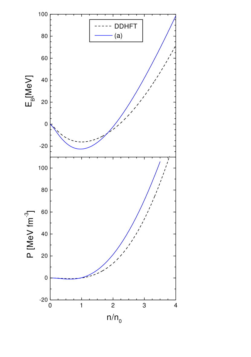
Figure 1: The binding energy (top) and pressure (bottom) for symmetric nuclear matter at zero temperature, evaluated in the MFA using the standard DDHFT treatment and within the approach (a) .

In first place, we have examined the effects of introducing the effective vertices by means of the algebraic Eqs. (19), or by solving a differential equation of the type listed in Eqs. (II)-(II). It must be noted that the first option has the property of reproducing the energy density of the original Dirac-Brueckner calculations, whenever the parameterization of the vertices in terms of only the baryon number density is chosen. Otherwise, it is a definition without any special physical significance. The alternative procedure proposed in AGUIRRE , aims to make a connection between the hadronic vertices and another theoretical framework, by imposing the equality of the nucleon self-energies evaluated in both cases.
For the purpose stated, we have chosen as input the results of TYPEL . In this work, an ansatz for the vertices is proposed that fits several specific Dirac-Brueckner outcomes, but avoiding the unphysical behavior they exhibit in the zero density limit. The ansatze for the couplings $\Gamma_{s}^{TW}$ and $\Gamma_{w}^{TW}$ are rational functions of the relative baryonic density $n_{B}/n_{0}$. The corresponding self-energies are obtained as $\Sigma_{s}^{(in)}=\Gamma_{s}^{TW}\tilde{\sigma}$, $\Sigma_{v}^{(in)}=\Gamma_{w}^{TW}\tilde{\omega}$, with the meson mean field values given by equations similar to those of Eq. (II). For details, see Ref. TYPEL .
In Fig. 1 we show the binding energy and pressure evaluated within the standard DDHFT treatment of TYPEL . Given the functions $\Sigma_{s}^{(in)},\,\Sigma_{v}^{(in)}$ as above, we can also use them to deduce the vertices $\Gamma_{s},\,\Gamma_{w}$ which reproduce these self-energies within the approach (a); i.e. solving Eqs. (II). The corresponding equation of state is shown in the same figure. We have examined densities up to four times $n_{0}$, a range that may be reached inside neutron stars. It can be seen that similar results for the pressure are obtained for densities below $1.25n_{0}$, but the binding energy shows appreciable differences. These results are qualitatively comparable, although for high densities the standard DDHFT treatment gives a softer growth for both $E_{B}$ and $P$. These differences could be significative for those phenomena dominated by the regime of extreme densities, such as the structure of neutron stars.

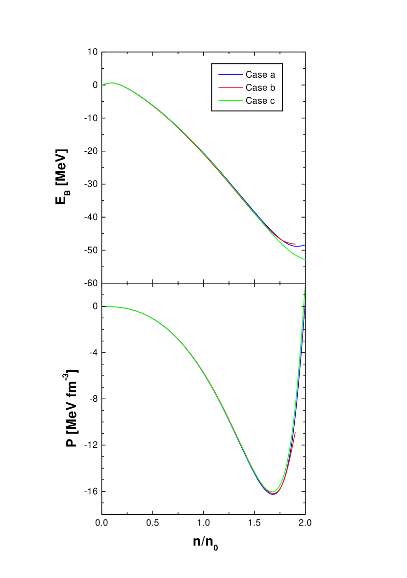
Figure 2: The binding energy (top) and pressure (bottom) obtained by using as input the results of DRUKAREV , within the approaches (a-c).

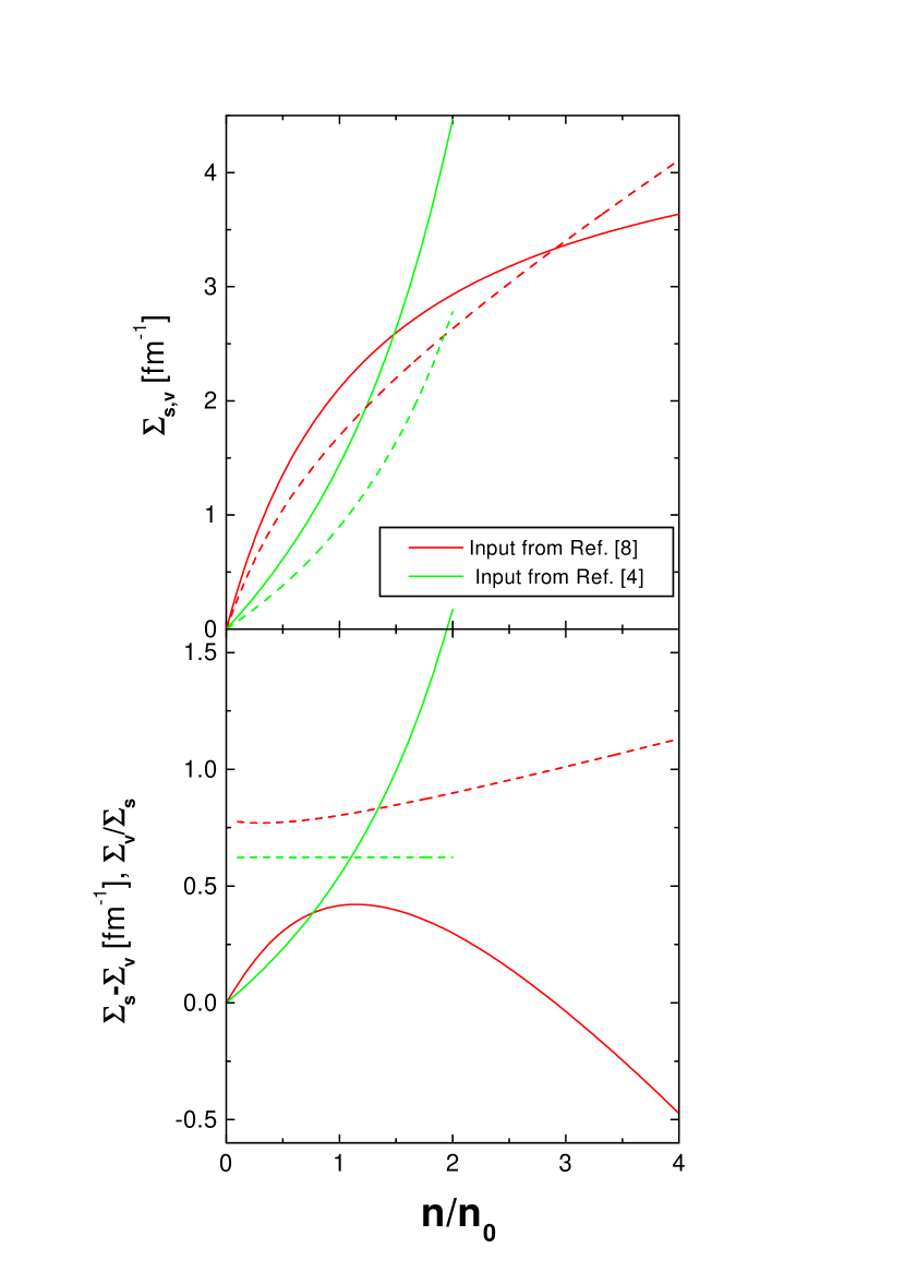
Figure 3: The nucleon self-energies for symmetric nuclear matter, provided by references TYPEL and DRUKAREV . In the upper panel the magnitudes of $\Sigma_{s}^{(in)}$ (solid lines) and $\Sigma_{v}^{(in)}$ (dashed lines), in the lower panel the difference (solid lines) and the quotient (dashed lines) between the scalar and vector components.

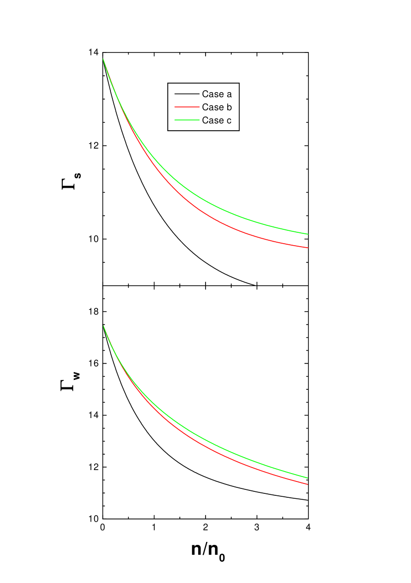
Figure 4: The effective nucleon-meson vertices as functions of the baryonic density, obtained by using the self-energy deduced from TYPEL under the cases (a-c).

As the next subject we have examined the effect of multiple representations. Indeed, given a set of functions $\Sigma_{s},\,\Sigma_{\mu}$ depending on the macroscopic variables of nuclear matter, there exist an indefinite number of models like that of Eq. (II), capable of reproduce them within MFA. Some of these possibilities have been listed as cases (a-c) in the previous section. The formal aspects have been summarized in Eqs. (II)-(II), now we focus on some thermodynamical observables of symmetric nuclear matter.
To avoid biased conclusions we have considered two inputs of diverse source. In addition to the results of TYPEL , based on one-boson exchange potentials, we have included the QCD sum rules calculations of DRUKAREV . We have evaluated the binding energy and the pressure, for each of these inputs under the three assumptions (a-c). We have found that despite the different parameterizations used for a given input, the results are practically undistinguishable in both cases. In Fig. 2 we show this feature for the calculations using the inputs obtained from DRUKAREV , where it can be seen that the three curves are nearly coincident. The range of densities has been restricted to the region of validity of the QCD sum rules computations. The binding energy is monotonically decreasing, it seems to have a minimum near $n\simeq 2\,n_{0}$ where the effective nucleon mass tends to zero. This description does not adjust to the nuclear matter phenomenology, however we keep Ref. DRUKAREV into consideration as it offers a physically meaningful input. It must be noted that the result (c) does not coincide with the preliminary result given in Ref. AGUIRRE , as the $\omega$ meson contribution to the energy was not properly taken into consideration there.
A similar conclusion is obtained by using the self-energies extracted from TYPEL , since the curves corresponding to the instances (b) and (c) (not shown in the figure) follow closely the solid curves of Fig. 1, in the full range $0<n<4\,n_{0}$.
The different behavior between the inputs obtained from DRUKAREV and TYPEL , for the energy per particle, can be justified by examination of Fig. 3. In the upper panel the self-energies as functions of the density, show a monotonous increase in both cases. However the rate of growth of $\Sigma_{s}$ becomes lesser than the corresponding to $\Sigma_{v}$ for densities $n\geq n_{0}$, in the parameterization of TYPEL . The QCD sum rules outputs instead, keeps a faster increase of the scalar as compared to the vector self-energy, over all the domain of densities. This behavior is emphasized in the bottom panel, where the difference $\Sigma_{s}-\Sigma_{v}$ is monotonous increasing in one case, but exhibits a extremum in the other one. Furthermore, a constant quotient $\Sigma_{v}/\Sigma_{s}$ is obtained for the QCD sum rules input, but it increases slowly for the other instance. Anyhow, the rational density dependence of Eq. (18) for the iso-scalar self-energies could be retained in order to simulate the nuclear matter mechanism of saturation, for instance with $\alpha_{s}=-0.278,\,\alpha_{v}=-2.93,$ and $\lambda=0.697$ we have obtained a binding energy of $-14$ MeV at $n\simeq 1.1\,n_{0}$. These values must be contrasted with the parameterization deduced from DRUKAREV , $\alpha_{s}=-2.309,\,\alpha_{v}=-0.66,$ and $\lambda=-0.261$.
The density dependence of the vertices, obtained by using the input of Ref. TYPEL under the three approaches (a-c) is presented in Fig. 4. It must be noted that the expressions for $\Gamma_{s,w}$ become singular at zero density, nevertheless they have finite limits: $\Gamma_{s}^{2}\rightarrow m_{s}^{2}d\Sigma_{s}^{(in)}/dn,\,\Gamma_{w}^{2}\rightarrow m_{w}^{2}d\Sigma_{v}^{(in)}(0)/dn$, for all the cases under consideration.
A common feature of the vertices is a strong decrease up to $n\leq 2\,n_{0}$, which moderates above this value. The cases (b) and (c) yield very similar results for both $\Gamma_{s}$ and $\Gamma_{w}$, differences with the case (a) may lead to qualitatively distinct descriptions for subsequent applications. All these results for the vertices $\Gamma_{k}(z)$ can be summarized by an expression in terms of its natural variable $z$, $\Gamma_{k}=(z+a_{k})/\left(b_{k}+c_{k}(z+a)+d_{k}(z+a)^{2}\right)$, with $k=s,w$ and the numerical coefficients are shown in Table 1.

Case	$a_{s}$	$b_{s}$	$c_{s}$	$d_{s}$	$a_{w}$	$b_{w}$	$c_{w}$	$d_{w}$	$z_{s}$	$z_{w}$
(a)	0.805	-0.170	0.350	-0.082	0.386	-0.032	0.148	-0.024	$s_{1}$	$s_{1}$
(b)	1.264	-0.232	0.294	-0.031	0.413	-0.018	0.096	0.009	$s_{2}$	$s_{1}$
(c)	0.059	0.000	0.066	0.078	1.178	-0.217	0.285	-0.037	$m_{2}$	$m_{1}$

Table 1: Numerical values of the fitting coefficients for the density dependence of the vertices, obtained in the approaches (a-c) using the self-energies deduced from TYPEL .

Another insight into the basic phenomenology of nuclear matter, can be given by the Landau parameters. They can be evaluated as the Legendre projections of the second derivative of $E_{MFA}$ with respect to the baryonic density, for a deduction see MATSUI . These parameters are very useful in regard to collective phenomena of the dense nuclear environment, as for instance, phase transitions, the giant monopolar and quadrupolar modes, or the sound velocity KURASAWA . In order to keep track of the momentum dependence, we assume a non-zero spatial component of the self-energy $\vec{\Sigma}_{v}$, the baryonic current $\vec{j}$ and the omega meson $\vec{\omega}$, taking the zero limit of these quantities at the end of the calculations. So, for example, we write $E_{p}=\sqrt{(\vec{p}-\vec{\Sigma})^{2}+M^{\ast\,2}}$ into the integral of Eq. (20). Denoting by $n_{k}$ the occupation number of nucleon states with a well defined momentum $\vec{p}_{k}$, then we define

$$f_{kl} = \frac{\partial^{2}E_{MFA}}{\partial n_{k}\partial n_{l}}$$

$$= -\frac{M^{\ast}}{E_{i}}\,\frac{\partial\Sigma_{s}}{\partial n_{l}}+\frac{\partial\Sigma_{v}}{\partial n_{l}}-\frac{\vec{p}_{k}}{E_{k}}\cdot\frac{\partial\vec{\Sigma}_{v}}{\partial n_{l}}-\frac{\partial\vec{\Sigma}_{v}}{\partial n_{k}}\cdot\left(\frac{\partial\vec{j}}{\partial n_{l}}-\frac{n_{s}}{M^{\ast}}\frac{\partial\vec{\Sigma}_{v}}{\partial n_{l}}\right)+m_{w}^{2}\frac{\partial\vec{\omega}}{\partial n_{k}}\cdot\frac{\partial\vec{\omega}}{\partial n_{l}},$$

in the second equality, the limit of isotropic nuclear matter has been taken. The derivative of the baryonic current can be evaluated in the MFA

$$\frac{\partial\vec{j}}{\partial n_{i}}=\frac{\vec{p}_{i}}{E_{i}}-H\,\frac{\partial\vec{\Sigma}_{v}}{\partial n_{i}},\;\;\;H=\frac{1}{6\pi^{3}}\int_{0}^{p_{f}}d^{3}p\;\frac{2p^{2}+3M^{\ast\,2}}{(p^{2}+M^{\ast\,2})^{3/2}}.$$

The remaining derivatives are

$$\frac{\partial\vec{\omega}}{\partial n_{i}}=\frac{\tilde{\omega}}{n}\,\frac{\partial\vec{j}}{\partial n_{i}},\;\;\;\frac{\partial\vec{\Sigma}_{v}}{\partial n_{i}}=\frac{\vec{p}_{i}}{E_{i}}\,\frac{\Sigma_{v}}{n+H\,\Sigma_{v}},$$

whose explicit form depends on the approach used (a-c).
The Landau parameters $f_{k}$ are defined by means of the projections

$$f_{m}=\frac{2m+1}{2\pi}\int_{-1}^{1}f_{kl}P_{m}(\nu)d\nu,$$

with $\nu$ the cosine of the angle between $\vec{p}_{k}$ and $\vec{p}_{l}$, and $P_{m}$ the Legendre polynomial of order $m$. At the end of the calculations, the replacement $\mid\vec{p}_{k}\mid,\,\mid\vec{p}_{l}\mid\;\rightarrow p_{F}$ is made. By this procedure, we have obtained the Landau parameters of zero and first orders

$$f_{0} = -\frac{M^{\ast}}{E_{F}}\,\frac{d\Sigma_{s}^{(inp)}}{dn}+\frac{d\Sigma_{v}^{(inp)}}{dn},$$

$$f_{1} = \left(\frac{p_{F}/E_{F}}{n+H\,\Sigma_{v}^{(inp)}}\right)^{2}\left[m_{w}^{2}\tilde{\omega}^{2}-2n\Sigma_{v}^{(inp)}+\left(\frac{n_{s}}{M^{\ast}}-H\right)\Sigma_{v}^{(inp)\,2}\right].$$

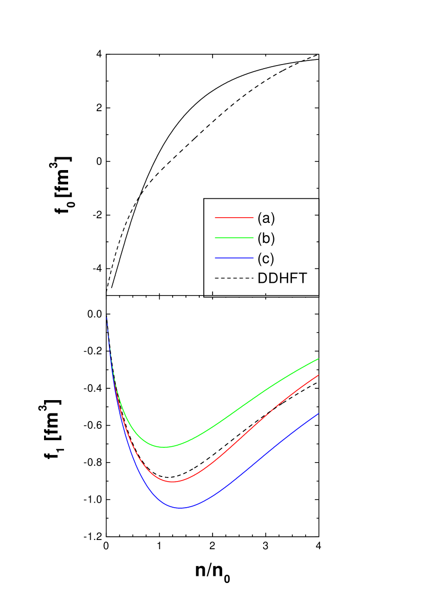
Figure 5: The Landau parameters of zero and first order in terms of the baryonic density, obtained by using the self-energy deduced from TYPEL , and under the cases (a-c) and the standard DDHFT treatment.

It is costumary to normalize the Landau parameters with the density of states at the Fermi surface $\varepsilon_{F}=2p_{F}E_{F}/\pi^{2}$, so that $F_{k}=\varepsilon_{F}f_{k}$.
For a given model of self-energies, the result for $f_{0}$ does not depend on the field parameterization of the vertices. The parameter $f_{1}$ instead, depends on $\tilde{\omega}$ which certainly differs for each of the instances (a-c). In Fig. 5 the density dependence of both Landau parameters is shown, significative departures for $f_{1}$ are found for densities above $0.25n_{0}$.
Consequently all physical magnitudes depending solely on $f_{0}$, such as the nuclear compressibility $K=3p_{F}^{2}(1+F_{0})/E_{F}$, do not distinguish among the field parameterization of the vertices. The same feature is shared by the giant monopole mode energy $E_{M}=\alpha_{0}/A^{1/3}$, with $\alpha_{0}\simeq 1.076\sqrt{K/\mu}$, and the first sound velocity $v_{1}=p_{F}\sqrt{(1+F_{0})/(3\mu E_{F})}$. On the other hand, the excitation energy of the quadrupole state is given by $E_{Q}=\alpha_{2}/A^{1/3}$, with $\alpha_{2}=p_{F}\sqrt{2}/(1.2\mu\sqrt{1+F_{1}/3})$, therefore it is sensitive to the approach used. We have obtained in our calculations $K\simeq 440$ MeV, $\alpha_{0}\simeq 145$ MeV, and $\alpha_{2}\simeq 77$ MeV at the normal density, which must be compared with the empirical values 230 MeV $<K<$ 270 MeV, $\omega_{0}=80$ MeV, and $\omega_{2}=63$ MeV.
Another interesting phenomenological property that can be related to the Landau parameters, are the zero sound modes. These are longitudinal collective modes propagating in nuclear matter at zero temperature, whose dispersion relation can be found as the zeros of the longitudinal dielectric function

$$\varepsilon_{L}=1+\left(F_{0}+\frac{F_{1}\,Q^{2}}{1+F_{1}/3}\right)\Phi(Q)$$

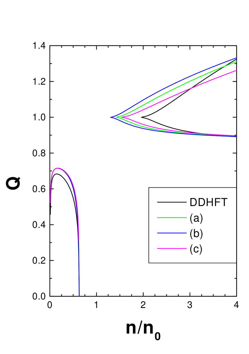
Figure 6: The low lying collective longitudinal modes in terms of the baryonic density, under the cases (a-c) and the standard DDHFT treatment.

with $Q=p_{0}E_{F}/(\mid\vec{p}\mid p_{F})$ and $\Phi$ the Lindhard function. Collective modes have been studied in detail within relativistic field models, see for instance MATSUI ; KURASAWA ; LIM ; CAILLON ; COLLMODES . Low lying collective modes can be classified as instability modes, in the low density regime, and zero sound modes with a characteristic linear dispersion relation $p_{0}\propto\mid\vec{p}\mid$. In Fig. 6, the dispersion relation in terms of the baryonic density is shown for the standard DDHFT treatment and for the approaches (a-c), within the self-energy parametrization of TYPEL . These results are appropriate for the regime $\mid\vec{p}\mid\rightarrow 0$, but keeping the linear dispersion relation. The instability and zero sound modes are clearly distinguishable, as the first one is closely related to the equation of state, all the corresponding curves practically coincide. The zero sound yields very different behaviors, the extremum values for its threshold are obtained within the approaches (b) and the standard DDHFT treatment. We have obtained $n/n_{0}=1.25$ and $2$, respectively. In all the cases we have obtained two-folded zero sound, and taking into account that $\Phi(Q)$ has non zero imaginary part for $Q<1$, only the upper mode is undamped.

IV Conclusions

We have examined in this work, two definitions for the vertices of a hadronic field model in terms of the self-energies provided by another theoretical framework. The first one is the standard DDHFT treatment, which uses Eqs. (19) to define the vertices $\Gamma_{s},\,\Gamma_{w}$ between nucleon and scalar and vector mesons, respectively. There, $\Sigma^{(in)}$ denotes the nucleon self-energies, based on Dirac-Brueckner calculations with one-meson exchange potentials. Although vector and scalar dependencies have been stated LENSKE , most practical applications have used only the first one, similar to our case (a). This particular choice has the property of reproducing the equation of state of the source calculations, but on the contrary the self-energies formally differ from the inputs $\Sigma^{(in)}$. An alternative definition was proposed in AGUIRRE , it consisted in equating both, the input self-energy and that evaluated within the hadronic model with vertices depending on scalar combinations of hadronic fields. This procedure ensures a coherent overlap of the effective hadronic field model and a more fundamental theoretical description, at least in the baryon sector. Three different parametrizations of the vertices, cases (a-c), and two theoretical sources, namely the QCD sum rules of Ref. DRUKAREV and the Dirac-Brueckner parametrization of Ref. TYPEL , have been examined within this scheme.
Thermodynamical aspects of symmetric nuclear matter evaluated in MFA, are undistinguishable for the instances (a-c) within the approach of AGUIRRE , see Eqs.(II-II), but they differ noticeably from the standard DDHFT results. Although the almost perfect coincidence within the (a-c) approaches for the energy and pressure, the vertices obtained present significative deviations in the medium to high densities regime. The results for $\Gamma_{s},\,\Gamma_{w}$ are similar in the (b) and (c) instances, as they use parametrizations in terms of variables strongly related in the MFA. We have given fittings for all the vertices in terms of its corresponding variables.
In reference to the theoretical source for the inputs $\Sigma^{(in)}$, the parameterization given in TYPEL yields observables in agreement with the nuclear matter phenomenology, as expected. The QCD sum rules instead, do not provide an acceptable description, at least in its present status. Taking the nucleon self-energies proposed in DRUKAREV , we have presented formal expresions for the vertices of a hadronic field model for both isoscalar and isovector channels. However, examination of the binding energy obtained for symmetric nuclear matter, show a qualitative mismatching. This assertion is in opposition to the preliminary results of AGUIRRE , where the vector meson contribution to the energy density was not taken into account correctly. However we have shown that the functional dependence of the isoscalar self-energies given in DRUKAREV is not completely reasonless, so as a redefinition of its numerical parameters produce a satisfactory equation of state.
We have also considered in detail the Landau parameters for symmetric nuclear matter, under the four assumptions and the parametrization of TYPEL . The hadronic model yields two non-zero Landau parameters $F_{0}$ and $F_{1}$, the first one has a common behavior while the second one strongly depends on the vertices definition. Therefore, nuclear observables depending on $F_{0}$ only, such as isothermal compressibility, first sound velocity and the giant monopole energy, give almost coincident values. Those quantities depending on $F_{1}$ may discriminate among the different approaches, for instance the zero sound modes exhibit very different threshold densities according to the choice made.
To sum up, we have compared several formal schemes of merging external physical information into hadronic field models. For this purpose we have introduced interaction vertices $\Gamma_{s}$ and $\Gamma_{w}$, which are functionals of the hadronic fields, and we have determined them by else the standard DDHFT procedure or by requiring the reproduction of the self-energies used as input. Either of them, yield comparable results for the binding energy and pressure of symmetric nuclear matter. However, physical quantities can be found able to distinguish among the different approaches.
QCD sum rules calculations for the nucleon self-energy, do not meet the requirements of the procedure, however further refinements could improve its performance.

References

• (1) M.A. Shifman, A.I. Vainshtein, and V.I. Zakharov, Nucl. Phys. B147, 385 (1979).
• (2) B.L. Ioffe, Nucl. Phys. B188, 317 (1981).
• (3) E.G. Drukarev and E.M. Levin, Nucl. Phys. A511, 679 (1990); A532, 695 (1991); Prog. Part. Nucl. Phys. 27, 77 (1991); E. G. Drukarev, M.G. Ryskin, V.A. Sadovnikova, Th. Gutsche, and A. Faessler, Phys. Rev. C 69, 065210 (2004).
• (4) E. G. Drukarev, M.G. Ryskin, and V.A. Sadovnikova, Phys. Rev C 70, 065206 (2004).
• (5) R. Brockmann and H. Toki, Phys. Rev. Lett. 68, 3408 (1992).
• (6) S. Haddad and M. Weigel, Phys. Rev. C 48, 2740 (1993).
• (7) H. Lenske and C. Fuchs, Phys. Lett. B345, 355 (1995).
• (8) S. Typel and H.H. Wolter, Nucl. Phys. A656, 331 (1999).
• (9) B.D. Serot and J.D. Walecka, Adv. Nucl. Phys. 16, 1 (1986); B.D. Serot, Rep. Prog. Phys. 55, 1855 (1982).
• (10) S. Typel, Phys. Rev. C 71, 064301 (2005).
• (11) R. Aguirre, Phys. Lett. B611, 248 (2005).
• (12) G.E. Brown and M. Rho, Phys. Rev. Lett. 66, 2720 (1991).
• (13) G.Q. Li, C.M. Ko, and G.E. Brown, Phys. Rev. Lett. 75, 4007 (1995); Nucl. Phys. A606, 565 (1996); G.Q. Li, C.M. Ko, G.E. Brown, and H. Sorge, Nucl. Phys. A611, 539 (1996).
• (14) T. Matsui, Nucl. Phys. A 370, 365 (1981).
• (15) S. Nishizaki, H. Kurasawa, and T. Suzuki, Nucl. Phys. A462, 687 (1987).
• (16) K. Lim, and C.J. Horowitz, Nucl. Phys. A501, 729 (1989).
• (17) J.C. Caillon, P. Gabinski, and J. Labarsouque, Nucl. Phys. A696, 623(2001); J. Phys. G 29, 2291 (2003).
• (18) V. Greco, M. Colonna, M. Di Toro, and F. Matera, Phys. Rev. C 67, 015203 (2003).
Refer to caption