The ⁴He$(e,e^{\prime}p)^{3}$H Reaction with Full Final–State Interaction

Abstract

An ab initio calculation of the ⁴He$(e,e^{\prime}p)^{3}$H longitudinal response is presented. The use of the integral transform method with a Lorentz kernel has allowed to take into account the full four–body final state interaction (FSI). The semirealistic nucleon-nucleon potential MTI–III and the Coulomb force are the only ingredients of the calculation. The reliability of the direct knock–out hypothesis is discussed both in parallel and in non parallel kinematics. In the former case it is found that lower missing momenta and higher momentum transfers are preferable to minimize effects beyond the plane wave impulse approximation (PWIA). Also for non parallel kinematics the role of antisymmetrization and final state interaction become very important with increasing missing momentum, raising doubts about the possibility of extracting momentum distributions and spectroscopic factors. The comparison with experimental results in parallel kinematics, where the Rosenbluth separation has been possible, is discussed.

I Introduction

Numerous experimental as well as theoretical investigations of $(e,e^{\prime}p)$ exclusive reactions, in both light and heavy nuclei, have been performed extensively in the past, with the aim to extract information about the structure of these systems Frullani and Mougey (1984); Lourie et al. (1986); van der Steenhoven et al. (1986, 1987); Ulmer et al. (1987); Jans et al. (1987); Reffay-Pikeroen et al. (1988); Marchand et al. (1988); van den Brand et al. (1988); van der Steenhoven et al. (1988); Steenhoven et al. (1988); den Herder et al. (1988); Lanen et al. (1989); Magnon et al. (1989); Lanen et al. (1990); van den Brand et al. (1991); Ducret et al. (1993); Leuschner et al. (1994); Le Goff et al. (1994); van Leeuwe et al. (1998) . In particular one has tried to access ground state properties of the target nucleus like spectroscopic factors, shell momentum distributions etc. However, it is well known that such quantities can only be obtained under the hypothesis that the reaction mechanism is dominated by a direct knock–out of the proton and neglecting the interaction in the final state. Such assumptions are usually considered more and more plausible as the momentum transferred by the electron to the system increases and allows to probe “single nucleon” physics. In many nuclei the experimental one–body knock–out spectra indeed show very nicely pronounced peaks, hinting to an independent motion of the nucleons in such systems. In these cases shell momentum distributions and spectroscopic factors have been extracted trying to estimate FSI effects in various ways. Spectroscopic factors which are found smaller than 1 (and they are often found considerably far from 1) are interpreted as due to large “correlation effects” induced by the residual interaction in the ground state of the system.

Unfortunately up to recently the two fundamental assumptions mentioned above could not be checked, because of the impossibility to solve the man–body problem in a quantum mechanical consistent way both for ground and continuum states. The recent progress made in few–body physics allows us to start investigating these assumptions. For $A=2$ and 3 the calculations are fully under control  Arenhövel et al. (2005); Golak et al. both for ground and continuum states, and the problem has been investigated. However, the features of such systems are often considered too different from those of a typical “many–body” nucleus, to be taken as testing grounds for validating assumptions on heavier systems.

In the last decade it has been demonstrated that the procedure to calculate reactions with the help of integral transforms originally proposed in 1985 Efros (1985) can be successfully applied in order to overcome the longstanding stumbling block which prevented ab initio calculations of high energy reactions involving four nucleons and more Efros et al. (1997a, b); Barnea et al. (2001); Bacca et al. (2002, 2004). This has been possible thanks to the integral transform with the Lorentz kernel (we will denote it by LIT) proposed in Ref. Efros et al. (1994) and recently applied also to the two–body break–up of the four–body system in Ref. Quaglioni et al. (2004). Thus it is possible now to treat the full dynamics of a reaction to continuum in a nucleus whose features (binding energy and density) are certainly much closer to those of heavier systems than deuteron and triton or ³He.

It is the purpose of this work to perform a model study of the role of the full treatment of the interaction in the four–body dynamics in the ⁴He$(e,e^{\prime}p)^{3}$H reaction and to discuss the plausibility of the direct knock–out and plane wave assumptions. To this aim we use the semirealistic potential MTI–III Malfliet and Tjon (1969) and concentrate on the longitudinal response function, where meson exchange currents effects are negligible. This response is accessible experimentally if one performs a Rosenbluth separation in parallel kinematics, and has been measured in a number of experiments  Ducret et al. (1993); Magnon et al. (1989). Though the use of a semirealistic potential does not allow to draw precise conclusions we believe that a comparison with data may be instructive and we will also comment on that.

In Sec. II the expression for the $(e,e^{\prime}p)$ cross section is recalled and the formalism describing the integral transform approach with a Lorentz kernel to exclusive reactions is reviewed. Results are given in Sec. III while conclusions are summarized in Sec. IV.

II general formalism

II.1 Cross Section

The sixfold electrodisintegration cross section of ⁴He into the two fragments $p$ and ³H is given by Donnelly (1985); Boffi et al. (1993)

$$\frac{d^{6}\sigma_{p,t}}{dE^{\prime}d\Omega_{e^{\prime}}d{\bf p}_{p}} = \sigma_{M}\left[V_{L}S_{L}(\omega,q,p_{p},\theta_{p})+V_{T}S_{T}(\omega,q,p_{p},\theta_{p})+V_{LT}S_{LT}(\omega,q,p_{p},\theta_{p})\cos\phi\right.$$ (1)

$$\left.+V_{TT}S_{TT}(\omega,q,p_{p},\theta_{p})\cos 2\phi\right]\,.$$

Here $E^{\prime}$ and $\Omega_{e^{\prime}}$ denote energy and solid angle of the electron after the reaction, $\sigma_{M}$ is the Mott cross section and $\phi$ denotes the angle between the electron and ejectile planes. Energy and momentum transferred from the electron to the nuclear system are denoted as $\omega$ and ${\bf q}=q\hat{\bf q}$. The quantity ${\bf p}_{p}=(p_{p},\Omega_{p})$ denotes the momentum of the proton detected in coincidence with the electron, and $\theta_{p}$ is the angle between the outgoing proton and $\hat{\bf q}$. The $V_{\beta}$ are kinematical coefficients and the nuclear dynamics is contained by the structure functions $S_{\beta}$.

Integration over $p_{p}$ leads to the fivefold cross section

$$\frac{d^{5}\sigma_{p,t}}{dE^{\prime}d\Omega_{e^{\prime}}d\Omega_{p}} = \int{\frac{d^{6}\sigma_{p,t}}{dE^{\prime}d\Omega_{e^{\prime}}d{\bf p}_{p}}\frac{p_{p}^{2}}{\left|\frac{\partial E_{m}}{\partial p_{p}}\right|}dE_{m}}$$ (2)

$$= \sigma_{M}\frac{p_{p}^{2}}{\left|\frac{\partial E_{m}}{\partial p_{p}}\right|}\left[V_{L}F_{L}(\omega,q,\theta_{p})+V_{T}F_{T}(\omega,q,\theta_{p})\right.$$

$$\left.+V_{LT}F_{LT}(\omega,q,\theta_{p})\cos\phi+V_{TT}F_{TT}(\omega,q,\theta_{p})\cos 2\phi)\right]\,,$$

where $E_{m}=\omega-T_{p}-T_{t}$ represents the missing energy ($T_{p}$ and $T_{t}$ being the proton and triton kinetic energies). The new structure functions $F_{\beta}$ are simply given by

$$F_{\beta}(\omega,q,\theta_{p})=\int{S_{\beta}(\omega,q,p_{p},\theta_{p})dE_{m}}\,.$$ (3)

Notice that, since $S_{\beta}(\omega,q,p_{p},\theta_{p})$ include the energy conserving $\delta$–function, the integration over $E_{m}$ fixes a unique value of $p_{p}$ for each combination of $\omega,q$ and $\theta_{p}$.

The total contribution of the $p,t$ disintegration channel to the inclusive cross section is

$$\frac{d^{3}\sigma_{p,t}}{dE^{\prime}d\Omega_{e^{\prime}}}=\sigma_{M}\left[V_{L}R^{p,t}_{L}(\omega,q)+V_{T}R^{p,t}_{T}(\omega,q)\right]\,,$$ (4)

with

$$R^{p,t}_{\beta}(\omega,q)=\int{\frac{2\pi p_{p}^{2}}{\left|\frac{\partial E_{m}}{\partial p_{p}}\right|}F_{\beta}(\omega,q,\theta_{p})\sin\theta_{p}d\theta_{p}}\,.$$ (5)

In what follows we concentrate on the longitudinal response $F_{L}(q,\omega,\theta_{p})$, representing the response of the system to the electron-nuclear charge interaction. This can be written as

$${F_{L}(q,\omega,\theta_{p})=\sum_{M_{t},M_{p}}\left|\left\langle\Psi_{p,t}^{-}(E_{p,t})\left|\hat{\rho}({\bf q})\right|\Psi_{\alpha}\right\rangle\right|^{2}}\,,$$ (6)

where the four–body ground state is denoted by $\Psi_{\alpha}$, and $\Psi^{-}_{p,t}$ is the continuum final–state of the minus type pertaining to the proton–triton channel Goldberger and Watson (1964) with the relative proton–triton momentum ${\bf k}=k\hat{\bf k}$. The sum goes over the projections $M_{t}$ and $M_{\mathit{p}}$ of the fragment total angular momenta in the final state. The continuum states $\Psi^{-}_{{\mathit{p}},t}$ are normalized to $\delta({\bf k}-{\bf k}^{\prime})\delta_{M_{t}M^{\prime}_{t}}\delta_{M_{p}M^{\prime}_{p}}$. The quantity $E_{p,t}$ is the final state intrinsic energy

$$E_{p,t}=\frac{k^{2}}{2\mu}+E_{t}\,,$$ (7)

where $\mu$ is the reduced mass of the proton-triton system and $E_{t}$ denotes the ³H ground state energy.

The initial and final states are connected by the nuclear charge operator $\hat{\rho}$ which we take in its non relativistic form

$$\hat{\rho}({\bf q})=\sum_{j=1}^{4}{G_{E}^{p}\,\frac{1+\tau_{j}^{3}}{2}}\exp{(i{\bf q}\cdot{\bf r}_{j}})\,.$$ (8)

Here $\tau^{3}_{j}$ denotes the third component of the $j$-th nucleon isospin, ${\bf r}_{j}$ represents the position of the $j$-th nucleon with respect to the center of mass of the four–body system and $G_{E}^{p}$ is the proton electric form factor. In comparing our results with experimental data we will use the proton form factor $\tilde{G}_{E}^{p}=G_{E}^{p}/(1+(q^{2}-\omega^{2})/4m_{p}^{2})^{1/2}$ (containing first order relativistic correction) with $G_{E}^{p}$ in the usual dipole parametrization.

The main difficulty in the calculation of $F_{L}$ is represented by the continuum wave function $\Psi^{-}_{p,t}(E_{p,t})$ in the transition matrix element

$$T_{p,t}(E_{p,t})=\left\langle\Psi_{p,t}^{-}(E_{p,t})\left|\hat{\rho}\right|\Psi_{\alpha}\right\rangle~{}.$$ (9)

With the integral transform method Efros (1985) with the Lorentz kernel Efros et al. (1994); Piana and Leidemann (2000) one is able to perform an ab initio calculation of this transition matrix element in a large energy range without dealing with the continuum solutions of the four–body Schrödinger equation. How this is possible has been described in Ref. Efros (1985) and will be briefly summarized in the next subsection. Further details can be found in Efros (1993, 1999); Piana and Leidemann (2000); Quaglioni et al. (2004).

II.2 The LIT Method for Exclusive Reactions

The LIT approach to exclusive reactions consists in calculating transition matrix element of the perturbation $\widehat{O}$ between the initial ($\Psi_{0}$) and final ($\Psi^{-}_{f}$) states

$$T_{f}(E_{f})=\left\langle\Psi^{-}_{f}(E_{f})\left|{\widehat{O}}\right|\Psi_{0}\right\rangle~{},$$ (10)

without calculating $\Psi^{-}_{f}(E_{f})$.

In general denoting with $a$ and $b$ the two fragments containing $n_{a}$ and $n_{b}=A-n_{a}$ nucleons, respectively and with $H$ the full nuclear Hamiltonian, we have the following formal expression for $\Psi^{-}_{f=a,b}(E_{f=a,b})$ in terms of the “channel state” $\phi_{f=a,b}^{-}(E_{f=a,b})$ Goldberger and Watson (1964)

$$\left|\Psi^{-}_{a,b}(E_{a,b})\right\rangle={\widehat{\mathcal{A}}}\left|\phi_{a,b}^{-}(E_{a,b})\right\rangle+\frac{1}{E_{a,b}-i\varepsilon-H}\widehat{\mathcal{A}}{\mathcal{V}}\left|\phi_{a,b}^{-}(E_{a,b})\right\rangle\,,$$ (11)

where $\widehat{\mathcal{A}}$ is an antisymmetrization operator. In case that at least one of the fragments is chargeless the channel wave function $\phi_{a,b}^{-}(E_{a,b})$ is the product of the internal wave functions of the fragments and of their relative free motion. Correspondingly, ${\mathcal{V}}$ in Eq. (11) is the sum of all interactions between particles belonging to different fragments. If both fragments are charged, like in our case, $\phi_{a,b}^{-}(E_{a,b})$ is chosen to account for the average Coulomb interaction between them, and the plane wave describing their relative motion is replaced by the Coulomb function of the minus type. Correspondingly, ${\mathcal{V}}$ in Eq. (11) is the sum of all interactions between particles belonging to different fragments after subtraction of the average Coulomb interaction, already considered via the Coulomb function. We write $\phi_{a,b}^{-}(E_{a,b})$ in the partial wave expansion form

$$\phi^{-}_{a,b}(E_{a,b})=\frac{\Phi_{a}(1,...,n_{a})\Phi_{b}(n_{a}+1,...,A)}{(2\pi)^{3/2}}~{}4\pi\sum_{\ell=0}^{\infty}\sum_{m=-\ell}^{\ell}{i^{\ell}e^{-i\delta_{\ell}(k)}\frac{w_{\ell}(k;r)}{kr}Y_{\ell m}(\Omega_{r})Y^{*}_{\ell m}(\Omega_{k})\,.}$$ (12)

Here $\Phi_{a}(1,...,n_{a})$ and $\Phi_{b}(n_{a}+1,...,A)$ are the internal wave functions of the fragments, ${\mathbf{r}}=(r,\Omega_{r})={\mathbf{R}}^{a}_{cm}-{\mathbf{R}}^{b}_{cm}$ represents the distance between them, and the energy of the relative motion is $k^{2}/2\mu=E_{a,b}-E_{a}-E_{b}$, where $E_{a}$ and $E_{b}$ are the fragment ground state energies. The functions $w_{\ell}(k;r)$ are the regular Coulomb wave functions of order $\ell$, and $\delta_{\ell}(k)$ are the Coulomb phase shifts Goldberger and Watson (1964). The internal wave functions of the fragments are assumed to be antisymmetrized and normalized to unity, so that the properly normalized continuum wave function in Eq. (11) is obtained via application of the antisymmetrization operator. For $n_{a}=1$ this has the form

$${\widehat{\mathcal{A}}}=\frac{1}{\sqrt{A}}\left[1-\sum_{j=2}^{A}{\mathcal{P}}_{1j}\right]~{},$$ (13)

where ${\mathcal{P}}_{ij}$ are particle permutation operators Goldberger and Watson (1964).

When one inserts Eq. (11) into Eq. (10) the transition matrix element becomes the sum of two pieces, a Born term,

$$T_{a,b}^{Born}(E_{a,b})=\left\langle\phi_{a,b}^{-}(E_{a,b})\left|{\widehat{\mathcal{A}}}~{}{\widehat{O}}\right|\Psi_{0}\right\rangle~{},$$ (14)

and a FSI dependent term,

$$T_{a,b}^{FSI}(E_{a,b})=\left\langle\phi_{a,b}^{-}(E_{a,b})\left|{\mathcal{V}}{\widehat{\mathcal{A}}}\frac{1}{E_{a,b}+i\varepsilon-H}{\widehat{O}}\right|\Psi_{0}\right\rangle~{}.$$ (15)

While the Born term is rather simple to deal with, the determination of the FSI dependent matrix element is rather complicated. Within the LIT approach this term is treated as outlined in the following.

In Eq. (15) one inserts the completeness relation of the Hamiltonian eigenstates $\Psi_{\nu}(E_{\nu})$ (labelled by channel quantum numbers $\nu$ and normalized as $\langle\Psi_{\nu}|\Psi_{\nu^{\,\prime}}\rangle=\delta(\nu-\nu^{\,\prime})$)

$$T_{a,b}^{FSI}(E_{a,b})=\sum\!\!\!\!~{}\!\!\!\!\!\!\int d\nu\,\langle\phi_{a,b}^{-}(E_{a,b})|{\mathcal{V}}{\widehat{\mathcal{A}}}|\Psi_{\nu}(E_{\nu})\rangle\frac{1}{E_{a,b}+i\varepsilon-E_{\nu}}\langle\Psi_{\nu}(E_{\nu})|{\widehat{O}}|\Psi_{0}\rangle\,.\\$$ (16)

Defining $F_{a,b}(E)$ as

$$F_{a,b}(E)=\sum\!\!\!\!~{}\!\!\!\!\!\!\int d\nu\left\langle\phi_{a,b}^{-}(E_{a,b})\left|{\mathcal{V}}{\widehat{\mathcal{A}}}\right|\Psi_{\nu}(E_{\nu})\right\rangle\left\langle\Psi_{\nu}(E_{\nu})\left|{\widehat{O}}\right|\Psi_{0}\right\rangle\delta(E-E_{\nu})~{},$$ (17)

one has

$$T_{a,b}^{FSI}(E_{a,b}) = \int_{E_{th}^{-}}^{\infty}{\frac{F_{a,b}(E)}{E_{a,b}+i\varepsilon-E}dE}~{}=~{}-i\pi F_{a,b}(E_{a,b})+{\mathcal{P}}\int_{E_{th}^{-}}^{\infty}{\frac{F_{a,b}(E)}{E_{a,b}-E}dE}~{},$$ (18)

where $E_{th}$ is the lowest excitation energy in the system i.e. the break–up threshold energy.

The function $F_{a,b}$ contains information on all the eigenstates $\Psi_{\nu}$ for the whole eigenvalue spectrum of $H$. It is obtained by its Lorentz integral transform

$$L\left[F_{a,b}\right](\sigma)=\int_{E_{th}^{-}}^{\infty}{\frac{F_{a,b}(E)}{(E-\sigma_{R})^{2}+\sigma_{I}^{2}}~{}dE}~{}=~{}\left\langle{\widetilde{\Psi}}_{2}(\sigma)\left|\right.{\widetilde{\Psi}}_{1}(\sigma)\right\rangle~{},$$ (19)

where

$${\widetilde{\Psi}}_{1}(\sigma)=(H-\sigma)^{-1}{\widehat{O}}\left|\Psi_{0}\right\rangle,\qquad{\widetilde{\Psi}}_{2}(\sigma)=(H-\sigma)^{-1}{\widehat{\mathcal{A}}}{\mathcal{V}}|\phi_{a,b}^{-}(E_{a,b})\rangle$$ (20)

and $\sigma=\sigma_{R}+i\sigma_{I}$. Equation (19) shows that $L\left[F_{a,b}\right](\sigma)$ can be calculated without explicit knowledge of $F_{a,b}$, provided that one solves the two equations

$$(H-\sigma)\left|{\widetilde{\Psi}}_{1}\right\rangle = {\widehat{O}}\left|\Psi_{0}\right\rangle~{},$$ (21)

$$(H-\sigma)\left|{\widetilde{\Psi}}_{2}\right\rangle = {\widehat{\mathcal{A}}}{\mathcal{V}}|\phi_{a,b}^{-}(E_{a,b})\rangle\,,$$ (22)

which differ in the source terms only. It is easy to show that ${\widetilde{\Psi}}_{1}$ and ${\widetilde{\Psi}}_{2}$ have finite norms. When solving Eqs. (21) and (22) it is sufficient to require that the solutions are localized, and no other boundary conditions are to be imposed. Therefore “bound state” techniques can be applied.

We use an expansion over a basis set of localized functions consisting of correlated hyperspherical harmonics (CHH) multiplied by hyperradial functions. As discussed in Barnea et al. (2001) for the case of the total ⁴He photoabsorption cross section, special attention has to be paid to the convergence of such expansions. A rather large number of basis states is necessary in order to reach convergence, thus leading to large Hamiltonian matrices. Instead of using a time consuming inversion method we directly evaluate the scalar products in (19) with the Lanczos technique as explained in Ref. Marchisio et al. (2003).

After having calculated $L[F_{a,b}](\sigma)$ one obtains the function $F_{a,b}(E)$, and thus $T_{a,b}(E_{a,b})$, via the inversion of the LIT, as described in Efros et al. (1999).

In the next section results obtained by means of Eq. (14) will be labelled by PWIAS. The label PWIA will indicate that in Eq. (14) the antisymmetrization operator ${\mathcal{A}}$ has been neglected. We remind the reader that in this case the structure function $F_{L}^{p,t}$ turns out to be factorized in terms of the proton form factor and a function $n(|{\bf q}-{\bf p_{p}}|)$, which is the Fourier transform of the overlap between the ⁴He and ³H ground state wave functions.

III results

As already mentioned, the ground states of ⁴He and ³He as well as the $\tilde{\Psi}$ in Eqs. (21) and (22) are calculated using the CHH expansion method. In order to speed up the convergence, state independent correlations are introduced as in Efros et al. (1997a). We use the MTI–III Malfliet and Tjon (1969) potential and identical CHH expansions for the ground state wave functions of ⁴He and of the three–nucleon systems as in Barnea et al. (2001) and Efros et al. (1997c), respectively.

We calculate the transition matrix elements (14) and (15) in the form of partial wave expansions. When one substitutes the expansion (12) and the expansion

$${\hat{\rho}}({\bf q})=\sum_{LM}Y_{LM}^{*}(\Omega_{q}){\hat{\rho}}_{LM}(q)$$ (23)

of the charge operator (8) into the Born amplitude (14) and into the right–hand sides of Eqs. (21) and (22) one finds that in our case of central NN forces the transition matrix element (9) turns into a sum over over $L$ ($L$ is equal to the $l$ in (12)) of partial transition matrix elements multiplied by the factors

$$\sum_{M=-L}^{L}Y_{LM}(\Omega_{k})Y_{LM}^{*}(\Omega_{q})=(4\pi)^{-1}(2L+1)P_{L}({\hat{\bf k}}\cdot{\hat{\bf q}}).$$ (24)

These factors determine the dependence of the cross section on $\theta_{p}$. The dynamic equations are split with respect to orbital momentum $L$ and they are $M$–independent. The multipole transitions of the charge operator in Eq. (8) are taken into account up to a maximal value of $L_{Born}=20$ and $L_{FSI}=6$ for the Born and FSI terms, respectively. (The relatively low value of $L_{FSI}$ is due to the fact that FSI does not affect the final state higher partial waves significantly.) Correspondingly Eqs. (21) and (22) are solved for the different values of $L$, running from $0$ to $L_{FSI}$. Since the excitation operator induces both isoscalar and isovector transitions, the hyperspherical harmonics (HH) entering the calculation are characterized by the quantum numbers $L=0$, $S=0$ and $T=0,1$. In the calculation involving $L$ up to $4$ the maximal value of the grand-angular quantum number $K_{max}$ is taken $7$ (odd multipoles) or $8$ (even multipoles), the only exception being the $L=1$ multipole in the $T=0$ channel, for which $K_{max}=9$ has been used. For $L=5$ and $L=6$ $K_{max}$ is taken equal to $9$ and $10$, respectively. These values of the grand-angular quantum number provide the convergence of the various LIT’s of Eq. (19) with an uncertainty in the response function (6) of less than $1\%$. In addition for $K_{max}=9$ and $10$ a selection of states has been performed with respect to the permutational symmetry types of the HH. Among the HH entering the expansion, those belonging to the irreducible representations [f]=[2] and [f]=[-] Efros et al. (1997a); Fomin and Efros (1981) of the four-particle permutation group S₄ can be neglected in the calculation of the LIT for $K$ values higher than $7$ (odd multipoles) and $8$ (even multipoles).

We start illustrating the contributions of the proton–triton channel and of the mirror channel due to the neutron–³He break–up to the total inclusive response function. This comparison serves as a test of the correctness of the results. In fact below the threshold for the disintegration of ⁴He into proton, neutron and deuteron for the isovector case and into two deuterons for the isocalar case, the two results should coincide. The neutron–³He response $R_{L}^{n,h}(\omega,q)$ has been calculated along the same lines described above, except that in the ”channel state” $\phi_{f=a,b}^{-}(E_{f=a,b})$ of Eq. (11) the relative motion is given by a plane wave. We choose to compare the sum of $R_{L}^{p,t}(\omega,q)$ and $R_{L}^{n,h}(\omega,q)$ for the multipoles L=0, T=1 and L=2, T=0 (two of the multipoles which contribute most) with the total inclusive response calculated for the same multipoles. In Fig. 1 this comparison is shown. Considering that the calculation of the total longitudinal response proceeds in a very different way, i.e. only by inversion of the norm of $\tilde{\Psi}_{1}$ Efros et al. (1997a), this comparison confirms the correctness of the calculation. Besides the degree of accuracy of the results one notices that for these multipoles the proton–triton and neutron–³He channels dominate much beyond those thresholds.

III.1 Parallel kinematics

Our study of $F_{L}(\omega,q,\theta_{p})$ focuses first on the parallel kinematics of Ref. Ducret et al. (1993) where a Rosenbluth separation has been performed. In the columns 2-4 of Table 1 we list the values of $q,\omega$ and modulus of missing momentum ${\bf p}_{m}={\bf q}-{\bf p}_{p}$ of the kinematics we have chosen to analyze (labelled by Kin. N. in column 1). The values of the experimental energies and momentum transfers are illustrated in Fig. 2 as points in the $q-\omega$ plane and labelled with the corresponding numbers. In the same figure their positions with respect to the ridge $\omega=q^{2}/(2m_{p})$ are shown ($m_{p}$ is the proton mass). The value of the final state intrinsic energy $E_{p,t}$, which is the input of the calculation, has been obtained by calculating first the relative momentum ${\bf k}$ from the relation

$${\bf k}=\mu\left(\frac{{\bf p}_{p}}{m_{p}}-\frac{({\bf q}-{\bf p}_{p})}{m_{t}}\right)$$ (25)

and then using Eq. (7).

In column 5 of Table 1 the PWIA results are listed. In this approximation and in an independent particle model of ⁴He the PWIA result represents the probability that the proton in the S-shell of ⁴He has momentum $p_{m}$. Therefore one has constant values for Kin. N. 1-3 and 4-8. The integral over all values of ${\bf p}_{m}$ gives the “spectroscopic factor” for that shell, which for this potential turns out to be 0.88 Efros et al. (1998) (this value can be compared with 0.84 obtained using a realistic potential like AV18 and Urbana IX Schiavilla et al. (1986); Wiringa (1991); Arriaga et al. (1995)).

In Table 1 the effects of antisymmetrization and of FSI are also shown as percentages of the PWIA values (the results denoted as FULL include both effects). In general one notices small effects of antisymmetrization for almost all cases as one would expect for kinematics with $p_{m}$ much smaller than $q$. Nevertheless for the kinematics at lower energies these effects can increase up to about 10%. The role of FSI is much more important, especially at low $q$. One notices that i) for the kinematics close to the $\omega=q^{2}/(2m_{p})$ ridge FSI effects decrease for increasing $q$; ii) Kin. N. 4 and 9, which are more distant from the ridge $\omega=q^{2}/(2m_{p})$, present a rather high contribution of FSI; iii) at higher momenta and in the lower energy side of the ridge FSI enhances the PWIA results. This effect goes in the opposite direction compared to previous estimates based either on optical potentials and orthogonalization procedure Schiavilla (1990), or on diagrammatic expansions Laget (1989).

The observation iii) is consistent with previous ab initio calculations of the inclusive longitudinal response function in ²H  Arenhövel et al. (2005), ³He  Golak et al. (2005)) and ⁴He Efros et al. (1997a). In the latter case one finds that the longitudinal responses at constant $q$ values, calculated with and without FSI, cross at an $\omega$ value of approximately $q^{2}/(2m_{p})$. The fact that the crossing happens just along that ridge is probably due to the different effects of the potential in the initial and in the final state with respect to the free one–body knock–out model, as explained in the following. In the one body knock–out model the PWIA peak energy is $\omega_{peak}=q^{2}/(2m_{p})+\Delta$. The positive quantity $\Delta$ is the difference between the binding energies of ⁴He and ³H and can be considered as a ”ground state effect” of the potential. One can argue that the additional effect of the potential in the final state would lead to $\omega_{peak}=q^{2}/(2m_{p})+\Delta-\bar{V}$, where $\bar{V}$ represents the mean interaction energy between the proton and the triton in the final state interaction zone ($\bar{V}$ will be attractive). Therefore the PWIA and FSI curves should intersect at an energy smaller than $q^{2}/(2m_{p})+\Delta$. To a good accuracy this value turns out to be just $q^{2}/(2m_{p})$. Of course such a comparison between inclusive and exclusive results is justified only in case of sufficiently low $p_{m}$ as it is the case for the kinematics listed in Table 1.

Similar PWIAS and FSI effects are also found for Kin. N. 6 and 9 in the two–body break–up results of ³He Golak et al. (1995).

It is a common belief that the kinematical regions at lower energy and higher momentum transfers are the privileged ones to investigate the ground state short range correlation effects. Our results show that if one relies on approximate approaches to estimate the FSI effects one might underestimate considerably the momentum distributions at high $p_{m}$ extracted from experiment in those kinematical regions.

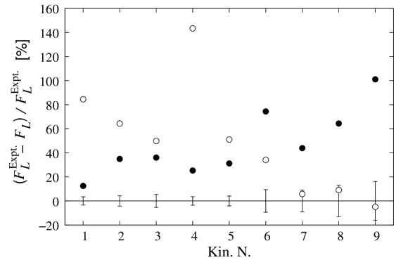
Figure 3: Percentage deviation from the experimental values of Ref. Ducret et al. (1993): PWIA (open circles), FULL results (full circles).

As stated above, the aim of the present work is mainly to study relative effects of antisymmetrization and FSI, which are often treated approximately, via a complete solution of the quantum mechanical few-body problem. We have conducted this study using a semirealistic potential model. Nevertheless it is interesting to compare our results with experiment. This comparison is shown in Table 2. Except for the case at the lowest $\omega$ and $q$ (Kin. N. 1) where there is a good agreement, our results are almost systematically higher than data. The difference ranges from about 30% for the kinematics closer to the quasi elastic ridge to about 70 and even 100% for the other ones. This comparison is better illustrated in Fig. 3. One can see that, while FSI tends to bring theoretical results closer to data for the kinematics at lower momenta (Kin. N. 1-5), it affects in the opposite direction those at higher $q$ (Kin. N. 6-9), with the largest effect for Kin. N. 9 which corresponds to the highest $q$ and $p_{m}$-values. This is a delicate region where cross sections are small and potential dependence and relativistic effects neglected here might play a major role.

III.2 Non parallel kinematics

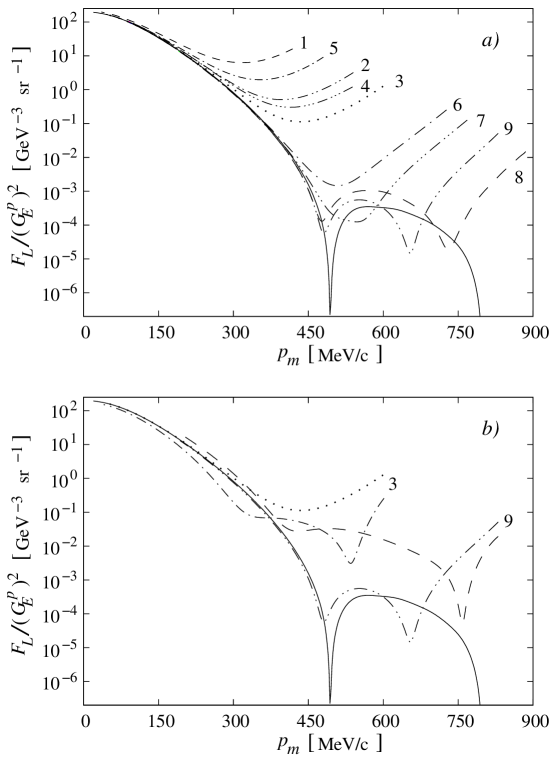
Figure 4: The ⁴He$(e,e^{\prime}p)^{3}$H longitudinal response function of Eq. (6) as function of $p_{m}$: a) PWIAS for the different $(\omega,q)$ values of Table 1 labelled with the corresponding numbers; b) PWIAS (dotted and dot–dot–dashed line) and FULL (dashed and dot–dashed line) results for the $(\omega,q)$ values of Kin. N. 3 and 9 of Table 1. The solid line represents the PWIA.

It is interesting to investigate the above effects also in non parallel kinematics. At fixed energy and momentum transfer one can access different $p_{m}$ varying $\theta_{p}$. Therefore in PWIA the response reflects a proton momentum distribution. In the following we will show how antisymmetrization and FSI can spoil this interpretation. For the $(\omega,q)$ values of Table 1 in Fig. 4 results for non parallel kinematics are shown as functions of $p_{m}$. In the upper panel one can clearly see that the mere antisymmetrization effect does not allow the interpretation of the response in terms of momentum distribution beyond certain values of $p_{m}$, depending on the kinematics. These values are rather small (around 1 fm^-1) for the kinematics at lower momentum transfer and can reach 2 fm^-1 for those at higher $q$. This is of course discouraging for a study of the short range correlations, which contribute mainly to the higher tail of the momentum distribution.

Fig. 4 shows that antisymmetrization effects tend to fill the minimum of the response in PWIA. In order to illustrate the FSI effect, in the lower panel we have chosen Kin. N. 3 with a smaller and Kin. N. 9 with a larger $q$–value. As in parallel kinematics FSI tends to decrease the response in the former case and to enhance it in the latter. It is interesting to see that some minima reappear and some are filled when FSI is included.

For a better understanding of the situation it is instructive to plot the matrix elements calculated from Eqs. (10), (14) and (15). As an example we choose Kin. N. 3. In Fig. 5a our results for $T^{Born}_{p,t}$ are shown for PWIA and PWIAS. Moreover, in order to see the difference between an independent particle model and a correlated one, we also show the corresponding results obtained in an harmonic oscillator (h.o.) model. (The h.o. parameters have been fixed to the radii of ⁴He and ³H). Since the MTI–III potential has a rather strongly repulsive core the comparison exhibits the effect of ground state short range correlations. One readily sees that at low $p_{m}$ the MTI–III potential gives a 15% quenching. The tail region is amplified in the inset. The results of the two models have similar behaviors with increasing $p_{m}$, both in PWIA and PWIAS (see also inset of Fig. 5a). However, while the h.o. PWIA matrix element remains always positive the corresponding one for MTI–III crosses the zero axis, giving origin to the minimum visible in Fig. 4. The minimum is then washed out by the antisymmetrization effect.

In Fig. 5b the additional role of FSI is shown. In this case the total matrix element $T^{Born}_{p,t}+T^{FSI}_{p,t}$ is complex. Real and imaginary parts are shown and compared to the Born result with the MTI–III potential. In the inset the complicate interplay of the different contributions is illustrated. It is evident that FSI leads to a result close to zero for a rather wide $p_{m}$ range, causing appearances and disappearances of minima in the cross section. A more realistic interaction may change the present picture in that kinematical region considerably. Nonetheless this model study points out that it might be difficult to search for ground state correlation effects at high $p_{m}$ values within a PWIA picture.

IV Conclusions

We have presented the results of an ab initio calculation of the ⁴He$(e,e^{\prime}p)^{3}$H longitudinal response obtained by means of the integral transform method with a Lorentz kernel. As NN interaction the MTI-III potential model is used. The aim has been to investigate the limits of the PWIA approximation (factorization in terms of momentum distribution) due to the effects of antisymmentrization and FSI. We have analyzed the situation for the parallel kinematics investigated in the experiments of Ref. Ducret et al. (1993) and for two non parallel kinematics. Our model study has shown that the factorized approach (PWIA) might be a reasonable approximation for small missing momenta (below 0.5 fm^-1) and higher momentum transfers (above 2 fm^-1). Unfortunately the situation for higher missing momenta becomes much more involved. Both antisymmetrization effects and FSI play an important role. In particular for non parallel kinematics their entanglement can give rise to drastic deviations from the PWIA result. Furthermore, one may expect considerable sensitivity to nuclear dynamics here. On the one hand this result can be considered discouraging in relation to the possibility to ”measure” directly short range ground state correlations. On the other hand it is possible that, due to the sensitivity of the response to all effects, those kinematical regions are ideal to study potential model dependence, including perhaps that due to thre–body forces. However, FSI has to be treated in a proper way and realistic interactions have to be used before definite conclusions can be drawn. The integral transform approach with a Lorentz kernel is a promising approach to pursue such studies.

													PWIA
Kin.			$q$		$\omega$			$p_{m}$					$F_{L}/(G_{E}^{\,p})^{2}$										$\Delta_{\rm PWIAS}$							$\Delta_{\rm FULL}$
N.			$({\rm MeV}/c)$		(MeV)			$({\rm MeV}/c)$					$[\left({\rm GeV}/c\right)^{-3}{\rm sr}^{-1}]$										$(\%)$							$(\%)$
$1$			299		57.	78				$+$	30								$185$.	$2$				$+$	$9$.	$3$				$-$	$39$.	$6$
$2$			380		83.	13				$+$	30								$185$.	$2$				$+$	$1$.	$2$				$-$	$20$.	$1$
$3$			421		98.	19				$+$	30								$185$.	$2$				$+$	$0$.	$0$				$-$	$12$.	$8$
$4$			299		98.	70				$-$	90								$100$.	$0$				$+$	$4$.	$5$				$-$	$43$.	$4$
$5$			380		65.	06				$+$	90								$100$.	$0$				$+$	$3$.	$9$				$-$	$16$.	$6$
$6$			544		126.	6				$+$	90								$100$.	$0$				$-$	$1$.	$1$				$+$	$11$.	$4$
$7$			572		137.	82				$+$	90								$100$.	$0$				$-$	$1$.	$9$				$+$	$11$.	$5$
$8$			650		175.	67				$+$	90								$100$.	$0$				$-$	$1$.	$7$				$+$	$10$.	$8$
$9$			680		146.	48				$+$	190								$14$.	$63$				$-$	$4$.	$4$				$+$	$52$.	$1$

Table 1: The ⁴He$(e,e^{\prime}p)^{3}$H longitudinal response function of Eq. (6) in PWIA approximation for the parallel kinematics of Fig. 2. The relative PWIAS and FULL effects, $\Delta_{\rm X}=\left({\rm X}-{\rm PWIA}\right)/{\rm PWIA}$, are also listed.

Kin.					$F_{L}$ $[\left({\rm GeV}/c\right)^{-3}{\rm sr}^{-1}]$
No.					Expt.											FULL
1					59.	0	$\pm$	2.	0	$\pm$	2.	2					66.	4
2					49.	6	$\pm$	2.	1	$\pm$	2.	1					66.	9
3					46.	2	$\pm$	2.	5	$\pm$	2.	2					62.	7
4					27.	8	$\pm$	1.	0	$\pm$	1.	2					34.	9
5					28.	4	$\pm$	1.	2	$\pm$	1.	3					37.	2
6					14.	8	$\pm$	1.	4	$\pm$	1.	2					25.	9
7					16.	0	$\pm$	1.	5	$\pm$	1.	3					23.	0
8					9.	96	$\pm$	1.	29	$\pm$	1.	15					16.	3
9					1.	35	$\pm$	0.	22	$\pm$	0.	22					2.	73

Table 2: The ⁴He$(e,e^{\prime}p)^{3}$H longitudinal response function. Theoretical results (FULL) compared to the experimental values of Ref. Ducret et al. (1993): statistical and systematic uncertainties are indicated ($\pm$stat. $\pm$syst.)

Figure 1: $T=1$, $L=0$ [panel a)] and $T=0$, $L=2$ [panel b)] components of the inclusive response (solid line) compared to those of $R^{p,t}_{L}+R^{n,h}_{L}$ [see Eq. (5)] (dashed line) for $q=300$ MeV/$c$. The arrows indicate the proton-neutron-deuteron (p,n,d,) and deuteron-deuteron (d,d) break–up thresholds.

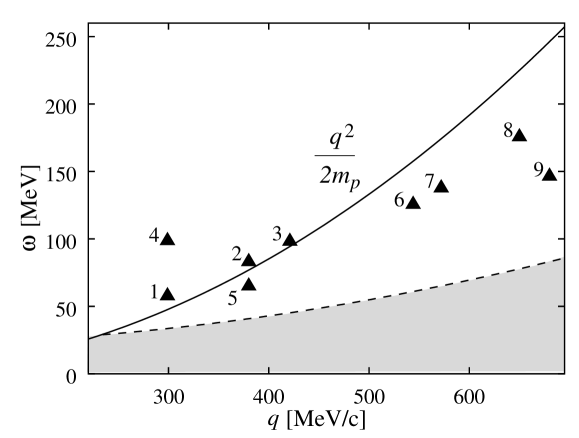
Figure 2: Position of the various kinematics of Table 1 with respect to the $\omega=q^{2}/(2m_{p})$ ridge. The shaded area represents the region below the break–up threshold, where the cross section is zero.

Figure 5: Matrix element $T(E)$ of Eq.(9) in non parallel kinematics, for $q$ and $\omega$ of Kin. N. 3, as function of $p_{m}$. a): h.o. model: PWIA (dashed line), PWIAS (dotted line); MTI–III potential model: PWIA (full line), MTI–III, PWIAS (dot–dashed line). b) MTI–III potential model: real (dashed line) and imaginary (dot-dashed line) parts of the FULL matrix element. PWIA and PWIAS results as in a).

References

- Frullani and Mougey (1984) S. Frullani and J. Mougey, Adv. Nucl. Phys. 14, 1 (1984).
- Lourie et al. (1986) R. W. Lourie, H. Baghaei, W. Bertozzi, K. I. Blomqvist, J. M. Finn, C. E. Hyde-Wright, N. Kalantar-Nayestanaki, J. Nelson, S. Kowalski, C. P. Sargent, et al., Phys. Rev. Lett. 56, 2364 (1986).
- van der Steenhoven et al. (1986) G. van der Steenhoven, H. P. Blok, J. F. J. van den Brand, T. de Forest Jr., J. W. A. den Herder, E. Jans, P. H. M. Keizer, L. Lapikás, P. J. Mulders, E. N. M. Quint, et al., Phys. Rev. Lett. 57, 182 (1986).
- van der Steenhoven et al. (1987) G. van der Steenhoven, A. M. van den Berg, H. P. Blok, S. Boffi, J. F. J. van den Brand, R. Ent, T. de Forest Jr., C. Giusti, J. W. A. den Herder, E. Jans, et al., Phys. Rev. Lett. 58, 1727 (1987).
- Ulmer et al. (1987) P. E. Ulmer, H. Baghaei, W. Bertozzi, K. I. Blomqvist, J. M. Finn, C. E. Hyde-Wright, N. Kalantar-Nayestanaki, S. Kowalski, R. W. Lourie, J. Nelson, et al., Phys. Rev. Lett. 59, 2259 (1987).
- Jans et al. (1987) E. Jans, M. Bernheim, M. K. Brussel, G. P. Capitani, E. D. Sanctis, S. Frullani, F. Garibaldi, J. Morgenstern, J. Mougey, I. Sick, et al., Nucl. Phys. A475, 687 (1987).
- Reffay-Pikeroen et al. (1988) D. Reffay-Pikeroen, M. Bernheim, S. Boffi, G. P. Capitani, E. D. Sanctis, S. Frullani, F. Garibaldi, A. Gérard, C. Giusti, H. Jackson, et al., Phys. Rev. Lett. 60, 776 (1988).
- Marchand et al. (1988) C. Marchand, M. Bernheim, P. C. Gérard, J. M. Laget, A. Magnon, J. Morgenstern, J. Mougey, J. Picard, D. Reffay-Pikeroen, S. Turck-Chieze, et al., Phys. Rev. Lett. 60, 1703 (1988).
- van den Brand et al. (1988) J. F. J. van den Brand, H. P. Blok, R. Ent, E. Jans, G. J. Kramer, J. B. J. M. Lanen, L. Lapikás, E. N. M. Quint, G. van der Steenhoven, and P. K. A. de Witt Huberts, Phys. Rev. Lett. 60, 2006 (1988).
- van der Steenhoven et al. (1988) G. van der Steenhoven, H. P. Blok, E. Jans, M. de Jong, L. Lapikás, E. N. M. Quint, and P. K. A. de Witt Huberts, Nucl. Phys. A480, 547 (1988).
- Steenhoven et al. (1988) G. V. D. Steenhoven, H. P. Blok, E. Jans, L. Lapikás, E. N. M. Quint, and P. K. A. D. W. Huberts, Nucl. Phys. A484, 445 (1988).
- den Herder et al. (1988) J. W. A. den Herder, H. P. Blok, E. Jans, P. H. M. Keizer, L. Lapikás, E. N. M. Quint, G. V. D. Steenhoven, and P. K. A. D. W. Huberts, Nucl. Phys. A490, 507 (1988).
- Lanen et al. (1989) J. B. J. M. Lanen, A. M. van den Berg, H. P. Blok, J. F. J. van den Brand, C. T. Christou, A. G. M. v. H. R. Ent, E. Jans, G. J. Kramer, L. Lapikás, D. R. Lehman, et al., Phys. Rev. Lett. 62, 2925 (1989).
- Magnon et al. (1989) A. Magnon, M. Bernheim, M. K. Brussel, G. P. Capitani, E. D. Sanctis, S. Frullani, F. Garibaldi, A. Gerard, H. E. Jackson, J. M. Le Goff, et al., Phys. Lett. B 222, 352 (1989).
- Lanen et al. (1990) J. B. J. M. Lanen, H. P. Blok, E. Jans, L. Lapikás, G. van der Steenhoven, and P. K. A. de Witt Huberts, Phys. Rev. Lett. 64, 2250 (1990).
- van den Brand et al. (1991) J. F. J. van den Brand, H. P. Blok, H. J. Bulten, R. Ent, E. Jans, G. J. Kramer, J. M. Laget, J. B. J. M. Lanen, L. Lapikás, J. S. Roebers, et al., Phys. Rev. Lett. 66, 409 (1991).
- Ducret et al. (1993) J. E. Ducret, M. Bernheim, M. K. Brussel, G. P. Capitani, J. F. Danel, E. D. Sanctis, S. Frullani, F. Garibaldi, F. Ghio, H. E. Jackson, et al., Nucl. Phys. A556, 373 (1993).
- Leuschner et al. (1994) M. Leuschner, J. R. Calarco, , F. W. Hersman, E. Jans, G. J. Kramer, L. Lapikás, G. van der Steenhoven, P. K. A. de Witt Huberts, H. P. Blok, et al., Phys. Rev. C 49, 955 (1994).
- Le Goff et al. (1994) J. M. Le Goff, M. Bernheim, M. K. Brussel, G. P. Capitani, J. F. Danel, E. D. Sanctis, S. Frullani, F. Garibaldi, A. Gerard, M. Jodice, et al., Phys. Rev. C 50, 2278 (1994).
- van Leeuwe et al. (1998) J. J. van Leeuwe, H. P. Blok, J. F. J. van den Brand, H. J. Bulten, G. E. Dodge, R. Ent, W. H. A. Hesselink, E. Jans, W. J. Kasdorp, J. M. Laget, et al., Phys. Rev. Lett. 80, 2543 (1998).
- Arenhövel et al. (2005) H. Arenhövel, W. Leidemann, and E. L. Tomusiak, Eur. Phys. J. A 23, 147 (2005).
- (22) J. Golak, H. Witala, R. Skibiński, W. Glöckle, A. Nogga, and H. Kamada, eprint nucl-th/0403022.
- Efros (1985) V. D. Efros, Yad. Fiz. 41, 1498 (1985) [Sov. J. Nucl. Phys. 41, 949 (1985)].
- Efros et al. (1997a) V. D. Efros, W. Leidemann, and G. Orlandini, Phys. Rev. Lett. 78, 432 (1997a).
- Efros et al. (1997b) V. D. Efros, W. Leidemann, and G. Orlandini, Phys. Rev. Lett. 78, 4015 (1997b).
- Barnea et al. (2001) N. Barnea, V. D. Efros, W. Leidemann, and G. Orlandini, Phys. Rev. C 63, 057002 (2001).
- Bacca et al. (2002) S. Bacca, M. A. Marchisio, N. Barnea, W. Leidemann, and G. Orlandini, Phys. Rev. Lett. 89, 052502 (2002).
- Bacca et al. (2004) S. Bacca, H. Arenhövel, N. Barnea, W. Leidemann, and G. Orlandini, Phys. Lett. B 603, 159 (2004).
- Efros et al. (1994) V. D. Efros, W. Leidemann, and G. Orlandini, Phys. Lett. B 338, 130 (1994).
- Quaglioni et al. (2004) S. Quaglioni, W. Leidemann, G. Orlandini, N. Barnea, and V. D. Efros, Phys. Rev. C 69, 044002 (2004).
- Malfliet and Tjon (1969) R. A. Malfliet and J. Tjon, Nucl. Phys. A127, 161 (1969).
- Donnelly (1985) T. W. Donnelly, Prog. Part. Nucl. Phys. 13, 183 (1985).
- Boffi et al. (1993) S. Boffi, C. Giusti, and F. D. Pacati, Phys. Rep. 226, 1 (1993).
- Goldberger and Watson (1964) M. L. Goldberger and K. W. Watson, Collision Theory (Wiley, New York, 1964).
- Piana and Leidemann (2000) A. L. Piana and W. Leidemann, Nucl. Phys. A677, 423 (2000).
- Efros (1993) V. D. Efros, Yad. Fiz. 56, N7, 22 (1993) [Phys. At. Nucl. 56, 869 (1993)].
- Efros (1999) V. D. Efros, Yad. Fiz. 62, 1975 (1999) [Phys. At. Nucl. 62, 1833 (1999)].
- Marchisio et al. (2003) M. A. Marchisio, N. Barnea, W. Leidemann, and G. Orlandini, Few-Body Syst. 33, 259 (2003).
- Efros et al. (1999) V. D. Efros, W. Leidemann, and G. Orlandini, Few-Body Syst. 26, 251 (1999).
- Efros et al. (1997c) V. D. Efros, W. Leidemann, and G. Orlandini, Phys. Lett. B 408, 1 (1997c).
- Fomin and Efros (1981) B. A. Fomin and V. D. Efros, Yad. Fiz. 34, 587 (1981) [Sov. J. Nucl. Phys. 34, 327 (1981)].
- Efros et al. (1998) V. D. Efros, W. Leidemann, and G. Orlandini, Phys. Rev. C 58, 582 (1998).
- Schiavilla et al. (1986) R. Schiavilla, V. R. Pandharipande, and R. B. Wiringa, Nucl. Phys. A449, 219 (1986).
- Wiringa (1991) R. B. Wiringa, Phys. Rev. C 43, 1585 (1991).
- Arriaga et al. (1995) A. Arriaga, V. R. Pandharipande, and R. B. Wiringa, Phys. Rev. C 52, 2362 (1995).
- Schiavilla (1990) R. Schiavilla, Phys. Rev. Lett. 65, 835 (1990).
- Laget (1989) J. Laget, Nucl. Phys. A497, 391c (1989).
- Golak et al. (2005) J. Golak, R. Skibinski, H. Witala, W. Glöckle, A. Nogga, and H. Kamada (2005), eprint nucl-th/0505072.
- Golak et al. (1995) J. Golak, H. Kamada, H. Witala, W. Glöckle, and S. Ishikawa, Phys. Rev. C 51, 1638 (1995) and private communication.