Behavior of shell-model configuration moments

Abstract

An important input into reaction theory is the density of states or the level density. Spectral distribution theory (also known as nuclear statistical spectroscopy) characterizes the secular behavior of the density of states through moments of the Hamiltonian. One particular approach is to partition the model space into subspaces and find the moments in those subspaces; a convenient choice of subspaces are spherical shell-model configurations. We revisit these configuration moments and find, for complete $0\hbar\omega$ many-body spaces, the following behaviors: (a) the configuration width is nearly constant for all configurations; (b) the configuration asymmetry or third moment is strongly correlated with the configuration centroid; (c) the configuration fourth moment, or excess is linearly related to the square to the configuration asymmetry. Such universal behavior may allow for more efficient modeling of the density of states in a shell-model framework.

I Introduction and Motivation

An important input into Hauser-Feshbach calculations of statistical capture of neutrons Hauser and Feshbach (1952); T. Rauscher, F.-K. Thielemann and K.-L. Kratz (1997) is the density of nuclear states, or the nuclear level density, as a function of excitation energy. (The phrases “state density” and “level density” are often used informally as synonyms, although they are not: the state density includes $2J+1$ degeneracies, where $J$ is the angular momentum. Because the Hauser-Feshbach formalism uses $J$-dependent transmission coefficients, one ultimately requires the level density as a function of $J$. As will become clear below, we discuss both the total state density as well as $J$-projected level densities.)

The density of states is difficult to obtain both experimentally and theoretically and is perhaps the most uncertain input into Hauser-Feshbach calculations T. Rauscher, F.-K. Thielemann and K.-L. Kratz (1997). Therefore there is significant effort, both experimental and theoretical, going into determining the density of states.

The most common theoretical approaches are built around noninteracting Fermi gases, starting from Bethe’s formulaBethe (1936) using the single-particle density of states. Of course the residual interaction plays a significant role, and single-particle approaches necessarily add corrections to account for the residual interactionGoriely (1996); P. Demetriou and S. Goriely (2001).

An alternative is to start from a fully interacting picture such as the configuration-mixing shell model. Interacting shell-model codes, such as OXBASHB. A. Brown, A. Etchegoyen, and W. D. M. Rae (1984), ANTOINEE. Caurier and F. Nowacki (1999), and REDSTICKOrmand , read in single-particle energies and two-body matrix elements and compute matrix elements of the many-body Hamiltonian in a truncated, albeit very large, many-body basis. All such codes use the Lanczos algorithm to extract the low-lying spectraR.R. Whitehead, A.  Watt, B.J. Cole, and I. Morrison (1977). Obtaining the complete spectrum is unfeasible for large dimension bases, and unnecessary as well: one only needs the smooth, secular behavior of the density of states, not the individual states. Instead, one turns to formulations of the interacting shell model that do not involve diagonalization: auxiliary-field path integrals Ormand (1997); Nakada and Alhassid (1997, 1998), or spectral distribution theory (also known as nuclear statistical spectroscopyJ. B. French and K. F. Ratcliff (1971); S. Ayik and J.N. Ginocchio (1974); K. K. Mon and J. B. French (1975); Wong (1986)).

Nuclear statistical spectroscopy starts from the moments of the Hamiltonian. For example, it is known that, in a finite space, most state densities of many-body systems with a two-body interaction tend toward a Gaussian shape K. K. Mon and J. B. French (1975); Kota (1984) characterized by the first and second moments of the Hamiltonian. In most realistic cases the density has small but non-trivial deviations from a Gaussian, so one requires higher moments. It has long been realized that, rather than computing higher and higher moments of the total Hamiltonian, one could partition the model space into suitable subspaces and compute just a few moments in each subspace. In particular, if one partitions the space based upon spherical shell-model configurations, that is, all states of the form $(0d_{5/2})^{4}(1s_{1/2})^{2}(0d_{3/2})^{2}$, etc., then it is possible to derive expressions for the configuration moments directly in terms of the single-particle energies and two-body matrix elements, without constructing any many-body matrix elements (see, however, our discussion in depth below).

Although such an approach has obvious merit, it is far from trivial. For a realistic application, one must include thousands of configurations. For example, ⁵⁴Fe in a $1s0d$-$1p0f$ space allowing at most two particles to be excited out of the $sd$-shell into the $pf$ consists of 147,060 configurations (which in turn represent $9.5\times 10^{11}$ levels). Furthermore, higher moments take more and more computational effort. The configuration centroids and widths (first and second moments, respectively) take CPU-minutes, while configuration asymmetries (third moments) take CPU-hours or days and configuration 4th moments even longer; in our example of ⁵⁴Fe it takes about 43 minutes on a single 2.4 GHz Pentium to compute all the second moments, but 9 days to compute the third moments.

Therefore one important question is: how many moments must be reliably calculated? A related question is: what is an appropriate model for the secular behavior? Most work has been based on modified Gaussians, in the Gram-Charlier or Edgeware distributions. Kota, Potbhare, and ShenoyV. K. B. Kota, V. Potbhare and P. Shenoy (1986) made a study of model functions and concluded the Cornish-Fisher distribution as the best approximation; they also made a study of the behavior of the configuration moments, and this paper can be considered an further investigation of that early work. ZukerZuker (2001) proposed binomial distributions as a way to naturally include asymmetries. Recently Horoi, Kaiser, and Zelevinsky Horoi et al. (2003) have modeled the level density as a sum of Gaussians, based only upon first and second moments, and ignoring higher moments such as the asymmetry; they argue that the asymmetries tend to cancel.

Given this background, we have investigated in more detail the configuration moments and their distributions. Before sharpening our questions further, we lay out more carefully the formalism of spectral distribution theory and configuration moments.

II Formalism and more detailed motivation

We begin with the moments of a many-body Hamiltonian, taking some care to define our formalism; this is important because we will investigate if the behavior of moments depends upon, for example, angular momentum. None of the formalism in this section is original; a thorough reference to statistical spectroscopy is Ref. Wong (1986), although some of our notation is different.

We always work in a finite model space ${\cal M}$ wherein the number of particles is fixed. If in ${\cal M}$ we represent the Hamiltonian as a matrix $\mathbf{H}$, then all the moments can be written in terms of traces; for some matrix $\mathbf{O}$ the trace is

$$\mathrm{tr\,}\mathbf{O}=\sum_{i\in{\cal M}}\langle i|\mathbf{O}|i\rangle$$ (1)

The total dimension of the space is $D=\mathrm{tr\,}\mathbf{1}$, and then the average is

$$\langle\mathbf{O}\rangle=\frac{1}{D}\mathrm{tr\,}\mathbf{O}.$$ (2)

The first moment, or the centroid, of the Hamiltonian is then

$$\bar{E}=\langle\mathbf{H}\rangle;$$ (3)

all other moments are central moments, computed relative to the centroid:

$$\mu^{(n)}=\langle(\mathbf{H}-\bar{E})^{n}\rangle\;\;.$$ (4)

The moments can also be computed directly from the density of states

$$\rho(E)=\mathrm{tr\,}\delta(E-\mathbf{H}),$$ (5)

$$\bar{E}=D^{-1}\int dE\,E\rho(E),$$ (6)

$$\mu^{(n)}=D^{-1}\int dE\,(E-\bar{E})^{n}\rho(E).$$ (7)

The width $\sigma$ is given by $\sqrt{\mu^{(2)}}$, and one typically scales the higher moments by the width:

$$m^{(n)}=\frac{\mu^{(n)}}{\sigma^{n}}.$$ (8)

In addition to the centroid and the width, the next two moments have special names. The scaled third moment $m^{(3)}$ is the asymmetry, or the skewness, while $m^{(4)}-3$ is the excess, so called because for a Gaussian $m^{(4)}=3$ and hence a Gaussian has zero excess.

In all of the above, one has to be careful to clearly state the model space ${\cal M}$. If, for example, ${\cal M}$ contains only states of a fixed $J_{z}$, then one has the level density. On the other hand, if ${\cal M}$ contains all $J_{z}$ values, so that one has all $2J+1$ degeneracies, one has the state density.

Next we consider projection operators and subspaces. For this paper we use subspaces based upons spherical single-particle configurations, that is, sets of states of the form, e.g., $(0d_{5/2})^{4}(0d_{3/2})^{2}$, $(0d_{5/2})^{4}(0d_{3/2})^{1}(1s_{1/2})^{1}$, etc.. Angular momentum alsos play an important role, so we adopt nomenclature as follows:

A $J$-summed configuration means a sum over all $J$ and all $J_{z}$ in the configuration; $J$-projected means a sum just over states of fixed $J$ in a configuration. We can relate the $J$-summed density, which is really the state density, to a sum over $J$-projected (level) densities:

$$\rho(E)=\sum_{J}(2J+1)\rho_{J}(E).$$ (9)

One can in principle also project out states of good isospin. For simplicity we consider only $pn$-configurations, that is, configurations that have the proton and neutron occupations fixed separately, i.e., $(0d_{5}/2)^{2}_{\pi}(0d_{3}/2)^{2}_{\nu}$ is distinguished from $(0d_{5}/2)^{2}_{\nu}(0d_{3}/2)^{2}_{\pi}$ (which, for an isospin-conserving interaction, will have the same moments) and from $(0d_{5}/2)^{1}_{\pi}(0d_{5}/2)^{1}_{\nu}(0d_{3}/2)^{1}_{\pi}(0d_{3}/2)^{1}_{\nu}$ (which, for an interaction that does not mix isospin but does depend on isospin, will generally have different moments). We do not believe that our results will differ dramatically for projection onto isospin.

Finally we turn to the key question of subspaces. We use $\alpha,\beta,\gamma,\ldots$ to label subspaces. Let

$$P_{\alpha}=\sum_{i\in\alpha}\left|i\right\rangle\left\langle i\right|$$ (10)

be the projection operator for the $\alpha$-th subspace. One can introduce partial or configuration density,

$$\rho_{\alpha}(E)=\mathrm{tr}\,P_{\alpha}\delta(E-\mathbf{H}).$$ (11)

The $J$-summed and $J$-projected configuration densities are defined in the obvious way (and because projection of angular momentum commutes with projection onto single-particle configurations, leads to no difficulties), and can be related by $\rho_{\alpha}(E)=\sum_{J}(2J+1)\rho_{\alpha,J}(E).$

Now we can define configuration moments: the configuration dimension is $D_{\alpha}={\rm tr\,}P_{\alpha}$, the configuration centroid is

$$\bar{E}_{\alpha}=D_{\alpha}^{-1}{\rm tr\,}P_{\alpha}\mathbf{H},$$ (12)

while the configuration width $\sigma_{\alpha}$ is given by

$$\sigma_{\alpha}^{2}=D_{\alpha}^{-1}{\rm tr\,}P_{\alpha}(\mathbf{H}-\bar{E}_{\alpha})^{2},$$ (13)

the configuration asymmetry is

$$m^{(3)}_{\alpha}=\left(D_{\alpha}^{-1}{\rm tr\,}P_{\alpha}(\mathbf{H}-\bar{E}_{\alpha})^{3})\right)/\sigma_{\alpha}^{3},$$ (14)

and the configuration excess is defined similarly.

Note that in all the above traces, one inserts only one projection operator. This means that, although one is working with the “density” in a particular subspace, matrix elements of the Hamiltonian can take one out of the subspace. For example, one can further define, distinct from the configuration width, the partial variance (sometimes called, misleadingly, the partial width)

$$\Gamma_{\alpha\beta}\equiv\frac{1}{D_{\beta}-\delta_{\alpha\beta}}\left[\frac{1}{D_{\alpha}}{\mathrm{t}r\,}\left(P_{\alpha}{\mathbf{H}}P_{\beta}{\mathbf{H}}\right)-\delta_{\alpha\beta}\bar{E}_{\alpha}^{2}\right]$$ (15)

Then the configuration variance $\sigma_{\alpha}^{2}$ arises from two contributions, an intrinsic piece $\Gamma_{\alpha\alpha}$ and a sum over extrinsic pieces $\Gamma_{\alpha\beta}$. Although some authors make extensive use of partial widths, we will not use them in this paper except to understand the origin of correlations in the configuration asymmetries.

II.1 Monopole and traceless interactions

One useful result from spectral distribution theory is that the configuration centroids depend entirely upon the single-particle energies and the monopole-monopole part of the residual interactionDuflo and Zuker (1999). The monopole interaction is attributed to mean-field and saturation properties of the nuclear interaction. One can subtract out the monopole interaction exactly, which sets the centroids to zero but leaves the widths unchanged; such a monopole-subtracted interaction is referred to as a “traceless” interaction. Third and fourth configuration moments are changed by subtracting out the monopole interaction, as we will see below.

We briefly review calculation of the centroids because they give the nonexpert a better idea of the methods of spectral distribution theory. We label spherical orbits such as $0d_{5/2}$, $1s_{1/2}$, etc, by $a,b,c,\ldots$. Let $\epsilon_{a}$ be the single-particle energy for orbit $a$ and let $|ab,J\rangle$ be an antisymmeterized, normalized 2-particle state with angular momentum $J$ (it turns out that the label $J_{z}$ is unnecessary). Then let $V_{J}(ab,cd)$ be the matrix elements of the Hamiltonian between $|ab,J\rangle$ and $|cd,J\rangle$, after subtracting off the single-particle energies. The monopole potential is then given by

$$U(ab)=\frac{1+\delta_{ab}}{N_{a}(N_{b}+\delta_{ab})}\sum_{J}(2J+1)V_{J}(ab,ab),$$ (16)

where $N_{a}=2j_{a}+1$ is the degeneracy of the orbit $a$.

Any spherical configuration $\alpha$ is defined by the occupation of the spherical orbits $n_{1},n_{2},n_{3},\ldots$. Then the ($J$-summed) configuration centroid is

$$\bar{E}_{\alpha}=\sum_{a}n_{a}\epsilon_{a}+\frac{1}{2}\sum_{ab}n_{a}(n_{b}-\delta_{ab})U(ab).$$ (17)

A traceless interaction is made by subtracting off the monopole potential, $\Delta V_{J}(ab,cd)=V_{J}(ab,cd)-\delta_{ac}\delta_{bd}U(ab)$. One uses the traceless interaction to compute the configuration width, although the resulting formula is now fourth-order in the $n_{a}$.

One can extend the above formulas to isospin, although we find it convenient to work in a $pn$ formalism where protons and neutrons are assigned to distinct orbits.

III Some questions

Now that we have reviewed the required mathematical language we can ask some interesting questions. For example:

Q1: What is the distribution of the configuration widths? Do they depend upon the dimension of the configuration? Upon $A$? We find: the configuration widths are remarkably constant for a given nuclide, but depend upon $A$ and $N-Z$.

Q2: What is the distribution of the configuration asymmetries? What range do the configuration asymmetries have? To model the partial (configuration) level densities it may be useful to know the range of the configuration asymmetries $m^{(3)}_{\alpha}$, since many numerical models often have restrictions in this respect; for example the binomial distributionZuker (2001) has difficulty with $|m^{(3)}|>1$ Teran and Johnson .

Are the asymmetries correlated with, for example, the configuration centroid? This is relevant because Horoi, Kaiser, and ZelevinskyHoroi et al. (2003) speculate that the asymmetries in configuration densities tend to cancel out. This speculation is ill-founded, because in fact there is a strong correlation of the configuration asymmetry with the the configuration centroid. In particular, configurations low in energy often, but not always, have a significant positive asymmetry (skewed towards higher energies) while configurations at high energy have significant negative asymmetry. (Such a correlation can be seen in Fig. 1 of Ref. V. K. B. Kota, V. Potbhare and P. Shenoy (1986), although those authors did not comment on it.) This means, at any given excitation energy, all of the “nearby” configurations that contribute to the level density have nearly the same asymmetry. We note, however, that Horoi et alHoroi et al. (2003) claim satisfactory modeling of the level density without asymmetries; while this result requires further investigation, we speculate they may have happened upon fortuitous cases where the asymmetry at low energy is small.

The correlation between the asymmetries and the centroids is intriguing. We suggest that a large asymmetry arises through connections to distant configurations. One can divide the configuration third moment $m_{\alpha}^{(3)}$ into two parts, an intrinsic piece which comes strictly from matrix elements that do not take you out of the subspace, and a part that looks like

$$\sum_{\beta}D_{\beta}\Gamma_{\alpha\beta}(\bar{E}_{\beta}-\bar{E}_{\alpha}).$$ (18)

Such terms could explain the correlation between the configuration asymmetries and the configuration centroids. We test this idea by setting all the centroids $\bar{E}_{\alpha}=0$, that is, by considering so-called “traceless” interactions. When we do this, we find the configuration asymmetries are dramatically reduced. Furthermore, deviations from this trend we ascribe to collectivity.

Q3: What is the distribution of the excess? In particular we investigate correlations between the excess (fourth moment) and asymmetry (third moment). If there were a correlation, it would help in modeling the state density, both in the choice of appropriate model functions for the secular behavior, but also save computations: one could compute only the asymmetry and estimate the excess. We find a strong correlation, that in fact the excess is linearly related to the square of the asymmetry, with high statistical significance. The exact parameters of the linear correlation depend weakly upon the interaction and the nuclide in question.

IV Details of calculation methods

We work in a spherical shell-model basis, and the input to our calculations are the same as that of most spherical $M$-scheme codes: a list of single-particle orbits, and a list of single-particle energies and two-body matrix elements. In particular we work in the $1s_{1/2}$-$0d_{3/2}$-$0d_{5/2}$ or sd space, where we use the Brown-Wildenthal universal sd (USD) interactionWildenthal (1984), and in the $1p_{1/2}$-$1p_{3/2}$-$0f_{5/2}$-$0f_{7/2}$ or pf shell, where we use the interactions GXPF1 Honma et al. (2004), FPD6G W. A. Richter, M. J. Van Der Merwe, R. R. Julies and B. A. Brown (1991); A. Poves, J. Sánchez-Solano, E. Caurier and F. Nowacki (2001), and KB3GT.T.S. Kuo and G.E. Brown (1968); A. Poves and A.P. Zuker (1981); A. Poves, J. Sánchez-Solano, E. Caurier and F. Nowacki (2001). We also used quadrupole-quadrupole ($Q\cdot Q$) interaction and Gaussian-distributed random two-body interactions (the two-body random ensemble or TBRE) in both spaces to investigate any dependence of our results on the interaction. Finally, we also create “traceless” interactions, by subtracting off the monopole potential, Eqn. (16), so that the centroids $E_{\alpha}=0$ identically.

In principle, one can compute $J$-summed, $pn$-configuration moments of order one through four, starting with single-particle energies and two-body matrix elements, without constructing the many-body matrix elementsJ. B. French and K. F. Ratcliff (1971); S. Ayik and J.N. Ginocchio (1974); Wong (1986). We have found the formulas for first and second moments work as stated, but however we were unable to satisfactorily validate the trace formulas for third and fourth configuration moments. (At this time we are still unsure if the fault lies in the published formulas or in our implementation of them.)

Therefore for this work we used the REDSTICK shell-model codeOrmand (which uses input files similar to those for OXBASHB. A. Brown, A. Etchegoyen, and W. D. M. Rae (1984)) to construct the many-body matrix elements and to compute the configuration moments directly. This is inefficient, and clearly for large-scale computations one would need to satisfactorily implement trace formulas for all required moments. On the other hand, our direct method allows us to exactly compute $J$-projected moments as well, something which cannot be done exactly by trace formulas, although approximate methods do existC. Jacquemin and S. Spitz (1979); J.J.M. Verbaarschot and P.J. Brussaard (1982); Wong (1986).

For this paper we consider only complete $0\hbar\omega$ many-body spaces, due to our current computational limitations. It will be interesting in future work to consider multi-shell spaces.

V Results

V.1 Distribution of configuration widths

We begin by considering the distribution of configuration widths. It is already known that the configuration widths are approximately constantWong (1986), which we illustrate in Fig.1 for ⁴⁴Ti in the $pf$-shell (2 valence protons and 2 valence neutrons), using all 100 $J$-summed $pn$-configurations. We consider two interactions, GXPF1 (filled circles) and FPD6G (open circles), which, unsurprisingly, yield similar results. The spreading of the widths corresponding to the FPD6G interaction is very narrow. The GXPF1 widths show a slightly greater range.

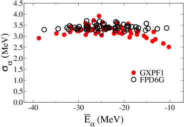
Figure 1: (Color online) Distribution of configuration in ⁴⁴Ti as function of the corresponding configurations centroids, in the pf-shell with interactions GXPF1 Honma et al. (2004) and FPD6G W. A. Richter, M. J. Van Der Merwe, R. R. Julies and B. A. Brown (1991); A. Poves, J. Sánchez-Solano, E. Caurier and F. Nowacki (2001)

While the configuration widths are constant for a given nuclide, they do depend on the nuclide in question. Table 1 shows the average configuration widths (and corresponding standard deviations) for a number of representative nuclides with valence particles in the $sd$-shell with the USD interaction Wildenthal (1984). The widths are largest for “half-filled” cases and for $N\sim Z$ nuclides. The scatter, as represented by the standard deviations, is nearly constant as well, except at nearly full or nearly empty spaces.

Table 1: Average configuration widths and corresponding standard deviations for several nuclides in the sd-shell with USD Wildenthal (1984) interaction.

Nuclide	$\langle\sigma_{\alpha}\rangle$ (MeV)	$\pm\Delta\sigma$ (MeV)
28Ne	4.84	1.17
28Na	6.68	0.84
28Mg	8.10	0.76
28Al	8.94	0.71
22Si	3.88	0.74
23Si	5.86	0.69
24Si	7.22	0.73
25Si	8.18	0.70
26Si	8.84	0.71
27Si	9.18	0.70
28Si	9.24	0.70
29Si	8.99	0.69
30Si	8.47	0.68
31Si	7.66	0.66
32Si	6.62	0.67
33Si	5.25	0.62
34Si	3.40	0.65

V.2 Distribution of configuration asymmetries

In Fig. 2 we plot the configuration asymmetry against the configuration centroid for two representative examples, ³³Ar in the $sd$-shell with the USD interaction (this is similar to Fig. 1 of Ref. V. K. B. Kota, V. Potbhare and P. Shenoy (1986), for 8 particles in the $sd$-shell, also showing rather strange gill-like structure), and ⁴⁴Ti in the $pf$-shell using GXPF1. Other nuclides in these spaces show the same generic behavior. The key results are, first, the range of the asymmetries, and second, the correlation of asymmetries with centroids. Please remember that here and throughout we consider scaled asymmetries and excesses, that is, normalized by the relevant configuration width.

The configuration asymmetries range from -2 to 2, which seems to be a general limit; in other sd- and pf-shell nuclei, we found only rare cases of $|m^{(3)}_{\alpha}|>2$ for $J$-summed moments ($J$-projected moments have wider ranges as we will see in a later section). It is important to keep in mind that these findings are only for complete $0\hbar\Omega$ spaces. We have not yet considered multi-shell configuration which may have a different range; such spaces are beyond the scope of our current methods and must be investigated in future.

The asymmetries are strongly correlated with the configuration centroids $\bar{E}_{\alpha}$: the most positive asymmetries are found at the most negative centroids and the the most negative asymmetries at the most positive centroids.

Following the discussion in III, we recomputed the asymmetries for “traceless” interactions (open squares) in Fig 2, that is, we subtract off the monopole potential. (In such a case the centroids all automatically go to zero, but we plot the asymmetries against the original centroids so one may see how the asymmetries are shifted.) Now most of the configuration asymmetries go to nearly zero. This supports the hypothesis that much of the configuration asymmetry derives mostly, although not completely, from Eq. (18).

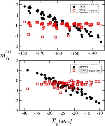
Figure 2: (Color online) Configuration asymmetries versus centroids for ³³Ar (top) and ⁴⁴Ti (bottom). Filled circles are for the full interaction; open squares have the monopole part of the interaction removed (“traceless”).

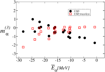
Figure 3: (Color online) Configuration asymmetries versus centroids for ²⁰Ne. Filled circles are for the full interaction; open squares have the monopole part of the interaction removed.

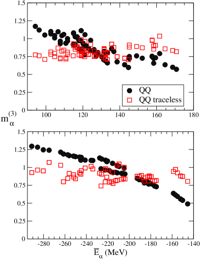
Figure 4: (Color online) Configuration asymmetries versus centroids for the collective $Q\cdot Q$ interactions for ³³Ar (top) and ⁴⁴Ti (bottom). Filled circles are for the full interaction; open squares have the monopole part of the interaction removed.

We considered a number of nuclides and interactions and found consistently the generic behavior illustrated in Fig. 2. There are two important variations. First, we refer the reader to Fig. 1 of Ref V. K. B. Kota, V. Potbhare and P. Shenoy (1986), which for 8 particles in the $sd$ shell has a range of asymmetries from 0.5 at low energies to -2 at high emergies. As another example, in Fig. 3 we show the distribution of configuration asymmetries for ²⁰Ne, using the USD interaction. Several of the asymmetries for low-lying configuration, in particular the lowest energy configuration, have asymmetries close to zero. While these are important exceptions to the examples in Fig. 2, the converse is also true: suggestions that asymmetries are small at low energies V. K. B. Kota, V. Potbhare and P. Shenoy (1986); Horoi et al. (2003) do not generalize.

For further investigation, in Fig. 3 we again consider the asymmetries for a traceless USD interaction in ²⁰Ne. Most of the asymmetries again go to zero, but the low-energy asymmetries that were near zero now become large and negative. We postulate that this arises from (probably attractive quadrupole) collectivity in the lowest states, which would lead to a large negative asymmetry. To test this idea we plot in Fig. 4 asymmetries for a pure (repulsive) $Q\cdot Q$ interaction, both with and without (“traceless”) the monopole-monopole interaction. In all our cases, including the two examples from the $sd$ shell (³³Ar, top) and $pf$ shell (⁴⁴Ti, bottom) we see strong asymmetries, even for the traceless interaction. In hindsight this is not surprising for a collective interaction, but supports our interpretation of the behavior of more realistic interactions in Figs. (2), (3). A realistic interaction has both attractive and repulsive collective pieces, e.g. $Q\cdot Q$ and $S\cdot S$, respectively, and in the bulk the collectivity tends to cancel, leading to traceless asymmetries near zero. At low energy, however, the attractive quadrupole collectivity dominates, pushing the asymmetry lower. This effect is smaller in the $pf$ shell, where a larger spin-orbit splitting weakens quadrupole collectivity V. G. Gueorguiev, J. P. Draayer, and C. W. Johnson (2001). To summarize, the behavior of the configuration asymmetries and any correlation with the configuration centroids result from an interplay between collective interactions and the monopole-monopole interaction.

V.3 Correlation of asymmetry and excess

We now turn to look at the relationship between the third and the fourth moments. Figure 1 of Ref. V. K. B. Kota, V. Potbhare and P. Shenoy (1986) indirectly suggest a correlation but those authors did not comment on it. Fig. 5 plots $(m^{(3)}_{\alpha})^{2}$ versus $m^{(4)}_{\alpha}$ for two nuclides in the $sd$-shell valence space, ²⁰Ne and ³³Ar. The observed linear correlation occurs in all other nuclides we considered as well, and Table 2 gives the slope and intercept (as well as the corresponding “uncertainties,” which are the diagonal correlation coefficients) for several $sd$-shell nuclides, all with the USD interactionWildenthal (1984). Table 3 shows slope, intercept, and uncertainties for a single nuclide in the $pf$-shell, ⁴⁴Ti, but for a variety of interactions, including quadrupole-quadrupole and a member of the two-body random ensemble (TBRE). There is a weak but statistically significant (the differences are several standard deviations) dependence on interaction and nuclide.

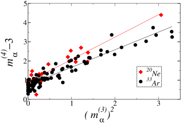
Figure 5: (Color online) Correlation between configuration asymmetries and excess in $sd$-shell nuclides ²⁰Ne and ³³Ar. Straight lines are least-squares linear fit.

Table 2: Intercept, slope, and respective standard deviations ($\sigma_{a}$, $\sigma_{b}$) corresponding to linear fits of $m_{4}$ vs. $m_{3}^{2}$ plots for different nuclides in the $sd$-shell valence space, with the USD interaction Wildenthal (1984).

Nuclide	intercept	slope	$\sigma_{\mathrm{intercept}}$	$\sigma_{\mathrm{slope}}$
20Ne	0.90	1.16	0.066	0.080
22Na	0.49	0.97	0.023	0.047
34Cl	0.86	0.97	0.032	0.037
33Ar	0.75	0.92	0.036	0.033

Table 3: Same as Table 2 but for different interactions on pf-shell ⁴⁴Ti.

Interaction	intercept	slope	$\sigma_{\mathrm{intercept}}$	$\sigma_{\mathrm{slope}}$
GXPF1	1.35	1.37	0.052	0.038
FPD6G	1.97	1.14	0.055	0.038
KB3G	2.30	1.17	0.090	0.032
$Q\cdot Q$	-0.25	1.60	0.031	0.037
TBRE	-0.70	1.88	0.029	0.085

We attribute the relation between $m^{(3)}$ and $m^{(4)}$ to a maximum entropy principle. For convenience we took the distribution a modified Breit-Wigner,

$$\rho(E)=\rho_{0}\frac{(E-E_{\mathrm{min}})(E_{\mathrm{max}}-E)}{(E-E_{0})^{2}+W^{2}},$$ (19)

and can adjust the parameters to fix the moments. We chose the form (19) because it is positive definite on the interval $(E_{\mathrm{min}},E_{\mathrm{max}})$, and one can compute the moments analytically. (Some alternatives such as Gram-Charlier are not positive-definite; for yet other alternatives, such as Cornish-Fisher V. K. B. Kota, V. Potbhare and P. Shenoy (1986) and binomial Zuker (2001), in practice one must integrate numerically to get accurate moments at large asymmetries.) We then computed the entropy,

$$S=-\int_{E_{\mathrm{min}}}^{E_{\mathrm{max}}}\rho(E)\ln\rho(E)dE.$$ (20)

For fixed width and normalization, the maximum entropy describes a straight line in the $m^{(3)})^{2}$-$m^{(4)}$ plane–albeit with different parameters, a slope of 1.67 and an intercept of $m^{(4)}-3=-0.07$. Nonetheless, this simple model makes for a reasonable understanding of the correlation between the third and fourth moments.

V.4 Distribution of $J$-projected moments

Finally, we consider the behavior of $J$-projected moments. This is relevant because some authors advocate the use of symmetric (Gaussian) distributions for $J$-projected partial densities, eschewing moments higher than the width R. U. Haq and S. S. M. Wong (1979); M. R. Zirnbauer and D. M. Brink (1981); Horoi et al. (2003).

In Fig. 6 we plot $J$-projected moments for two representative configurations for ⁴⁴Ti using GXPF1. One configuration (the 100th partition, or P100) is nearly symmetric with $m_{3}=-0.12$, while the other (P079) has high asymmetry ($m_{3}$ = 1.02). The centroids are plotted relative to the corresponding $J$-summed centroid, for ease of comparison.

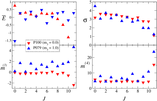
Figure 6: (Color online) Comparison of $J$-projected moments for ⁴⁴Ti for two configurations.

The moments are relatively constant, although with larger scatter; this not surprising because of the smaller dimensions, and the reader is cautioned not to overinterpret these graphs. (For partition 100, the total dimension is 784 levels, with 4 $J=0$ levels, 130 $J=6$ levels, and 25 $J=12$ levels; for partition 79, the total dimension is 1536 levels, 4 $J=0$ levels, 234 $J=6$ levels, and 23 $J=11$ levels.) The most significant trend is the width, which is largest for $J=0$ and shrinks almost monotonically. This was found in previous investigations for $J$-projected widths over the entire spaceJ.J.M. Verbaarschot and P.J. Brussaard (1982); J.N. Ginocchio and M.M. Yen (1975) and has been related to the predominance of $J=0$ ground states even with random two-body interactionsR. Bijker, A. Frank, and S. Pittel (1999); T. Papenbrock and H. A. Weidenmüller (2004). Similar behavior is found in other configurations in ⁴⁴Ti as well as in other nuclides.

In Fig. 7 we compare asymmetries versus centroids for both $J$-summed and $J$-projected moments (again for ⁴⁴Ti). The $J$-projected moments track the $J$-summed moments.

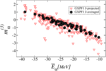
Figure 7: (Color online) Asymmetries versus centroids for ⁴⁴Ti in the pf-shell with interaction GXPF1 Honma et al. (2004). We compare $J$-summed asymmetries (filled circles) against $J$-projected (triangles).

Finally in Fig. 8 we consider the correlation of $m_{4}$ against $(m_{3})^{2}$ for both $J$-projected and $J$-summed moments (again for ⁴⁴Ti). Both show the same linear relation, although with slightly different slope and intercept. Also, the $J$-projected moments have a greater range.

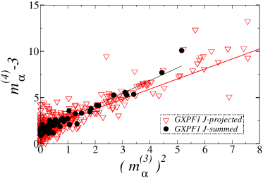
Figure 8: (Color online) Excess ($m_{4}$) plotted against the square of the asymmetry ($m_{3}$) for ⁴⁴Ti in the pf-shell with interaction GXPF1 Honma et al. (2004). We compare $J$-summed asymmetries (filled circles) against $J$-projected (triangles). Straight lines are least-squares linear fit.

VI Summary

We have investigated in detail the distribution of and correlations among configuration moments in $0\hbar\omega$ sd- and light pf-shell nuclei. We regained earlier results finding:

$\bullet$ the configuration widths are constant (but depend on the nuclide in question);

$\bullet$ $J$-projected widths are largest for smallest $J$ and decrease as $J$ increases; and

$\bullet$ the configuration asymmetry (third moment) is correlated with the configuration centroid (which, although documented before in the literature, had never been commented on).

We also found some new results, namely:

$\bullet$ the configuration asymmetries arise mostly, though not entirely, through the monopole part of the interaction; and

$\bullet$ the configuration excesses are linearly dependent upon the square of the asymmetry, which we attribute to a maximum entropy principle.

These last two are particularly interesting. They suggest that, if one wants to include the third and fourth moments, which are computationally intensive, one might be able to take a short cut and approximate the asymmetries from Eqn. (18) and the fourth moments from the linear relationship with the square of the asymmetry. Neither “universality” is absolute; intrinsic asymmetry (collectivity) at low energy must be considered to get correct asymmetries, and the slope and intercept of the $m^{(3)}$-$m^{(4)}$ relation depends weakly upon the interaction and nuclide. In the near future we plan to investigate in detail how much error is induced through such approximations and indeed if using the third and fourth moments do or do not improve descriptions of the density of states.

There is one final consequence of our work: if one is indeed to exploit knowledge of the asymmetry, any “model function” must be able to handle a range of at least $-2\leq m^{(3)}_{\alpha}\leq 2$. For example, binomial distributionsZuker (2001) fail to work over this entire range. We will address this issue in future work.

VII Acknowledgements

This work is supported by grant DE-FG52-03NA00082 from the Department of Energy /National Nuclear Security Agency. CWJ acknowledges helpful conversations with Dr. W. E. Ormand and Dr. J. Nabi.

References

- Hauser and Feshbach (1952) W. Hauser and H. Feshbach, Phys. Rev. 87, 366 (1952).
- T. Rauscher, F.-K. Thielemann and K.-L. Kratz (1997) T. Rauscher, F.-K. Thielemann and K.-L. Kratz, Phys. Rev. C 56, 1613 (1997).
- Bethe (1936) H. A. Bethe, Phys. Rev. 50, 332 (1936).
- Goriely (1996) S. Goriely, Nucl. Phys. A 605, 28 (1996).
- P. Demetriou and S. Goriely (2001) P. Demetriou and S. Goriely, Nucl. Phys. A 695, 95 (2001).
- B. A. Brown, A. Etchegoyen, and W. D. M. Rae (1984) B. A. Brown, A. Etchegoyen, and W. D. M. Rae (1984), OXBASH, the Oxford University-Buenos Aires-MSU shell model code, Michigan State University Cyclotron Laboratory Report No. 524.
- E. Caurier and F. Nowacki (1999) E. Caurier and F. Nowacki, Acta Phys. Pol. B 30, 705 (1999).
- (8) W. E. Ormand, REDSTICK shell model code, private communication.
- R.R. Whitehead, A. Watt, B.J. Cole, and I. Morrison (1977) R.R. Whitehead, A. Watt, B.J. Cole, and I. Morrison, Adv. Nucl. Phys. 9, 123 (1977).
- Ormand (1997) W. E. Ormand, Phys. Rev. C 56, R1678 (1997).
- Nakada and Alhassid (1997) H. Nakada and Y. Alhassid, Phys. Rev. Lett. 79, 2939 (1997).
- Nakada and Alhassid (1998) H. Nakada and Y. Alhassid, Phys. Lett. B 436, 231 (1998).
- J. B. French and K. F. Ratcliff (1971) J. B. French and K. F. Ratcliff, Phys. Rev. C 3, 94 (1971).
- S. Ayik and J.N. Ginocchio (1974) S. Ayik and J.N. Ginocchio, Nucl. Phys. A 221, 285 (1974).
- K. K. Mon and J. B. French (1975) K. K. Mon and J. B. French, Ann. Phys. 95, 90 (1975).
- Wong (1986) S. S. M. Wong, ed., Nuclear Statistical Spectroscopy (Oxford University Press, New York, 1986).
- Kota (1984) V. K. B. Kota, Z. Phys. A 315, 91 (1984).
- V. K. B. Kota, V. Potbhare and P. Shenoy (1986) V. K. B. Kota, V. Potbhare and P. Shenoy, Phys. Rev. C 34, 2330 (1986).
- Zuker (2001) A. P. Zuker, Phys. Rev. C 64, 021303 (2001).
- Horoi et al. (2003) M. Horoi, J. Kaiser, and V. Zelevinsky, Phys. Rev. C 67, 054309 (2003).
- Duflo and Zuker (1999) J. Duflo and A. P. Zuker, Phys. Rev. C 59, R2347 (1999).
- (22) E. Teran and C. W. Johnson, to be published.
- Wildenthal (1984) B. H. Wildenthal, Prog. Part. Nucl. Phys. 11, 5 (1984).
- Honma et al. (2004) M. Honma, T. Otsuka, B. A. Brown, and T. Mizusaki, Physical Review C 69, 034335 (2004).
- W. A. Richter, M. J. Van Der Merwe, R. R. Julies and B. A. Brown (1991) W. A. Richter, M. J. Van Der Merwe, R. R. Julies and B. A. Brown, Nucl. Phys. A 523, 325 (1991).
- A. Poves, J. Sánchez-Solano, E. Caurier and F. Nowacki (2001) A. Poves, J. Sánchez-Solano, E. Caurier and F. Nowacki, Nucl. Phys. A 694, 157 (2001).
- T.T.S. Kuo and G.E. Brown (1968) T.T.S. Kuo and G.E. Brown, Nucl. Phys. A 114, 241 (1968).
- A. Poves and A.P. Zuker (1981) A. Poves and A.P. Zuker, Phys. Rep. 70, 235 (1981).
- C. Jacquemin and S. Spitz (1979) C. Jacquemin and S. Spitz, J. Phys. G 5, L95 (1979).
- J.J.M. Verbaarschot and P.J. Brussaard (1982) J.J.M. Verbaarschot and P.J. Brussaard, Phys. Lett. B 102, 201 (1982).
- V. G. Gueorguiev, J. P. Draayer, and C. W. Johnson (2001) V. G. Gueorguiev, J. P. Draayer, and C. W. Johnson, Phys. Rev. C 63, 014318 (2001).
- R. U. Haq and S. S. M. Wong (1979) R. U. Haq and S. S. M. Wong, Nucl. Phys. A 327, 314 (1979).
- M. R. Zirnbauer and D. M. Brink (1981) M. R. Zirnbauer and D. M. Brink, Z. Phys. A 301, 237 (1981).
- J.N. Ginocchio and M.M. Yen (1975) J.N. Ginocchio and M.M. Yen, Nucl. Phys. A 239, 365 (1975).
- R. Bijker, A. Frank, and S. Pittel (1999) R. Bijker, A. Frank, and S. Pittel, Phys. Rev. C 60, 021302 (1999).
- T. Papenbrock and H. A. Weidenmüller (2004) T. Papenbrock and H. A. Weidenmüller, Phys. Rev. Lett. 93, 132503 (2004).