Exactly Solvable Model for the Decay of Superdeformed Nuclei

Abstract

The history and importance of superdeformation in nuclei is briefly discussed. A simple two-level model is then employed to obtain an elegant expression for the branching ratio for the decay via the E1 process in the normal-deformed band of superdeformed nuclei. From this expression, the spreading width $\Gamma^{\downarrow}$ for superdeformed decay is found to be determined completely by experimentally known quantities. The accuracy of the two-level approximation is verified by considering the effects of other normal-deformed states. Furthermore, by using a statistical model of the energy levels in the normal-deformed well, we can obtain a probabilistic expression for the tunneling matrix element $V$.

1 Superdeformed Nuclear Decay

Superdeformation is one of the most interesting examples of collective phenomena in atomic nuclei. Since its original experimental observation in 1986,[1] the properties of these high-spin rotational bands have fascinated experimentalists and theoreticians alike. When combined with precisely measured branching ratios and decay rates, a thorough theoretical understanding of the mechanism by which superdeformed (SD) nuclei are formed and then decay into normal-deformed (ND) bands promises to provide a window into nuclear structure unlike any other.

One of the major barriers to using SD decay to understand nuclear structure has been that there is no clear way to link the quantities measured in experiment directly with those which might shed light on the internal dynamics of the nucleus. Despite enormous strides made by experimentalists to measure observables precisely,[2, 3, 4] theorists have failed to reach a consensus on just what to do with these data. Ideally, we require a model which, while accounting for the rich physics of the SD nucleus, is also as simple as possible to allow for easy extraction of quantities of interest to theory.

The typical SD nuclear experiment[1, 2, 3, 4] creates nuclei in a high angular momentum state in the SD potential well. These nuclei then lose rotational energy by E2 transitions, eventually reaching a low enough angular momentum that it becomes energetically favorable to decay to states of the same angular momentum in the ND well. As each SD nucleus continues to decay, more strength moves into the energetically preferred ND band rather than continuing down the band of SD states. In practice, most of the decay-out of the SD band happens over the space of only two or three SD states, after which essentially all the strength has moved into the ND band. For a schematic diagram of this process, see Figure 1(a).

Figure 1: (a) Schematic diagram of the decay-out process. The SD band loses essentially all its strength to an ND band over the course of a few states. (b) The problem is commonly modeled with a double-well potential in deformation space. The shape of the potential is a function of the angular momentum of the nucleus.

It is customary to model the decay process as a double well problem, as in Figure 1(b). The nucleus is a quantum mechanical system moving in a spin-dependant potential in deformation space. The potential consists of two wells, and the eigenstates of each well in the absence of the other make up the pure SD and ND bands. In such models, it is the shape of the potential at various angular momenta which contains information about the underlying nuclear structure. Thus, an important goal for theories of this type is that they provide a method to relate the potential to experimental observables.

2 Two-State Model

The two-state model for SD nuclear decay [5] is an exactly solvable approximation to the decay-out scheme outlined in the previous section. The key assumption is that only one ND level participates significantly in the decay of a particular SD level of the same angular momentum. This reduces the problem to the familiar two-level mixing scenario of introductory quantum mechanics. The great advantage of this approach is that the two-state model rigorously yields simple formulae connecting experimental observations to the physics of the potential barrier.

Figure 2: Schematic diagram of the two-level model for SD nuclear decay. $\varepsilon_{S}$ and $\varepsilon_{N}$ are the energies of the unmixed SD and ND states, respectively; $\Gamma_{S}$ and $\Gamma_{N}$ are energy widths due to interaction with the electromagnetic field; and $V$ is the matrix element for tunneling through the barrier.

Keeping only the ND level of the same angular momentum nearest in energy to the decaying SD state, one can simplify the system to that shown in Figure 2. The dynamics of the model are thus completely determined by four parameters: the difference in the unmixed levels’ energies $\Delta=\varepsilon_{N}-\varepsilon_{S}$, the energy widths for coupling to the electromagnetic environment $\Gamma_{S}$ and $\Gamma_{N}$, and the tunneling matrix element $V$. A fifth parameter, the mean level spacing in the ND band $D_{N}$, can be taken as the unit of energy.

In the absence of the tunneling parameter $V$, the system reduces to two isolated Breit-Wigner resonances, and the retarded Green’s function in the energy domain is simply

$$G_{0}(E)=\left(\begin{array}[]{cc}\frac{1}{E+i\Gamma_{S}/2}&0\\ 0&\frac{1}{E-\Delta+i\Gamma_{N}/2}\end{array}\right)$$ (1)

in the $S,N$ basis. Coupling between the two levels is given by the simple perturbation matrix

$$\hat{V}=\left(\begin{array}[]{cc}0&V\\ V&0\\ \end{array}\right).$$ (2)

The full Green’s function is given exactly to all orders in $\hat{V}$ by Dyson’s Equation. Its inverse is

$$G^{-1}(E)=G_{0}^{-1}(E)-\hat{V}=\left(\begin{array}[]{cc}E+i\Gamma_{S}/2&-V\\ -V&E-\Delta+i\Gamma_{N}/2\end{array}\right).$$ (3)

The retarded Green’s function contains all information about the time evolution of the system. We are specifically interested in the branching ratios, which are given by Parseval’s Theorem to be

$$F_{i}=\Gamma_{i}\int^{\infty}_{-\infty}\frac{dE}{2\pi}|G_{iS}(E)|^{2},$$ (4)

where $i$ is either $S$ or $N$. The ND branching ratio follows:

$$F_{N}=\frac{\Gamma_{N}\Gamma^{\downarrow}/(\Gamma_{N}+\Gamma^{\downarrow})}{\Gamma_{S}+\Gamma_{N}\Gamma^{\downarrow}/(\Gamma_{N}+\Gamma^{\downarrow})},$$ (5)

a result we first noted in Ref. csb03. Here $\Gamma^{\downarrow}$ is the spreading width for tunneling through the barrier:

$$\Gamma^{\downarrow}=\frac{2\overline{\Gamma}V^{2}}{\Delta^{2}+\overline{\Gamma}^{2}},$$ (6)

where $\overline{\Gamma}\equiv\frac{\Gamma_{N}+\Gamma_{S}}{2}$.

In this case, Equation (6) is the exact result of Eq. (4), and it is also what one expects from correct application of Fermi’s Golden Rule.[5] We emphasize that, in general, $\Gamma^{\downarrow}\neq\langle\Gamma^{\downarrow}\rangle$, the ensemble average of $\Gamma^{\downarrow}$. In much previous literature (e.g., Ref. vigezzi), it was assumed that the two are equivalent, giving erroneous results. In fact, they are equal only in the continuum limit of overlapping resonances.[5] This is clearly not an appropriate approximation to most nuclei of interest, in which $D_{N}$ exceeds $\Gamma_{N}$ by several orders of magnitude. Indeed, in real nuclei the discrepancy between $\Gamma^{\downarrow}$ and its ensemble average can be as much as three to four orders of magnitude (see Table 1).

Values of $\Gamma^{\downarrow}$ and $\langle V\rangle$ for various SD decays in the $A\approx 150$ and $A\approx 190$ mass regions. $\langle\Gamma^{\downarrow}\rangle$ from Ref. lauritsen is tabulated for comparison. Values for $F_{N}$, $\Gamma_{S}$, $\Gamma_{N}$, and $D_{N}$ are also from Ref. lauritsen. $\Gamma^{\downarrow}$ is calculated from Eq. (7), either directly or, in the case of ${}^{152}\mathrm{Dy}(26)$, statistically, as discussed in the text, while $\langle V\rangle$ is given by Eq. (15). Angular momenta for the decaying SD states are given in parentheses. $F_{N}$ $\Gamma_{S}$ $\Gamma_{N}$ $D_{N}$ $\Gamma^{\downarrow}$ $\langle V\rangle$ $\langle\Gamma^{\downarrow}\rangle$ $=P_{out}$ (meV) (meV) (eV) (meV) (eV) (meV) ${}^{152}\mathrm{Dy}(28)$ 0.40 10.0 17 220 11 35 41 000 ${}^{152}\mathrm{Dy}(26)$ 0.81 7.0 17 194 78 87 220 000 ${}^{194}\mathrm{Hg}(12)$ 0.40 0.108 21 344 0.072 5.0 560 ${}^{194}\mathrm{Hg}(10)$ 0.97 0.046 20 493 1.6 35 37 000

Equation (5) demonstrates the power of using a simple, intuitively understandable model. We can instantly see that the result is correct, since it can be read as the branching ratio of a two-stage decay problem. That is, $F_{N}$ is the probability for the nucleus to tunnel through the barrier and then to decay down the ND band. Furthermore, it is eminently useful: we see that, given a set of experimental results, $\Gamma^{\downarrow}$ is known. Inverting Eq. (5) we find

$$\Gamma^{\downarrow}=\frac{F_{N}\Gamma_{N}\Gamma_{S}}{\Gamma_{N}-F_{N}(\Gamma_{N}+\Gamma_{S})},$$ (7)

so that the spreading width is fixed by experimental results. The recent work of Wilson and Davidson[8] has shown how to relate $\Gamma^{\downarrow}$ (Eq. (7)) to the barrier height by assuming it is equivalent to a fusion-like tunneling rate.

Since $\Gamma^{\downarrow}$ is a positive definite energy width, Eq. (7) implies a lower bound in the two-level model for the decay width due to E1 transitions in the ND band,

$$\Gamma_{N}>\frac{F_{N}\Gamma_{S}}{1-F_{N}}.$$ (8)

This prediction of the two-level model is especially significant due to the relatively high uncertainty in current values for $\Gamma_{N}$.

The estimated value[2] of $\Gamma_{N}$ for ${}^{152}\mathrm{Dy}(26)$ violates inequality (8). This could indicate a breakdown of the two-level approximation. However, such a conclusion would be precipitous due to the large uncertainty in the current best estimate of $\Gamma_{N}$, which could be off by a factor of two or more. An estimate of $\Gamma^{\downarrow}$ for this case can be obtained in the two-level model by cutting off the normal distribution for $\Gamma_{N}$ with inequality (8). The median value of $\Gamma^{\downarrow}$ so estimated is presented in Table 1, assuming the standard deviation $\sigma_{\Gamma_{N}}=\Gamma_{N}=17\mathrm{meV}$.

3 Gaussian Orthogonal Ensemble

We have seen that the two-level model gives an expression for the spreading width completely in terms of experimentally measurable quantities. Since $\Gamma^{\downarrow}$ is clearly related to the potential barrier between the two wells, this is a great stride toward the goal laid out in the first section, namely to find a simple relationship between observables and one or more parameters related directly to the shape of the potential.

The spreading or decay width $\Gamma^{\downarrow}$, however, is a rate, and less directly related to the shape of the potential than $V$, the tunneling matrix element itself. The problem in relating $V$ directly to experiment is clear from Eq. (6): we would need to know the value of $\Delta$, which is unfortunately not accessible with current experimental techniques. Lacking a complete solution of the nuclear structure problem, we derive a probabilistic theory for $V$, with its roots in the Gaussian Orthogonal Ensemble (GOE).

The GOE is a “structureless” assumption for the level distribution of the unmixed ND band, in which we assume only that the levels are eigenstates of some Hermitian Hamiltonian with time reversal and SO(3) symmetry. The states are characterized by the Wigner surmise,[9] a probability distribution for the spacing $sD_{N}$ between levels:

$$P(s)=\frac{\pi}{2}se^{-\pi s^{2}/4}.$$ (9)

Since we are interested in finding a probability distribution for unmixed levels, the SD and ND spectra are uncorrelated. Thus, given $s$, we have a rectangular probability density function for $\Delta$

$$\mathcal{P}_{s}(\Delta)=\frac{1}{sD_{N}}\Theta\left(\frac{s}{2}-\frac{|\Delta|}{D_{N}}\right).$$ (10)

The Heaviside step function $\Theta$ specifies that $\Delta$ is the detuning of the nearest neighbor.

Application of basic probability theory leads us to the density function for $\Delta$:

$$\mathcal{P}(\Delta)=\int_{0}^{\infty}\mathcal{P}_{s}(\Delta)P(s)ds=\frac{\pi}{2D_{N}}\mathrm{erfc}\left(\sqrt{\pi}\frac{|\Delta|}{D_{N}}\right).$$ (11)

Here $\mathrm{erfc}(x)$ is the complementary error function of $x$. The mean of this distribution is $D_{N}/4$.

From Eq. (6) we note that

$$|\Delta|=\sqrt{\frac{2\overline{\Gamma}}{\Gamma^{\downarrow}}\left(V^{2}-\frac{\Gamma^{\downarrow}\overline{\Gamma}}{2}\right)},$$ (12)

which implies

$$V\geq V_{min}=\sqrt{\frac{\Gamma^{\downarrow}\overline{\Gamma}}{2}}.$$ (13)

This allows calculation of the desired probability density function for $V$:

$$\mathcal{P}(V\geq V_{min})=2\mathcal{P}(\Delta)\left|\frac{d\Delta}{dV}\right|=\frac{2\overline{\Gamma}V\pi}{\Gamma^{\downarrow}|\Delta|D_{N}}\mathrm{erfc}\left(\sqrt{\pi}\frac{|\Delta|}{D_{N}}\right),$$ (14)

where $\Delta$ is given as a function of $V$ by Eq. (12).

We have arrived at a probability density function for $V$ solely in terms of experimentally measurable parameters. The mean of this distribution is

$$\langle V\rangle=\sqrt{\frac{\Gamma^{\downarrow}}{2\overline{\Gamma}}}\left[\frac{D_{N}}{4}+\mathcal{O}\left(\frac{\overline{\Gamma}^{2}}{D_{N}}\right)\right].$$ (15)

Values of $\langle V\rangle$ for specific SD decays are given in Table 1. In general, we can expect that $\langle V\rangle$ will be a typical value of $V$ for nuclei measured in the laboratory, since the standard deviation of the distribution (14) is comparable to the mean (15).

Equation (15) is a profound success of the two-level model. In fact, even by including more levels, a probabilistic statement like this represents the most information one can have about $V$ with the current types of experiments.

4 Beyond the Two-level Model

In the previous two sections, we solved an approximate model exactly. In reality, of course, the ND band is semi-infinite, starting at the bandhead and continuing upward. We now address the validity of the two-level approximation.

The simplest way to address this issue is to add a second ND level.[7] The branching ratio is now calculated in a three-dimensional Hilbert space, in exactly the same way as before. The inverse Green’s function is

$$G^{-1}(E)=\left(\begin{array}[]{ccc}E+i\Gamma_{S}/2&-V_{1}&-V_{2}\\ -V_{1}&E-\Delta_{1}+i\Gamma_{N}/2&0\\ -V_{2}&0&E-\Delta_{2}+i\Gamma_{N}/2\end{array}\right),$$ (16)

where the subscripts $1$ and $2$ pertain, respectively, to the nearest and next-nearest ND states to the decaying SD with the same angular momentum.

It is straightforward to obtain an analytic result for the three-level system by applying Eq. (4), but since we desire to know how changed the total branching ratios are from the two-state results over a range of parameters, it is perhaps more useful to calculate them numerically. Figure 3 shows the results for the $A\approx 190$ and $A\approx 150$ mass regions.

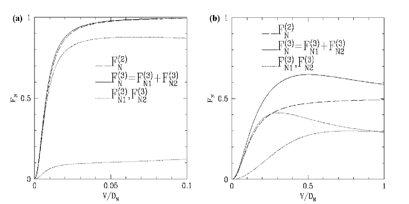
Figure 3: Numerical results comparing the two- and three-state total branching ratios. Superscripts indicate the model used whereas subscripts represent the nearest (1) and next-nearest (2) neighbor in the three-level case. (a) $A\approx 190$ mass region, as determined by $\Gamma_{S}/\Gamma_{N}=10^{-3}$. (b) $A\approx 150$ mass region with $\Gamma_{S}=\Gamma_{N}$. In both cases $\overline{\Gamma}/D_{N}=10^{-4}$. The levels were taken at their mean detunings within the GOE under the assumption that they lie on either side of the SD state, and in both cases $V_{1}=V_{2}=V$.

We note that the figure shows remarkably good agreement between the two- and three-level total branching ratios in the mass-190 region, particularly for values of $V$ that are likely according to Eq. (15). In the mass-150 region, as for ${}^{152}Dy$, they may disagree by as much as 25% ($I=28$) to 40% ($I=26$) due to the larger value of the coupling matrix element $V$ and the smaller level spacing, i. e., higher density of states. This supports the validity of the two-level approximation for the mass-190 region, in the sense that the addition of the third level has not affected the physically measured quantities too significantly. In the mass-150 region, the three-level approximation yields a significant correction to the two-state branching ratios for values of $V/D_{N}\gtrsim 0.15$.

Further support for the two-level approximation is given by Ref. dzyublik03, in which Dzyublik and Utyuzh exactly solve the problem in the approximation of an infinite (in both directions), equally spaced ND band. Their results also show remarkably strong agreement with the two-level approximation for typical values of $\Delta$.

5 Conclusions

Our three-state results, together with the results of Ref. dzyublik03, demonstrate that the two-state model is sufficient to describe the dominant decay-out process of SD nuclei. Within the two-state model, we have shown that the decay out of an SD level via the E1 process in the ND band is a two-step process, whose branching ratio (5) is expressed in terms of three measurable rates, $\Gamma_{S}$, $\Gamma_{N}$, and $\Gamma^{\downarrow}$. We have also shown how to determine the tunneling matrix element $V$ (Eqs. (14) and (15)) from the measured values of $\Gamma^{\downarrow}$ and a statistical model of the ND band. It is hoped that these results will help to clarify the nature of the decay-out process in SD nuclei, and that their elegance will inspire further promising studies such as Ref. wilson04.

References

- [1] P. J. Twin et al.,Phys. Rev. Lett. 57, 811 (1986).
- [2] T. Lauritsen et al., Phys. Rev. Lett. 88, 042501 (2002).
- [3] R. Krücken et al., Phys. Rev. C55, R1625 (1997).
- [4] A. N. Wilson et al., Phys. Rev. Lett. 90, 142501 (2003), and references therein.
- [5] C. A. Stafford and B. R. Barrett, Phys. Rev. C60, 51305 (1999).
- [6] E. Vigezzi, R. A. Broglia, and T. Døssing, Phys. Lett. B249, 163 (1990). E. Vigezzi, R. A. Broglia, and T. Døssing, Nucl. Phys. A520, 179c (1990).
- [7] D. M. Cardamone, C. A. Stafford, and B. R. Barrett, Phys. Rev. Lett. 91, 102502 (2003).
- [8] A. N. Wilson and P. M. Davidson, Phys. Rev. C69, 041303(R) (2004).
- [9] M. L. Mehta, Random Matrices (Academic Press, New York, 1991).
- [10] A. Ya. Dzyublik and V. V. Utyuzh, Phys. Rev. C68, 024311 (2003).