Hartree-Fock-Bogolyubov calculations with Gaussian expansion method

We extensively develop an algorithm of implementing the Hartree-Fock-Bogolyubov calculations, in which the Gaussian expansion method is employed. This algorithm is advantageous in describing the energy-dependent exponential and oscillatory asymptotics of the quasiparticle wave functions at large $r$, and in handling various effective interactions including those with finite ranges. We apply the present method to the oxygen isotopes with the Gogny interaction, keeping the spherical symmetry. In respect to the new magic numbers, effects of the pair correlation on the $N=16$ and $32$ nuclei are investigated.

PACS numbers: 21.60.Jz, 21.30.Fe, 21.10.Gv, 21.10.Pc

Keywords: Hartree-Fock-Bogolyubov calculation, Gaussian expansion method, new magic numbers, finite-range interaction, wave-function asymptotics

1 Introduction

Experimental data using the radioactive beams have disclosed exotic natures of atomic nuclei far from the $\beta$-stability. Some of the data cast questions on the conventional nuclear structure theories, which have been founded mainly on top of the data along the $\beta$-stability line. Density profile of nuclei near the proton or neutron drip-line is remarkably different from that of the stable nuclei, sometimes making halos [1]. Furthermore, new magic numbers, e.g. $N=16$ and $32$, have been reported in the region off the $\beta$-stability line [2]. A property of the effective interaction, which has not been investigated sufficiently, seems to play a role in the variation of magic numbers [3, 4].

The mean-field theories provide us with a good first approximation for bound states of nuclei. The Hartree-Fock (HF) theory, through which we can construct the nuclear mean-field in a self-consistent manner, is a desirable tool to obtain the single-particle (s.p.) orbits of nuclei from microscopic standpoints. In addition, the HF theory is useful in investigating basic and global natures of effective interactions. However, the pair correlation between identical nucleons yields a significant correction to the HF approximation. The pair correlation, which gives rise to the superfluidity, can be treated self-consistently in the Hartree-Fock-Bogolyubov (HFB) theory [5]. For nuclei in the vicinity of the drip line, appropriate treatment of the wave-function asymptotics at large $r$ may be important, as has been shown in the HF framework [6]. If the pairing is taken into consideration, the s.p. levels that are far below the Fermi energy in the HF scheme couple to the continuum. In applying the HFB approximation to nuclei near the drip line, we need a method capable of handling the wave-function asymptotics for bound nucleons and those for nucleons in the continuum simultaneously. While this point has been argued in association with the zero-range Skyrme interaction [7], it has not been considered sufficiently for finite-range interactions, primarily because no efficient methods to treat the wave-function asymptotics have been known in the case that the non-local nuclear currents are required.

We recently proposed a new computational method [6] to implement the HF calculations, by extensively applying the Gaussian expansion method (GEM) [8]. It was demonstrated that the energy-dependent exponential asymptotics of wave functions are handled efficiently, even with finite-range interactions. In this article we further extend the method to the HFB calculations. Both the exponential and the oscillatory asymptotics can be practically represented in a single set of Gaussian bases. This method is easily adaptable to calculations with finite-range interactions, and therefore will be useful in studying effective interactions to describe nuclear properties including the pair correlation. The present method is applied to the oxygen isotopes in practice, keeping the spherical symmetry. The interaction-dependence of the shell structure near $N=16$ and $32$ is also investigated, in the light of the pair correlation.

2 Single-particle bases and HFB equation

In this paper we assume the mean fields to be spherically symmetric and to preserve the parity. Though almost straightforward, extension to the deformed cases will be left as a future study.

To represent the s.p. wave functions, we introduce bases having the following form:

$$\varphi_{\nu\ell jm}({\mathbf{r}}) = R_{\nu\ell j}(r)\,[Y^{(\ell)}(\hat{\mathbf{r}})\chi_{\sigma}]^{(j)}_{m}\,;$$

$$R_{\nu\ell j}(r) = \mathcal{N}_{\nu\ell j}\,r^{\ell}\exp(-\nu r^{2})\,.$$ (1)

Here $Y^{(\ell)}(\hat{\mathbf{r}})$ expresses the spherical harmonics and $\chi_{\sigma}$ the spin wave function. We drop the isospin index without confusion. The index $\nu$ corresponds to the range parameter of the Gaussian basis. We allow the range parameter $\nu$ to be complex [9], and hereafter denote $\textrm{Re}(\nu)$ and $\textrm{Im}(\nu)$ by $\nu_{\mathrm{r}}$ and $\nu_{\mathrm{i}}$, respectively. Note that $\nu_{\mathrm{r}}>0$. The constant $\mathcal{N}_{\nu\ell j}$ is determined by

$$\mathcal{N}_{\nu\ell j}=\frac{2^{\ell+\frac{7}{4}}}{\pi^{\frac{1}{4}}\sqrt{(2\ell+1)!!}}\,\,\nu_{\mathrm{r}}^{\frac{2\ell+3}{4}},$$ (2)

so as for $\langle\varphi_{\nu\ell jm}|\varphi_{\nu\ell jm}\rangle$ to be unity. The bases of Eq. (1) with different $\nu$’s are not orthogonal to one another. The norm matrix for each $(\ell,j)$ is composed of the elements of

$$N^{(\ell j)}_{\nu\nu^{\prime}}=\langle\varphi_{\nu\ell jm}|\varphi_{\nu^{\prime}\ell jm}\rangle=\left(\frac{2\sqrt{\nu_{\mathrm{r}}\nu^{\prime}_{\mathrm{r}}}}{\nu^{\ast}+\nu^{\prime}}\right)^{\ell+\frac{3}{2}}\,.$$ (3)

In the GEM we take $\nu$’s belonging to a geometric progression. The GEM basis-set with real $\nu$’s has been shown to work efficiently in the HF calculations [6] as well as in solving few-body problems [10], including the cases of loosely bound systems. The exponential decrease of density at large $r$ is described to a good approximation by a superposition of the Gaussians with various ranges. For a complex $\nu$, the linear combinations of $R_{\nu\ell j}$ and $R_{\nu^{\ast}\ell j}$ clarify the oscillating structure as

$$[R_{\nu\ell j}(r)+R_{\nu^{\ast}\ell j}(r)]/2 = \mathcal{N}_{\nu\ell j}\,r^{\ell}\exp(-\nu_{\mathrm{r}}r^{2})\,\cos(\nu_{\mathrm{i}}r^{2})\,,$$

$$~{}[R_{\nu\ell j}(r)-R_{\nu^{\ast}\ell j}(r)]/2i = \mathcal{N}_{\nu\ell j}\,r^{\ell}\exp(-\nu_{\mathrm{r}}r^{2})\,\sin(\nu_{\mathrm{i}}r^{2})\,.$$ (4)

Indeed, by superposing the complex-range Gaussian bases, oscillating behavior of the wave functions in the scattering states as well as in the states with high-nodal wave functions can be expressed efficiently [9].

To formulate the HFB theory for non-orthogonal bases, we consider the creation (annihilation) operator $c_{\nu\ell jm}^{\dagger}$ ($c_{\nu\ell jm}$), which is associated with $\varphi_{\nu\ell jm}$ and obeys the non-canonical commutation relations,

$$\{c_{\nu\ell jm},c_{\nu^{\prime}\ell^{\prime}j^{\prime}m^{\prime}}^{\dagger}\}=\delta_{\ell\ell^{\prime}}\delta_{jj^{\prime}}\delta_{mm^{\prime}}N^{(\ell j)}_{\nu\nu^{\prime}}\,,\quad\{c_{\nu\ell jm},c_{\nu^{\prime}\ell^{\prime}j^{\prime}m^{\prime}}\}=\{c_{\nu\ell jm}^{\dagger},c_{\nu^{\prime}\ell^{\prime}j^{\prime}m^{\prime}}^{\dagger}\}=0\,.$$ (5)

The HFB equation for non-orthogonal bases is derived generally in Appendix A, and it is reduced to the equation with the $\ell$ and $j$ conservation in Appendix B. Under the spherical symmetry, which implies that $\ell$ and $j$ as well as $m$ are conserved, the generalized Bogolyubov transformation is written as

$$\alpha_{n\ell jm}^{\dagger}=\sum_{\nu}\left[U^{(\ell j)}_{\nu n}c_{\nu\ell jm}^{\dagger}+V^{(\ell j)}_{\nu n}c_{\nu\overline{\ell jm}}\right]\,,$$ (6)

where the s.p. state $(\nu\overline{\ell jm})$ stands for the time reversal to $(\nu\ell jm)$. The solution of the HFB equation (41) gives the quasiparticle (q.p.) state represented by $(n\ell jm)$, whose eigenvalue, $\epsilon_{n\ell j}$, is called quasiparticle energy. In $Z$ or $N=\mathrm{odd}$ nuclei, we should replace $(\mathsf{U}^{(\ell j)},-\mathsf{V}^{(\ell j)})$ by $(\mathsf{V}^{(\ell j)\ast},\mathsf{U}^{(\ell j)\ast})$ in Eq. (39) for a nucleon which has the lowest $\epsilon_{n\ell j}$. With the spherical symmetry, this implies addition of $\frac{1}{2j+1}(U^{(\ell j)}_{\nu n}U^{(\ell j)^{\ast}}_{\nu^{\prime}n}-V^{(\ell j)\ast}_{\nu n}V^{(\ell j)}_{\nu^{\prime}n})$ to $\rho^{(\ell j)}_{\nu\nu^{\prime}}$ and $-\frac{1}{2j+1}(U^{(\ell j)}_{\nu n}V^{(\ell j)^{\ast}}_{\nu^{\prime}n}+V^{(\ell j)\ast}_{\nu n}U^{(\ell j)}_{\nu^{\prime}n})$ to $\kappa^{(\ell j)}_{\nu\nu^{\prime}}$ in Eq. (39). With this modification, the form of the HFB equation (41) does not change. If we use the linear combination of Eq. (4) instead of the complex-range Gaussian bases, all matrices in Eq. (41) can be taken to be real.

3 Asymptotic behavior of quasiparticle wave functions

We next consider the asymptotic behavior of the q.p. wave functions at large $r$. The HFB equation (41) is easily represented in terms of the radial coordinate $r$, by converting the label of the basis $\nu$ to $r$. For the time being we consider the HFB equation for neutrons. At sufficiently large $r$, the nuclear force becomes negligible, and the following asymptotic equations are derived [11],

$$\left(-\frac{1}{2M}\frac{d^{2}}{dr^{2}}-\lambda\right)\,[r\,U^{(\ell j)}_{n}(r)] \approx \epsilon_{n\ell j}[r\,U^{(\ell j)}_{n}(r)]\,,$$

$$\left(-\frac{1}{2M}\frac{d^{2}}{dr^{2}}-\lambda\right)\,[r\,V^{(\ell j)}_{n}(r)] \approx -\epsilon_{n\ell j}[r\,V^{(\ell j)}_{n}(r)]\,.$$ (7)

As long as the nucleus is bound, the chemical potential $\lambda$ should be negative. Since we take $\epsilon_{n\ell j}$ to be positive, Eq. (7) derives the asymptotic form,

$$r\,V^{(\ell j)}_{n}(r)\approx\exp(-\eta^{(\ell j)}_{n+}r)\,,\quad r\,U^{(\ell j)}_{n}(r)\approx\left\{\begin{array}[]{ccc}\exp(-\eta^{(\ell j)}_{n-}r)&\mbox{for}&\lambda+\epsilon_{n\ell j}<0\\ \cos(p^{(\ell j)}_{n}r+\theta^{(\ell j)}_{n})&\mbox{for}&\lambda+\epsilon_{n\ell j}>0\end{array}\right.,$$ (8)

where $\eta^{(\ell j)}_{n\pm}=\sqrt{2M(-\lambda\pm\epsilon_{n\ell j})}$, $p^{(\ell j)}_{n}=\sqrt{2M(\lambda+\epsilon_{n\ell j})}$ and $\theta^{(\ell j)}_{n}$ is an appropriate real number. Note that $\eta^{(\ell j)}_{n+}>\eta^{(\ell j)}_{n-}$. Corresponding to the asymptotic behavior of $U^{(\ell j)}_{n}(r)$, the q.p. energies are discrete only for $0\leq\epsilon_{n\ell j}<-\lambda$. Thus the deeply bound s.p. states in the HF approximation are embedded in the continuum in the HFB theory. It is now obvious that, in the HFB calculations, we have to treat both the exponential and the oscillatory asymptotics which depend on the q.p. energy. In Ref. [7], these asymptotics are handled by adopting the transformed harmonic oscillator (THO) bases. However, it is not easy to apply the THO bases if the non-local currents are required, as in the case of the finite-range interactions. As will be demonstrated in Sec. 5, the GEM provides a practical method in handling the energy-dependent asymptotics even in the presence of the non-local currents.

The asymptotic behavior of the neutron density and pair current [12] is derived from Eq. (8). The density matrix and the pairing tensor in Eq. (39) are converted to the $r$-representation as

$$\rho^{(\ell j)}(r,r^{\prime}) = \sum_{n}V^{(\ell j)\ast}_{n}(r)\,V^{(\ell j)}_{n}(r^{\prime})\,,$$

$$\kappa^{(\ell j)}(r,r^{\prime}) = \sum_{n}V^{(\ell j)\ast}_{n}(r)\,U^{(\ell j)}_{n}(r^{\prime})\,,$$ (9)

for $N=\mathrm{even}$ nuclei. The density and the pair current are then defined by

$$\rho(r) = \sum_{\ell j}(2j+1)\,\rho^{(\ell j)}(r,r)\,,$$

$$\kappa(r) = \sum_{\ell j}(2j+1)\,\kappa^{(\ell j)}(r,r)\,.$$ (10)

Denoting the smallest q.p. energy by $\epsilon_{\mathrm{min}}$, we immediately obtain the asymptotic form of $\rho(r)$ as

$$r^{2}\rho(r)\approx\exp(-2\eta^{\mathrm{min}}_{+}r)\,,$$ (11)

where $\eta^{\mathrm{min}}_{+}=\sqrt{2M(-\lambda+\epsilon_{\mathrm{min}})}$. In order for an $N=\mathrm{odd}$ nucleus to be bound, the condition $\lambda+\epsilon_{\mathrm{min}}<0$ must be fulfilled, because $V^{(\ell j)}_{n}(r)$ is replaced by $U^{(\ell j)}_{n}(r)$ for the last neutron. The contribution of the last neutron yields the asymptotic form

$$r^{2}\rho(r)\approx\exp(-2\eta^{\mathrm{min}}_{-}r)\,,$$ (12)

which damps more slowly than the form in Eq. (11).

As pointed out in Ref. [12], a complication may arise in the close vicinity of the drip line. If $-\lambda$ is almost vanishing and no q.p. level satisfies $\lambda+\epsilon_{n\ell j}<0$, it is difficult to draw definite conclusion on the asymptotic behavior of $\rho(r)$. For $N=\mathrm{even}$ nuclei, arguments based on the q.p. energy suggest that the component of $\lambda+\epsilon_{n\ell j}\rightarrow+0$ becomes dominant at the $r\rightarrow\infty$ limit, giving the asymptotics of $r^{2}\,\rho(r)\approx\exp\!\left[-2\sqrt{4M(-\lambda)}\,r\right]$. However, the spectroscopic amplitude of this component may be negligibly small in the physically interesting region. The actual situation is in the balance between the damping factor and the spectroscopic amplitude of the q.p. levels near $-\lambda$. Moreover, because of this subtlety, in practical calculations the asymptotic behavior of $\rho(r)$ could be sensitive to the details of the method, even if individual q.p. wave function has the asymptotics consistent with its q.p. energy. Even with the high adaptability of the GEM to the wave-function asymptotics at large $r$, it is beyond scope of the present study to obtain reliable asymptotics of $\rho(r)$ for nuclei with $\lambda+\epsilon_{\mathrm{min}}>0$. Similar arguments apply to $N=\mathrm{odd}$ nuclei.

The asymptotics for $\kappa(r)$ could also be complicated. We separately consider contribution of the discrete q.p. states and that of the q.p. continuum. The discrete q.p. states, which satisfy $\lambda+\epsilon_{n\ell j}<0$, contribute to $\kappa(r)$ asymptotically with the damping factor $\exp\!\left[-(\eta^{(\ell j)}_{n+}+\eta^{(\ell j)}_{n-})r\right]$. Because $\eta^{(\ell j)}_{n+}+\eta^{(\ell j)}_{n-}$ is a decreasing function of $\epsilon_{n\ell j}$ for a fixed $\lambda$, the q.p. level just below $-\lambda$ dominates over the other discrete states at large $r$. The damping factor becomes $\exp\!\left[-2\sqrt{4M(-\lambda)}\,r\right]$ at the $\lambda+\epsilon_{n\ell j}\rightarrow-0$ limit. In the states having $\lambda+\epsilon_{n\ell j}>0$, we have a damping factor $\exp(-\eta^{(\ell j)}_{n+}r)$, which is multiplied by the oscillating factor $\cos(p^{(\ell j)}_{n}r+\theta^{(\ell j)}_{n})$, at large $r$. Hence the q.p. level closest to $-\lambda$ has dominant contribution to $\kappa(r)$ at the $r\rightarrow\infty$ limit. The component of $\lambda+\epsilon_{n\ell j}\rightarrow+0$ gives the most slowly damping factor $\exp\!\left[-\sqrt{4M(-\lambda)}\,r\right]$. However, similarly to $\rho(r)$ in the $\lambda\approx 0$ case, spectroscopic amplitudes of the q.p. levels become relevant. This complicates description of the asymptotic behavior of $\kappa(r)$ near the neutron drip line.

For proton wave functions, the Coulomb interaction influences the wave functions at large $r$, although it does not affect the criterion whether or not individual q.p. levels are discrete. The above arguments for the neutron functions can be applied if the asymptotic forms are properly modified. Nevertheless, the complication near the drip line is expected to be less serious than for neutron wave functions, owing to the presence of the Coulomb barrier.

4 Effective interaction

We shall consider the effective Hamiltonian comprised of the kinetic energy and the effective two-body interaction,

$$\hat{H}=\hat{K}+\hat{V}\,;\quad\hat{K}=\sum_{i}\frac{\mathbf{p}_{i}^{2}}{2M}\,,\quad\hat{V}=\sum_{i<j}v_{ij}\,.$$ (13)

Here $i$ and $j$ are the indices of each nucleon. The s.p. matrix element of the kinetic term is calculated as

$$\langle\varphi_{\nu\ell jm}|\frac{\mathbf{p}^{2}}{2M}|\varphi_{\nu^{\prime}\ell jm}\rangle=\frac{2\ell+3}{2M}\cdot\frac{2\nu^{\ast}\nu^{\prime}}{\nu^{\ast}+\nu^{\prime}}\,N^{(\ell j)}_{\nu\nu^{\prime}}\,.$$ (14)

As in Refs. [4, 6], the effective interaction $v_{ij}$ is assumed to have the following form,

$$v_{12} = v_{12}^{(\mathrm{C})}+v_{12}^{(\mathrm{LS})}+v_{12}^{(\mathrm{TN})}+v_{12}^{(\mathrm{DD})}\,;$$

$$v_{12}^{(\mathrm{C})} = \sum_{\mu}(t_{\mu}^{(\mathrm{SE})}P_{\mathrm{SE}}+t_{\mu}^{(\mathrm{TE})}P_{\mathrm{TE}}+t_{\mu}^{(\mathrm{SO})}P_{\mathrm{SO}}+t_{\mu}^{(\mathrm{TO})}P_{\mathrm{TO}})f_{\mu}^{(\mathrm{C})}(r_{12})\,,$$

$$v_{12}^{(\mathrm{LS})} = \sum_{\mu}(t_{\mu}^{(\mathrm{LSE})}P_{\mathrm{TE}}+t_{\mu}^{(\mathrm{LSO})}P_{\mathrm{TO}})f_{\mu}^{(\mathrm{LS})}(r_{12})\,\mathbf{L}_{12}\cdot(\mathbf{s}_{1}+\mathbf{s}_{2})\,,$$

$$v_{12}^{(\mathrm{TN})} = \sum_{\mu}(t_{\mu}^{(\mathrm{TNE})}P_{\mathrm{TE}}+t_{\mu}^{(\mathrm{TNO})}P_{\mathrm{TO}})f_{\mu}^{(\mathrm{TN})}(r_{12})\,r_{12}^{2}S_{12}\,,$$

$$v_{12}^{(\mathrm{DD})} = t_{3}(1+x_{3}P_{\sigma})[\rho(\mathbf{r}_{1})]^{\alpha}\delta(\mathbf{r}_{12})\,,$$ (15)

where $\mathbf{r}_{12}=\mathbf{r}_{1}-\mathbf{r}_{2}$, $r_{12}=|\mathbf{r}_{12}|$, $\mathbf{p}_{12}=(\mathbf{p}_{1}-\mathbf{p}_{2})/2$, $\mathbf{L}_{12}=\mathbf{r}_{12}\times\mathbf{p}_{12}$, $\mathbf{s}_{i}$ is the nucleon spin operator, and $S_{12}$ is the tensor operator $S_{12}=4\,[3(\mathbf{s}_{1}\cdot\hat{\mathbf{r}}_{12})(\mathbf{s}_{2}\cdot\hat{\mathbf{r}}_{12})-\mathbf{s}_{1}\cdot\mathbf{s}_{2}]$. The projectors $P_{\mathrm{SE}}$, $P_{\mathrm{TE}}$, $P_{\mathrm{SO}}$ and $P_{\mathrm{TO}}$ are expressed as

$$P_{\mathrm{SE}}=\frac{1-P_{\sigma}}{2}\,\frac{1+P_{\tau}}{2}\,, P_{\mathrm{TE}}=\frac{1+P_{\sigma}}{2}\,\frac{1-P_{\tau}}{2}\,,$$

$$P_{\mathrm{SO}}=\frac{1-P_{\sigma}}{2}\,\frac{1-P_{\tau}}{2}\,, P_{\mathrm{TO}}=\frac{1+P_{\sigma}}{2}\,\frac{1+P_{\tau}}{2}\,,$$ (16)

in terms of the spin and isospin exchange operators $P_{\sigma}$, $P_{\tau}$. In Eq. (15), $f_{\mu}$ represents an appropriate function, $\mu$ stands for the parameter attached to the function, and $t_{\mu}$ the coefficient. By taking various functions for $f_{\mu}$, Eq. (15) covers a wide variety of effective interactions. The Gogny interaction [13] is obtained by setting $f_{\mu}^{(\mathrm{C})}(r_{12})=\exp(-\mu r_{12}^{2})$, $f^{(\mathrm{LS})}(r_{12})=\nabla^{2}\delta(\mathbf{r}_{12})$ and $v_{12}^{(\mathrm{TN})}=0$. In Ref. [4] we have developed M3Y-type interactions, in which we take $f_{\mu}^{(\mathrm{C,LS,TN})}(r_{12})=\exp(-\mu r_{12})/\mu r_{12}$.

The matrix elements of $v_{12}^{(\mathrm{C,LS,TN})}$ can be calculated by utilizing the Fourier transformation of $f_{\mu}(r_{12})$ [6]. Most formulae in Ref. [6] are straightforwardly applicable, although the complex-range Gaussian bases lead to a slight modification in the radial integral (Eqs. (24–26) in Ref. [6]):

$$\int_{0}^{\infty}r^{2}drj_{\lambda}(kr)R_{\nu^{\ast}\ell j}(r)R_{\nu^{\prime}\ell^{\prime}j^{\prime}}(r)\hskip 227.62204pt$$

$$=\frac{\displaystyle 2^{\frac{\ell+\ell^{\prime}}{2}}\,\left(\frac{\ell+\ell^{\prime}-\lambda}{2}\right)!}{\sqrt{(2\ell+1)!!(2\ell^{\prime}+1)!!}}\,\frac{\sqrt{2\nu_{\mathrm{r}}}^{\ell+\frac{3}{2}}\sqrt{2\nu^{\prime}_{\mathrm{r}}}^{\ell^{\prime}+\frac{3}{2}}}{(\nu^{\ast}+\nu^{\prime})^{\frac{\ell+\ell^{\prime}+3}{2}}}\cdot Q_{\nu^{\ast}\nu^{\prime}}^{\lambda}\,L^{(\lambda+\frac{1}{2})}_{\frac{\ell+\ell^{\prime}-\lambda}{2}}(Q_{\nu^{\ast}\nu^{\prime}}^{2})\,\exp(-Q_{\nu^{\ast}\nu^{\prime}}^{2})\,,$$ (17)

where $L^{(\alpha)}_{n}(x)$ is the associated Laguerre polynomial and

$$Q_{\nu^{\ast}\nu^{\prime}}=\frac{k}{2(\nu^{\ast}+\nu^{\prime})^{\frac{1}{2}}}\,.$$ (18)

We need only the $\ell+\ell^{\prime}+\lambda=\mathrm{even}$ cases for the integral of Eq. (17). In coding a computer program, we prepare a subprogram for the $k$-integration (see Eq. (28) of Ref. [6]), which is the only part dependent on the form of $f_{\mu}(r_{12})$. This allows us to handle various interaction forms only by substituting the subprogram. Although analytic formulae for the $k$-integration were given in Ref. [6], their application sometimes causes serious round-off errors. Numerical integration over $k$ is recommended to reduce the errors.

Mean-field approaches for nuclei are sometimes discussed in connection to the density-functional theory (DFT). Although the DFT is a rigorous theory, we have to know a good density-functional form of energy for practical applications. The most popular density-functional form in nuclear structure physics is based on the Skyrme interaction and its extensions, whose parameters are adjusted to the known data. Some of the Skyrme density functionals involve currents that cannot be derived from two-body interactions. Still the form of the Skyrme density functionals is quite restricted, since all currents are assumed to be local. In order to know appropriate form of density functional for nuclei covering large area of the nuclear chart, it will be an important step to explore finite-range effective two-body interactions. It is noted that, whereas we consider two-body interactions having the form of Eq. (15) in this paper, the GEM algorithm is applicable also to the DFT, which may not necessarily be connected to two-body interactions.

Once storing the interaction matrix elements and having a trial set of $U^{(\ell j)}_{\nu n}$ and $V^{(\ell j)}_{\nu n}$, we obtain the HFB equation (41) with $h^{(\ell j)}_{\nu\nu^{\prime}}$ and $\Delta^{(\ell j)}_{\nu\nu^{\prime}}$ defined in Eqs. (30) and (40), and the equation is solved iteratively until convergence.

5 Numerical examples

We now apply the present method of the HFB calculations to several nuclei, assuming the spherical symmetry and the parity conservation. The center-of-mass energy is fully removed before variation, by subtracting both the one-body and two-body terms from the Hamiltonian of Eq. (13).

5.1 Application to oxygen isotopes with Gogny interaction

We first show results for oxygen isotopes, using the standard D1S parameter-set [14] of the Gogny interaction. While the real-range GEM basis-sets are efficient to describe nodeless but broadly distributing wave functions, the complex-range GEM sets seem suitable for reproducing the oscillating behavior required in reaction studies [9]. In the HFB calculations both types of wave functions come into the problem. We try the following three basis-sets, a set comprised of real-range bases, a set of complex-range bases and a set of their mixture;

$$\begin{array}[]{lllll}\mbox{Set~{}A\,:}&\nu_{\mathrm{r}}=\nu_{\omega}\,b^{-2\alpha}\,,&b=1.20\,,&\,\nu_{\mathrm{i}}=0\,,&(\alpha=-2,-1,0,\cdots,K-3)\,;\\ \mbox{Set~{}B\,:}&\nu_{\mathrm{r}}=\nu_{\omega}\,b^{-2\alpha}\,,&b=1.15\,,&\,{\displaystyle\frac{\nu_{\mathrm{i}}}{\nu_{\mathrm{r}}}=\pm\frac{\pi}{2}}\cdot 0.6\,,&(\alpha=0,1,\cdots,K/2-1)\,;\vspace*{2mm}\\ \mbox{Set~{}C\,:}&\nu_{\mathrm{r}}=\nu_{\omega}\,b^{-2\alpha}\,,&b=1.25\,,&\!\!\left\{\begin{array}[]{l}\nu_{\mathrm{i}}=0\,,\\ {\displaystyle\frac{\nu_{\mathrm{i}}}{\nu_{\mathrm{r}}}=\pm\frac{\pi}{2}}\end{array}\right.&\!\!\begin{array}[]{l}(\alpha=0,\cdots,K/2-1)\\ (\alpha=0,\cdots,K/4-1)\end{array}\,,\\ \end{array}$$

where $\nu_{\omega}=M\omega/2\hbar$ with $\hbar\omega=41.2\times 24^{-1/3}\,{\rm MeV}$. The parameter $K$ stands for number of bases for each $(\ell,j)$, and is fixed to be $12$ for all the three sets. We truncate the space, taking the $\ell\leq 4$ s.p. bases. If the $\ell=5$ bases are added, we have energy gain of $\lesssim 0.06\,\mathrm{MeV}$.

In practical calculations, the common ratio $b$ of the GEM bases is restricted so that the norm matrix should not have a singularity. At a certain value of $b$ which is close to unity, convergence in the iterative process becomes extremely slow in numerical calculations with a given precision. We here call this phenomenon ‘quasi-instability’. If $b$ further approaches unity, true instability comes out, in which round-off errors lead to unphysical results, because the norm matrix becomes nearly singular. Presently the parameter $b$ is chosen for each set so as to optimize the energy of ²⁶O, with avoiding the quasi-instability in calculations using the double precision. In the present calculation ²⁶O is bound although it lies beside the neutron drip line, whereas the actual ²⁶O seems unbound [15]. By contrast, ²⁸O is unbound in the respect that the neutron chemical potential becomes positive, which leads to the nuclear wave function distributing up to the infinite distance. For Set B, the value of $\nu_{\mathrm{i}}/\nu_{\mathrm{r}}$ has also been tuned. In the GEM algorithm of the mean-field calculations, the parameters for the basis-set do not need to depend strongly on mass number. Using the same basis-set, we can obtain results for all nuclides under consideration in a single run, without recalculating the matrix elements of the effective interaction.

If the D1S force is applied to the pure neutron matter, the energy per nucleon diverges with the negative sign at the high density limit. Due to this nature, the true energy minimum in a finite nucleus lies at the configuration in which all neutrons gather in the vicinity of the origin (i.e. the center-of-mass) without overlap of the proton distribution. To avoid the tunneling to this unphysical configuration, the range of the GEM bases ($\nu_{\mathrm{r}}^{-1/2}$) should not be too small. All the present sets are chosen to meet this criterion.

We tabulate total energies of ^14-26O obtained from the HFB calculations using the three basis-sets, in Table 1. Energies in the HF approximation are also presented. The result for ¹⁴O of the HFB calculation with Set A is not shown, because the quasi-instability takes place. The proton $0s$- and $0p$-shells are fully occupied, forming the $Z=8$ closed core, in any results of Table 1. In ^{15-17,21,23-25}O, neutrons lose the superfluidity, irrespectively of the basis-sets. Because the variational principle is satisfied in the HF and HFB theories, the lower total energy indicates the better result for each nucleus. The energies obtained from Sets A and B are comparable, with difference less than 10 keV in most oxygen isotopes. To be more precise, while it depends on the nuclide which of Sets A and B gives lower energy in the HF calculation, Set B yields steadily lower energy than Set A in the HFB calculation, with the exception of ²¹O. This is obviously because the energy gain due to the pairing is larger in Set B than in Set A. Giving energies lower than Sets A and B by several tens keV, Set C is advantageous over the other sets for any oxygen isotopes in both the HF and the HFB calculations. Because the energy difference among the basis-sets is contributed by individual q.p. or s.p. orbits, difference in total energy will roughly be proportional to the mass number, growing significantly for heavier nuclei [16].

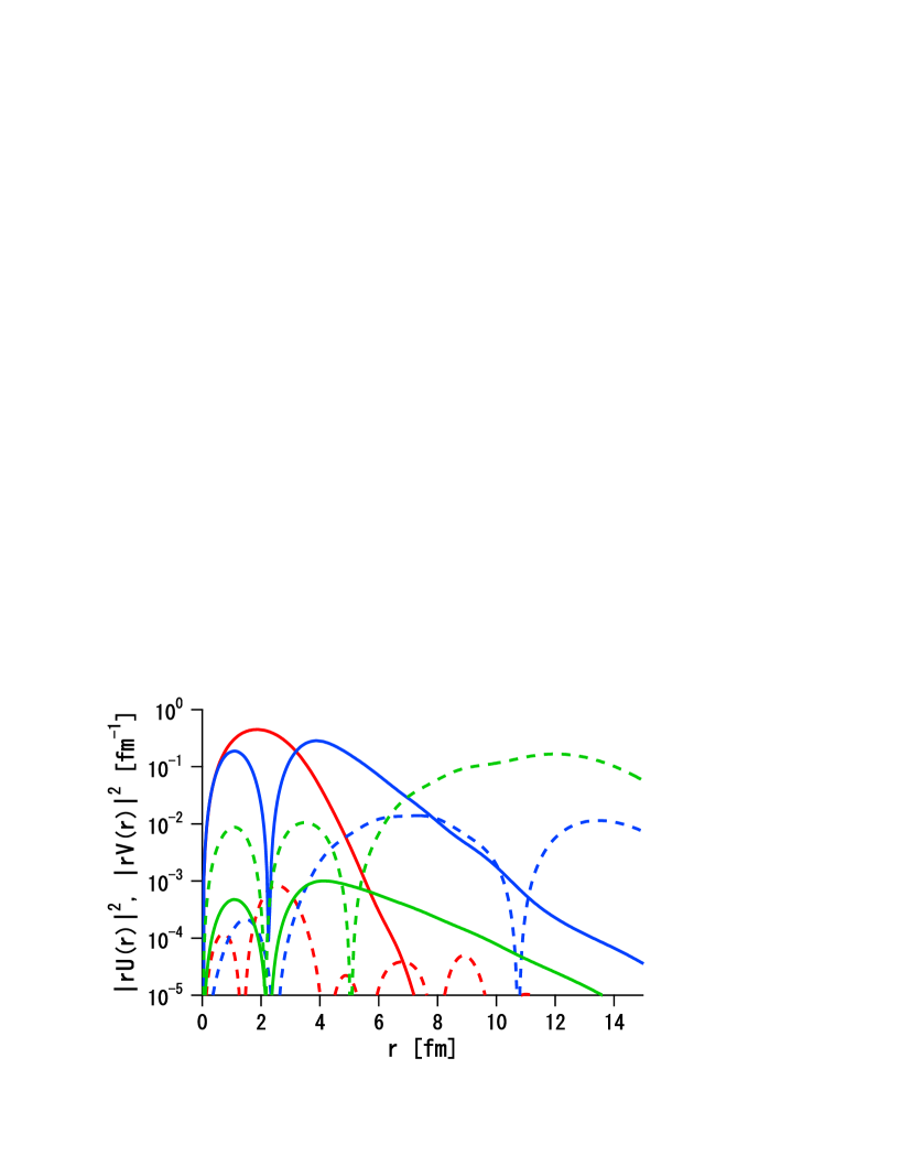
Figure 1: Wave functions of neutron $s_{1/2}$ q.p. levels in ²⁶O calculated with the D1S interaction. The colors distinguish the q.p. levels: The red, blue and green lines show the wave functions of the levels corresponding to the $0s_{1/2}$, $1s_{1/2}$ and $2s_{1/2}$ orbits, respectively. The full (dashed) curves represent $|r\,V^{(\ell j)}_{n}(r)|^{2}$ ($|r\,U^{(\ell j)}_{n}(r)|^{2}$) for each level.

We next look into the wave functions of the q.p. states, using Set C. Figure 1 shows the radial wave functions of the neutron q.p. levels in ²⁶O which correspond to the $0s_{1/2}$, $1s_{1/2}$ and $2s_{1/2}$ orbits, in terms of $|r\,V^{(\ell j)}_{n}(r)|^{2}$ and $|r\,U^{(\ell j)}_{n}(r)|^{2}$. In this calculation ²⁶O is so loosely bound with $\lambda\simeq-0.4\,\mathrm{MeV}$ that all q.p. levels would lie in the continuum, satisfying $\lambda+\epsilon_{n\ell j}>0$. In this regard the q.p. levels shown in Fig. 1 are considered to be resonance-like levels. For all the three q.p. states, whose q.p. energies distribute from $1.4\,\mathrm{MeV}$ to $40\,\mathrm{MeV}$, the energy-dependent exponential asymptotics in $r\,V^{(\ell j)}_{n}(r)$ are represented appropriately by the superposition of the GEM bases. We find oscillatory behavior in $r\,U^{(\ell j)}_{n}(r)$. In order to view how appropriately the oscillatory asymptotics are described, we define the following quantity from the Fourier transform of $r\,U^{(\ell j)}_{n}(r)$,

$$\Gamma_{n\ell j}(k)\equiv\frac{1}{\pi}\left|\int_{0}^{\infty}r\,U^{(\ell j)}_{n}(r)\,e^{ikr}\,dr\right|^{2}\,\left(=\Gamma_{n\ell j}(-k)\right)\,.$$ (19)

The scale of $\Gamma_{n\ell j}(k)$ is connected to the occupation probability of the q.p. level, via

$$\int_{0}^{\infty}\Gamma_{n\ell j}(k)\,dk=\int_{0}^{\infty}|U^{(\ell j)}_{n}(r)|^{2}\,r^{2}dr=1-\int_{0}^{\infty}|V^{(\ell j)}_{n}(r)|^{2}\,r^{2}dr\,.$$ (20)

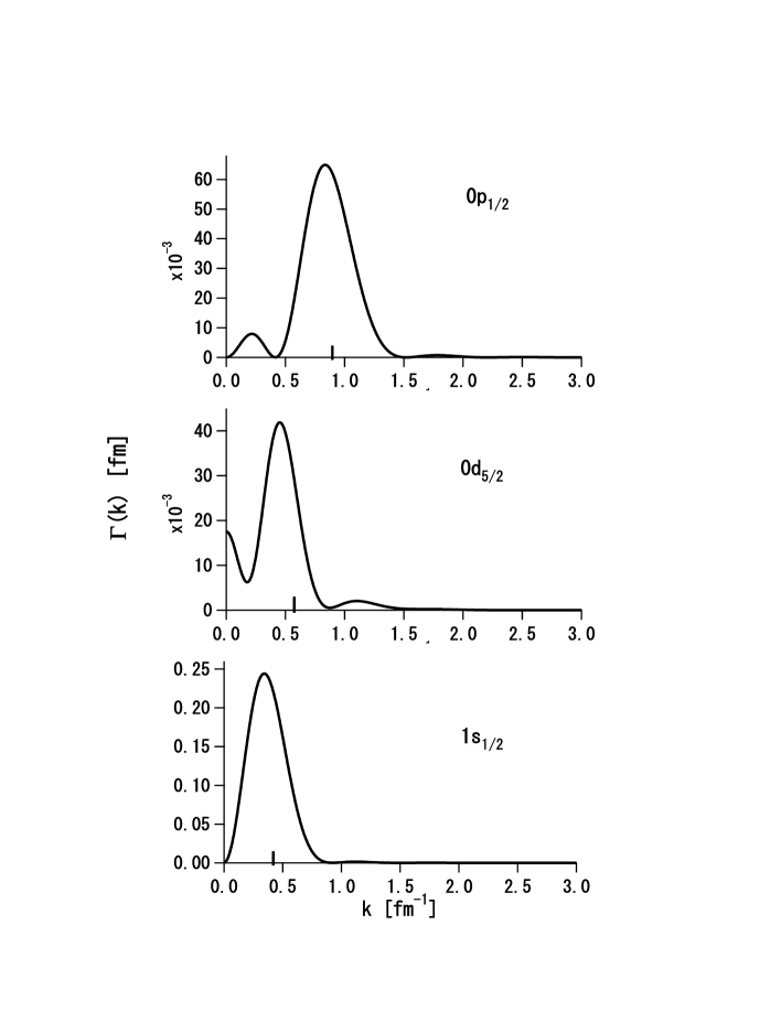
Figure 2: $\Gamma_{n\ell j}(k)$ of neutron q.p. levels in ²⁶O calculated with the D1S interaction. The values of $p^{(\ell j)}_{n}$ for individual q.p. levels are presented by the ticks on the horizontal axes.

If $U^{(\ell j)}_{n}(r)$ fulfills the asymptotics of Eq. (8) with $\lambda+\epsilon_{n\ell j}>0$, $\Gamma_{n\ell j}(k)$ should have a peak at $k=p^{(\ell j)}_{n}$. In Fig. 2 we show $\Gamma_{n\ell j}(k)$ for several low-lying q.p. levels of ²⁶O. Viewing the peaks of $\Gamma_{n\ell j}(k)$ at the positions compatible with the q.p. energies, we confirm that the energy-dependent oscillatory asymptotics are properly expressed through the superposition of the GEM bases.

In Table 2 we show the rms matter radii in HF and HFB obtained through the three basis-sets. Contribution of the center-of-mass motion is subtracted as in Ref. [4]. There is no significant difference among the bases up to ²⁴O, and this seems consistent with the results in Table 1. However, we find sizable basis-dependence in ^25,26O, although the energies do not differ significantly. In ²⁵O, where neutrons are not in the superfluid phase, the s.p. energy of $n0d_{3/2}$ in the HF scheme is vanishing ($\approx-0.05\,\mathrm{MeV}$). Thereby the calculated radius of ²⁵O is extremely sensitive to precise value of the s.p. energy. The ²⁶O case gives an illustration of the subtlety for the drip-line nuclei that have no discrete q.p. levels, as has been discussed in Sec. 3. In these cases in which the nuclei are very close to the neutron drip line, some physical quantities (e.g. nuclear radius) may depend on details of the calculation. Comparison of the radii between the HF and HFB calculations will be of a certain interest. The matter radii in the HFB scheme are similar to those in HF scheme around the $\beta$-stability line. However, in ²²O the HFB calculations give slightly larger radius than the HF calculations, primarily due to the partial occupation of $n1s_{1/2}$. Contrastingly, in ²⁶O the HFB radius is substantially smaller than the HF one in Sets B and C. This corresponds to the pairing anti-halo effect [12], although attention should be paid to the subtlety discussed in Sec. 3.

5.2 Dependence of shell structure on HF interaction

It has been argued that the spin-isospin nature of the $NN$ interaction could play a role in producing the new magic numbers [3]. We have developed an M3Y-type effective interaction called M3Y-P2 [4], which is applicable to the self-consistent HF calculations. Keeping the one-pion-exchange contribution to the central part of the $NN$ interaction, the M3Y-P2 interaction possesses reasonable spin-isospin nature, as was checked via the Landau-Migdal parameter in the nuclear matter. Within the self-consistent HF calculations, shell gaps at $N=16$ [4] and at $N=32$ [17] behave quite differently between M3Y-P2 and frequently used interactions such as D1S. With the D1S interaction the shell gap between $n1s_{1/2}$ and $n0d_{3/2}$ in the $N=16$ isotones is almost constant, as $Z$ changes from $8$ to $16$. On the contrary, the shell gap becomes narrower as $Z$ increases, if we adopt the M3Y-P2 interaction. Similar behavior has been found in the $N=32$ isotones. It should be pointed out that major difference lies around the $\beta$-stable region, rather than in the region close to the drip-line. We confirmed that the $Z$-dependence in the M3Y-P2 result is primarily ascribed to the contribution of the one-pion-exchange part.

The pair correlation can break the closed core, even in the spherical nuclei. This core breaking is realized in the HFB picture, unless the relevant shell gap is large enough. To investigate effects of the pair correlation in the region concerning the new magic numbers, we carry out the HFB calculations using the GEM algorithm for the $N=16$ and $32$ nuclei. While the D1S interaction has moderate pairing properties, the pairing character of the M3Y-P2 interaction is not realistic, since it has not been tuned. Here we always use the D1S interaction for the pairing interaction, i.e. to obtain the pair potential in the HFB equation (41), and examine dependence of the magic nature of $N=16$ and $32$ on the HF interactions, for which we take D1S and M3Y-P2. The $\ell\leq 4$ ($\ell\leq 5$) truncation is made for the $N=16$ ($N=32$) nuclei. For the basis-set, Set C in the preceding subsection is employed, with $K=12$.

In Table 3, the neutron pair energies in the $N=16$ and $32$ nuclei are compared between the two HF interactions. The pair energy is defined as contribution of the pairing tensor to the energy of the system. In the $N=16$ isotones, the D1S interaction does not give rise to the superfluidity for neutrons in $8\leq Z\leq 14$, as long as the spherical symmetry is assumed. In this regard, the D1S interaction provides a prediction that the $N=16$ magic number holds in the whole region of $8\leq Z\leq 14$. On the contrary, in the case that we use the M3Y-P2 interaction for the HF potential, the neutron pair energy increases as $Z$ goes from $8$ to $14$, i.e. from the drip-line region to the $\beta$-stable region. This behavior of the neutron pair energies, which is a reflection of shell structure in the HF scheme, is typically viewed in the difference between ²⁴O and ³⁰Si. Similar trend is seen in the $N=32$ isotones. While in ⁵²Ca the pair energy is not large and is close to each other between the two HF interactions, we find sizable interaction-dependence in ⁶⁰Ni, due to the difference in the shell structure in the HF regime.

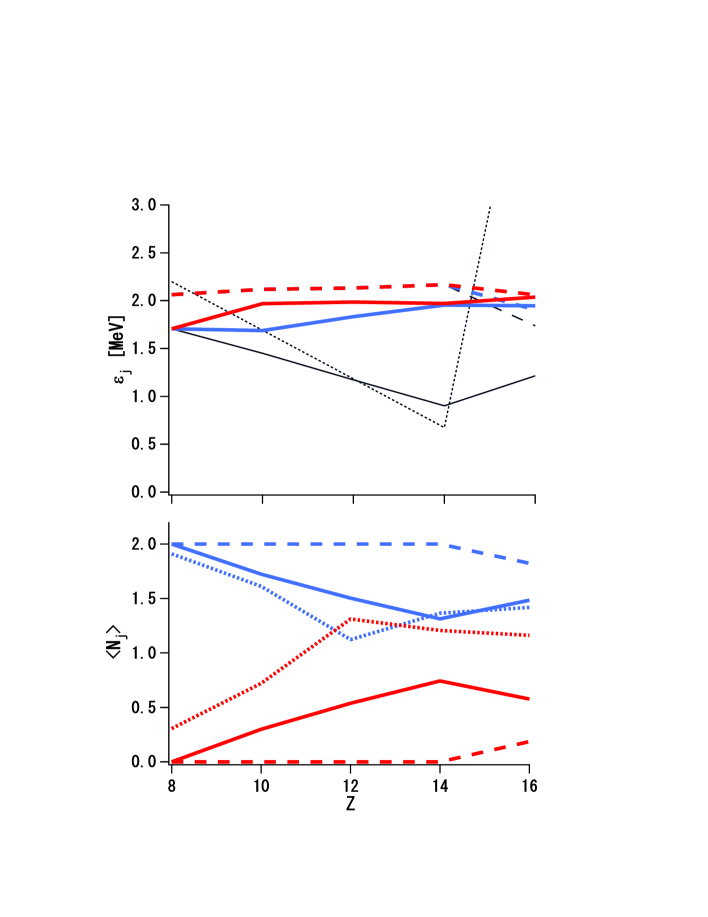
Figure 3: Neutron quasiparticle energies (upper panel) and neutron occupation numbers (lower panel) in the $Z=\mathrm{even}$, $N=16$ isotones. In both panels the red lines present the values of $0d_{3/2}$ in the HFB calculations, while the blue lines those of $1s_{1/2}$ if visible. The full (dashed) lines with each color are obtained with the M3Y-P2 (the D1S) HF interaction. The thin black lines indicate the HF results (see text for details). The black dotted line in the upper panel is obtained from the HF treatment of the USD Hamiltonian. The dotted lines with each color in the lower panel represent the occupation numbers obtained from the full shell-model calculation with the USD Hamiltonian.

Effects of the pair correlation on excitation spectra are basically viewed in the q.p. energies. In the upper panel of Fig. 3, the neutron q.p. energies corresponding to the $1s_{1/2}$ and $0d_{3/2}$ orbits are compared between the D1S and the M3Y-P2 interactions for the $Z=\mathrm{even}$, $N=16$ isotones. For reference, we also plot the s.p. energies measured from the Fermi energy in the HF approximation without the sign, as counterparts to the q.p. energies. We here define the Fermi energy as the arithmetic average of the HF energies of $n1s_{1/2}$ and $n0d_{3/2}$. Hence, half the shell gap between $n1s_{1/2}$ and $n0d_{3/2}$ is presented as the HF results. In the case that the neutron pair energy vanishes in the HFB calculations, we take the q.p. energies to be equal to their HF counterparts. We also show the values obtained from a HF picture within the $sd$-shell, employing the ‘USD’ shell-model Hamiltonian [18]. As pointed out in Ref. [3], the HF results indicate that the USD interaction yields significant $Z$-dependence of the shell gap, having qualitative similarity to the M3Y-P2 interaction. It should be noticed that the HF treatment of the shell-model Hamiltonian tends to give radical variation of the s.p. energies from nuclide to nuclide, in comparison with the self-consistent mean-field approaches, because effects of the rearrangement of the core are incorporated into the interaction within the valence shell in an effective manner.

The HF and the HFB energies coincide up to $Z=14$ in the calculations using the D1S interaction, because the nuclei are not in the superfluid phase. In the HFB results, the M3Y-P2 interaction provides almost constant q.p. energies of $n1s_{1/2}$ and $n0d_{3/2}$, which are close to those given by the D1S interaction. This is because the narrowing of the shell gap is compensated by the pairing gap to a considerable extent. It is suggested from the q.p. energies that the two interactions yield similar excitation spectra. In other words, the M3Y-P2 interaction does not seem to destroy the energy spectra predicted in the widely used interactions like D1S, despite the difference in physical contents. However, additional correlations could affect the energy levels considerably. It will be interesting to investigate influence of the correlations beyond HFB in these nuclei.

The occupation numbers of the relevant q.p. levels are depicted in the lower panel of Fig. 3. Due to the narrowing shell gap, we observe depletion of the $n1s_{1/2}$ occupation in the HFB results with M3Y-P2, as $Z$ grows from $8$ to $14$. This indicates, consistently with the behavior of the pair energies, that the magic nature of $N=16$ becomes weaker as $Z$ increases. Thus the spectroscopic factors of the neutron orbits could be useful in discriminating the two pictures; a picture based on the almost constant $N=16$ shell gap, and that on the decreasing shell gap for increasing $Z$ which may be compensated by the pairing gap. As shown in Fig. 3, the occupation numbers obtained with M3Y-P2 are compared to those in the full shell-model calculation using the USD Hamiltonian, except at $Z=12$ where influence of the quadrupole deformation seems important.

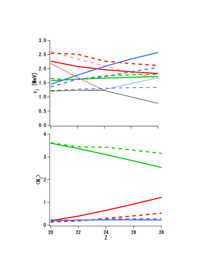
Figure 4: Neutron quasiparticle energies (upper panel) and neutron occupation numbers (lower panel) in the $Z=\mathrm{even}$, $N=32$ isotones. In both panels the red, blue and green lines present the values corresponding to the $0f_{5/2}$, $1p_{1/2}$ and $1p_{3/2}$ levels. The full (dashed) lines with each color are obtained with the M3Y-P2 (the D1S) HF interaction. The thick lines indicate the HFB results, while the thin lines the HF results. In the upper panel, the black color is used for the energy of the two levels adjacent to the Fermi energy in the HF results.

Figure 4 shows the q.p. energies and the occupation numbers of the levels corresponding to the $n1p_{3/2}$, $n0f_{5/2}$ and $n1p_{1/2}$ orbits, for the $Z=\mathrm{even}$, $N=32$ isotones. As the HF counterparts to the q.p. energies, we plot the s.p. energies measured from the Fermi energy, without the sign. The Fermi energy is taken to be the arithmetic average of the energies of the two levels nearest the $N=32$ gap (i.e. $1p_{3/2}$ and the lower level out of $0f_{5/2}$ and $1p_{1/2}$). As a result, the two levels have equal energy, which represent half the shell gap, in regard to the HF counterparts to the q.p. energies. These values are shown by the thin black lines in the upper panel of Fig. 4. As argued in Ref. [17], the D1S interaction gives almost constant shell gap in $20\leq Z\leq 28$, while M3Y-P2 yields erosion of the gap as $Z$ goes from $20$ to $28$. Furthermore, the s.p. energy difference between $n0f_{5/2}$ and $n1p_{3/2}$ changes more rapidly in the M3Y-P2 results than in the D1S ones. This gives rise to the inversion of $n0f_{5/2}$ and $n1p_{1/2}$ near $Z=24$ in the M3Y-P2 case, while such inversion does not occur in the D1S case. This shell structure in the HF scheme affects the HFB occupation numbers. Although the $N=32$ core does not close in the whole region of $20\leq Z\leq 28$ in the strict sense of the HFB theory, at $Z=20$ the occupation number of each orbit is not significantly different from the value assuming the $N=32$ closure, irrespectively of the HF potential. If we use the D1S interaction for the HF potential, this nature is almost preserved as $Z$ increases. In contrast, when we apply the M3Y-P2 interaction, leakage out of $n1p_{3/2}$ appreciably grows for increasing $Z$, mainly due to the pair excitation to $n0f_{5/2}$. Despite this difference in the physical picture, the q.p. energies are much less interaction-dependent, because the decreasing shell gap in M3Y-P2 is compensated by the increasing pairing gap to a certain extent. Therefore the excitation spectra will not differ much between the two HF interactions, unless disturbance due to the additional correlations is substantially strong. Yet the inversion of $n0f_{5/2}$ and $n1p_{1/2}$ occurs in the HFB results with M3Y-P2, which is not seen in the results with D1S.

6 Summary

Extending the previous work on the Hartree-Fock (HF) calculations based on the Gaussian expansion method (GEM), we develop a new method of implementing the Hartree-Fock-Bogolyubov (HFB) calculations. This method has two notable advantages: (i) It is efficient in describing the exponential and the oscillatory asymptotics of wave functions at large $r$, which depend on quasiparticle energy and could play a significant role in nuclei close to the drip lines. (ii) We can handle various effective interactions, including those inducing non-local nuclear currents.

The present method has been tested numerically in the oxygen isotopes with the Gogny D1S force, by assuming the spherical symmetry and the parity conservation. Three sets of GEM bases are tried and their results are compared; a set comprised of the real-range Gaussians, a set comprised of the complex-range Gaussians, and a set of their mixture. The last one gives the best results in the context of the variational principle. We have confirmed that both the exponential and the oscillatory asymptotics of the quasiparticle wave functions are properly described.

Relating to the new magic numbers in nuclei far from the $\beta$-stability, we have investigated interplay of the pair correlation and the shell gaps at $N=16$ and $32$. The Gogny D1S and the M3Y-P2 interactions are used for the HF interaction, while for the pair potential we always use the D1S interaction. Reflecting the interaction-dependence of the shell structure in the HF scheme, the M3Y-P2 case provides stronger $Z$-dependence of the superfluidity at $N=16$ and $32$ than the D1S case. While the q.p. energies do not differ significantly between the D1S and the M3Y-P2 interactions, suggesting that excitation spectra could resemble each other, the occupation numbers of neutron orbits reflect the interaction-dependence of the shell structure. The occupation numbers obtained from the M3Y-P2 interaction are comparable with those in the standard shell model, for the $N=16$ nuclei.

The author is grateful to Y. R. Shimizu for discussions. This work is financially supported in part as Grant-in-Aid for Scientific Research (B), No. 15340070, by the Ministry of Education, Culture, Sports, Science and Technology, Japan. Numerical calculations are performed on HITAC SR11000 at Institute of Media and Information Technology, Chiba University, and at Information Technology Center, University of Tokyo.

Appendices

Appendix A HFB equation for non-orthogonal bases

In this appendix we present the HFB theory in the case that non-orthogonal s.p. bases are adopted. We denote the creation (annihilation) operator associated with the s.p. basis $k$ by $c_{k}^{\dagger}$ ($c_{k}$). The non-orthogonality leads to the non-canonical commutation relations,

$$\{c_{k},c_{k^{\prime}}^{\dagger}\}=N_{kk^{\prime}}\,,\quad\{c_{k},c_{k^{\prime}}\}=\{c_{k}^{\dagger},c_{k^{\prime}}^{\dagger}\}=0\,,$$ (21)

where $\mathsf{N}=(N_{kk^{\prime}})$ is the norm matrix satisfying $N_{kk^{\prime}}^{\ast}=N_{k^{\prime}k}$ and being positive-definite. The generalized Bogolyubov transformation is defined by

$$\alpha_{i}^{\dagger}=\sum_{k}\left(U_{ki}\,c_{k}^{\dagger}+V_{ki}\,c_{k}\right)\,.$$ (22)

In the matrix representation, Eq. (22) can be expressed as

$$(\begin{array}[]{cc}\mathsf{\alpha}^{\dagger}&\mathsf{\alpha}\end{array})=(\begin{array}[]{cc}\mathsf{c}^{\dagger}&\mathsf{c}\end{array})\,\mathsf{W}\,;\quad\mathsf{W}=\left(\begin{array}[]{cc}\mathsf{U}&\mathsf{V}^{\ast}\\ \mathsf{V}&\mathsf{U}^{\ast}\end{array}\right)\,.$$ (23)

Obtained as a solution of the HFB equation, $\alpha_{i}^{\dagger}$ and $\alpha_{i}$ obey the canonical commutation relations,

$$\{\alpha_{i},\alpha_{i^{\prime}}^{\dagger}\}=\delta_{ii^{\prime}}\,,\quad\{\alpha_{i},\alpha_{i^{\prime}}\}=\{\alpha_{i}^{\dagger},\alpha_{i^{\prime}}^{\dagger}\}=0\,.$$ (24)

This indicates

$$\overline{\mathsf{W}}\,\mathsf{N}^{\prime}\,\mathsf{W}=1\,,\quad\mathsf{W}\,\overline{\mathsf{W}}=\mathsf{N}^{\prime-1}\,;\quad\mathsf{N}^{\prime}=\left(\begin{array}[]{cc}\mathsf{N}&0\\ 0&\mathsf{N}^{\ast}\end{array}\right)\,,$$ (25)

i.e.,

$$\overline{\mathsf{U}}\,\mathsf{N}\,\mathsf{U}+\overline{\mathsf{V}}\,\mathsf{N}^{\ast}\,\mathsf{V}=1\,, \mathsf{V}^{\mathrm{T}}\,\mathsf{N}\,\mathsf{U}+\mathsf{U}^{\mathrm{T}}\,\mathsf{N}^{\ast}\,\mathsf{V}=0\,,$$

$$\mathsf{U}\,\overline{\mathsf{U}}+\mathsf{V}^{\ast}\,\mathsf{V}^{\mathrm{T}}=\mathsf{N}^{-1}\,, \mathsf{U}\,\overline{\mathsf{V}}+\mathsf{V}^{\ast}\,\mathsf{U}^{\mathrm{T}}=0\,.$$ (26)

We here use the expression $\overline{\mathsf{A}}=(\mathsf{A}^{\ast})^{\mathrm{T}}$, instead of $\mathsf{A}^{\dagger}$, to avoid confusion with the hermitian conjugation of operators. The inversion of the Bogolyubov transformation of Eq. (23) yields

$$(\begin{array}[]{cc}\mathsf{c}^{\dagger}&\mathsf{c}\end{array})=(\begin{array}[]{cc}\mathsf{\alpha}^{\dagger}&\mathsf{\alpha}\end{array})\,\overline{\mathsf{W}}\,\mathsf{N}^{\prime}\,.$$ (27)

We define the density matrix and the pairing tensor by

$$(\mathsf{N}\,\mathsf{\rho}\,\mathsf{N})_{kk^{\prime}}~{}=~{}\langle\Phi|c_{k^{\prime}}^{\dagger}c_{k}|\Phi\rangle = (\mathsf{N}\,\mathsf{V}^{\ast}\,\mathsf{V}^{\mathrm{T}}\,\mathsf{N})_{kk^{\prime}}\,,$$

$$(\mathsf{N}\,\mathsf{\kappa}\,\mathsf{N}^{\ast})_{kk^{\prime}}~{}=~{}\langle\Phi|c_{k^{\prime}}c_{k}|\Phi\rangle = \langle\Phi|c_{k}^{\dagger}c_{k^{\prime}}^{\dagger}|\Phi\rangle^{\ast}~{}=~{}(\mathsf{N}\,\mathsf{V}^{\ast}\,\mathsf{U}^{\mathrm{T}}\,\mathsf{N}^{\ast})_{kk^{\prime}}\,,$$ (28)

where $|\Phi\rangle$ is the HFB vacuum. This HFB vacuum $|\Phi\rangle$ satisfies $\alpha_{n\ell jm}|\Phi\rangle=0$ and $\langle\Phi|\Phi\rangle=1$. Equation (28) obviously indicates

$$\rho_{kk^{\prime}}=(\mathsf{V}^{\ast}\,\mathsf{V}^{\mathrm{T}})_{kk^{\prime}}\,,\quad\kappa_{kk^{\prime}}=(\mathsf{V}^{\ast}\,\mathsf{U}^{\mathrm{T}})_{kk^{\prime}}\,.$$ (29)

In the HFB approximation the expectation value of the number operator is adjusted to the actual particle number $n$. This constraint is expressed by $\mathrm{Tr}(\mathsf{N}\,\mathsf{\rho})=n$. The HF Hamiltonian and the pair potential are defined by

$$h_{kk^{\prime}}~{}=~{}\frac{\delta}{\delta\rho_{kk^{\prime}}}\langle\Phi|\hat{H}|\Phi\rangle = \langle\Phi|\{[c_{k},\hat{H}],c_{k^{\prime}}^{\dagger}\}|\Phi\rangle\,,$$

$$\Delta_{kk^{\prime}}~{}=~{}\frac{\delta}{\delta\kappa_{kk^{\prime}}^{\ast}}\langle\Phi|\hat{H}|\Phi\rangle = \langle\Phi|\{[c_{k},\hat{H}],c_{k^{\prime}}\}|\Phi\rangle\,,$$ (30)

from which the following HFB Hamiltonian matrix is obtained,

$$\mathsf{\mathcal{H}}=\left(\begin{array}[]{cc}\mathsf{h}-\lambda&\mathsf{\Delta}\\ -\mathsf{\Delta}^{\ast}&-\mathsf{h}^{\ast}+\lambda\end{array}\right)\,,$$ (31)

with the chemical potential $\lambda$. The HFB equation for the non-orthogonal bases has the following form of the generalized eigenvalue equation,

$$\mathsf{\mathcal{H}}\,\mathsf{W}=\mathsf{N}^{\prime}\,\mathsf{W}\left(\begin{array}[]{cc}\mathsf{\epsilon}&0\\ 0&-\mathsf{\epsilon}\end{array}\right)\,;\quad\mathsf{\epsilon}=\mathrm{diag}(\epsilon_{i})\,.$$ (32)

It is commented that, because $\mathsf{N}$ is a Hermite positive-definite matrix, it can be decomposed as $\mathsf{N}=\mathsf{L}\,\overline{\mathsf{L}}$ by using a lower-triangular matrix $\mathsf{L}$. Multiplication of $\mathsf{c}$ by $\mathsf{L}^{-1}$ gives an orthogonalization of the s.p. bases, and the canonical commutation relation follows;

$$\{(\mathsf{L}^{-1}\,\mathsf{c})_{k},((\mathsf{L}^{-1})^{\ast}\,\mathsf{c}^{\dagger})_{k^{\prime}}\}=\delta_{kk^{\prime}}\,.$$ (33)

All the equations return to those in the usual HFB theory for the orthogonal bases, by multiplying by $\mathsf{L}^{-1}$ appropriately.

For the Hamiltonian consisting of the one-body term $\hat{K}$ and the two-body interaction $\hat{V}$, we obtain

$$\langle\Phi|\hat{H}|\Phi\rangle=\sum_{k_{1}k_{2}}\langle k_{2}|\hat{K}|k_{1}\rangle\,\rho_{k_{1}k_{2}}+\frac{1}{4}\sum_{k_{1}k_{2}k_{3}k_{4}}\langle k_{3}k_{4}|\hat{V}|k_{1}k_{2}\rangle\,(2\rho_{k_{1}k_{3}}\rho_{k_{2}k_{4}}+\kappa_{k_{1}k_{2}}\kappa^{\ast}_{k_{3}k_{4}})\,,$$ (34)

where $|k\rangle=c_{k}^{\dagger}|0\rangle$ and $|kk^{\prime}\rangle=c_{k}^{\dagger}c_{k^{\prime}}^{\dagger}|0\rangle$, with $|0\rangle$ representing the particle vacuum satisfying $c_{k}|0\rangle=0$. Equation (34) derives

$$h_{kk^{\prime}} = \langle k^{\prime}|\hat{K}|k\rangle+\sum_{k_{1}k_{2}}\langle k^{\prime}k_{2}|\hat{V}|kk_{1}\rangle\,\rho_{k_{1}k_{2}}\,,$$

$$\Delta_{kk^{\prime}} = \frac{1}{2}\sum_{k_{1}k_{2}}\langle kk^{\prime}|\hat{V}|k_{1}k_{2}\rangle\,\kappa_{k_{1}k_{2}}\,.$$ (35)

For interactions having the form of Eq. (15), rearrangement terms for $v_{12}^{(\mathrm{DD})}$, which emerge via variation of $\rho^{\alpha}$, should be taken into account.

Appendix B HFB equation with spherical symmetry

By adopting the spherically symmetric s.p. bases $k=(\nu\ell jm)$ and $k^{\prime}=(\nu^{\prime}\ell^{\prime}j^{\prime}m^{\prime})$, the norm matrix $\mathsf{N}$ is simplified as in Eq. (3),

$$N_{kk^{\prime}}=\delta_{\ell\ell^{\prime}}\delta_{jj^{\prime}}\delta_{mm^{\prime}}\cdot N^{(\ell j)}_{\nu\nu^{\prime}}\,.$$ (36)

If we assume the spherical symmetry on the HFB fields, the q.p. state is taken to be $i=(n\ell jm)$, and the $U$- and $V$-coefficients in Eq. (22) have the form

$$U_{k^{\prime}i}=\delta_{\ell\ell^{\prime}}\delta_{jj^{\prime}}\delta_{mm^{\prime}}\cdot U^{(\ell j)}_{\nu^{\prime}n}\,,\quad V_{k^{\prime}i}=\delta_{\ell\ell^{\prime}}\delta_{jj^{\prime}}\delta_{m-m^{\prime}}(-)^{j+m}\cdot V^{(\ell j)}_{\nu^{\prime}n}\,.$$ (37)

Equation (26) is then reduced to

$$\overline{\mathsf{U}^{(\ell j)}}\,\mathsf{N}^{(\ell j)}\,\mathsf{U}^{(\ell j)}+\overline{\mathsf{V}^{(\ell j)}}\,\mathsf{N}^{(\ell j)\ast}\,\mathsf{V}^{(\ell j)}=1\,, \mathsf{V}^{(\ell j)\mathrm{T}}\,\mathsf{N}^{(\ell j)}\,\mathsf{U}^{(\ell j)}-\mathsf{U}^{(\ell j)\mathrm{T}}\,\mathsf{N}^{(\ell j)\ast}\,\mathsf{V}^{(\ell j)}=0\,,$$

$$\mathsf{U}^{(\ell j)}\,\overline{\mathsf{U}^{(\ell j)}}+\mathsf{V}^{(\ell j)\ast}\,\mathsf{V}^{(\ell j)\mathrm{T}}=\mathsf{N}^{(\ell j)-1}\,, \mathsf{U}^{(\ell j)}\,\overline{\mathsf{V}^{(\ell j)}}-\mathsf{V}^{(\ell j)\ast}\,\mathsf{U}^{(\ell j)\mathrm{T}}=0\,.$$ (38)

Analogously to Eq. (37), the density matrix, the pairing tensor, the HF Hamiltonian and the pair potential are taken as

$$\rho_{kk^{\prime}}=\delta_{\ell\ell^{\prime}}\delta_{jj^{\prime}}\delta_{mm^{\prime}}\cdot\rho^{(\ell j)}_{\nu\nu^{\prime}}\,; \rho^{(\ell j)}_{\nu\nu^{\prime}}=(\mathsf{V}^{(\ell j)\ast}\,\mathsf{V}^{(\ell j)\mathrm{T}})_{\nu\nu^{\prime}}\,,$$

$$\kappa_{kk^{\prime}}=\delta_{\ell\ell^{\prime}}\delta_{jj^{\prime}}\delta_{m-m^{\prime}}(-)^{j-m}\cdot\kappa^{(\ell j)}_{\nu\nu^{\prime}}\,; \kappa^{(\ell j)}_{\nu\nu^{\prime}}=(\mathsf{V}^{(\ell j)\ast}\,\mathsf{U}^{(\ell j)\mathrm{T}})_{\nu\nu^{\prime}}\,,$$ (39)

and

$$h_{kk^{\prime}}=\delta_{\ell\ell^{\prime}}\delta_{jj^{\prime}}\delta_{mm^{\prime}}\cdot h^{(\ell j)}_{\nu\nu^{\prime}}\,,\quad\Delta_{kk^{\prime}}=\delta_{\ell\ell^{\prime}}\delta_{jj^{\prime}}\delta_{m-m^{\prime}}(-)^{j-m}\cdot\Delta^{(\ell j)}_{\nu\nu^{\prime}}\,.$$ (40)

Note that $\kappa^{(\ell j)}_{\nu\nu^{\prime}}=\kappa^{(\ell j)}_{\nu^{\prime}\nu}$ and $\Delta^{(\ell j)}_{\nu\nu^{\prime}}=\Delta^{(\ell j)}_{\nu^{\prime}\nu}$. With these replacements the HFB equation under the spherical symmetry is written as

$$\mathsf{\mathcal{H}}^{(\ell j)}\,\mathsf{W}^{(\ell j)}=\mathsf{N}^{\prime(\ell j)}\,\mathsf{W}^{(\ell j)}\left(\begin{array}[]{cc}\mathsf{\epsilon}^{(\ell j)}&0\\ 0&-\mathsf{\epsilon}^{(\ell j)}\end{array}\right)\,;\quad\mathsf{\epsilon}^{(\ell j)}=\mathrm{diag}(\epsilon_{n\ell j})\,,$$ (41)

where

$$\mathsf{\mathcal{H}}^{(\ell j)}=\left(\begin{array}[]{cc}\mathsf{h}^{(\ell j)}-\lambda&\mathsf{\Delta}^{(\ell j)}\\ \mathsf{\Delta}^{(\ell j)\ast}&-\mathsf{h}^{(\ell j)\ast}+\lambda\end{array}\right)\,,\quad\mathsf{W}^{(\ell j)}=\left(\begin{array}[]{cc}\mathsf{U}^{(\ell j)}&\mathsf{V}^{(\ell j)\ast}\\ -\mathsf{V}^{(\ell j)}&\mathsf{U}^{(\ell j)\ast}\end{array}\right)\,,$$ (46)

$$\mathsf{N}^{\prime(\ell j)}=\left(\begin{array}[]{cc}\mathsf{N}^{(\ell j)}&0\\ 0&\mathsf{N}^{(\ell j)\ast}\end{array}\right)\,.$$ (49)

Table 1: HF and HFB energies (MeV) of ^14-26O, calculated with the D1S interaction.

nuclide	HF				HFB
	Set A	Set B	Set C		Set A	Set B	Set C
14O	$-~{}99.522$	$-~{}99.533$	$-~{}99.559$		—	$-~{}99.586$	$-~{}99.613$
15O	$-114.467$	$-114.479$	$-114.509$		$-114.467$	$-114.479$	$-114.509$
16O	$-129.477$	$-129.483$	$-129.515$		$-129.477$	$-129.483$	$-129.515$
17O	$-134.518$	$-134.521$	$-134.548$		$-134.518$	$-134.521$	$-134.548$
18O	$-139.711$	$-139.710$	$-139.734$		$-142.283$	$-142.286$	$-142.309$
19O	$-145.079$	$-145.076$	$-145.096$		$-146.391$	$-146.391$	$-146.411$
20O	$-150.644$	$-150.639$	$-150.657$		$-153.329$	$-153.331$	$-153.350$
21O	$-156.425$	$-156.419$	$-156.434$		$-156.425$	$-156.419$	$-156.434$
22O	$-162.438$	$-162.432$	$-162.444$		$-162.540$	$-162.546$	$-162.563$
23O	$-165.278$	$-165.298$	$-165.321$		$-165.278$	$-165.298$	$-165.321$
24O	$-168.540$	$-168.568$	$-168.595$		$-168.540$	$-168.568$	$-168.595$
25O	$-168.082$	$-168.084$	$-168.134$		$-168.082$	$-168.084$	$-168.134$
26O	$-167.942$	$-167.935$	$-167.995$		$-169.248$	$-169.266$	$-169.304$

Table 2: Rms radii (fm) of ^14-26O in the HF and HFB calculations with the D1S interaction.

nuclide	HF				HFB
	Set A	Set B	Set C		Set A	Set B	Set C
14O	$2.532$	$2.530$	$2.530$		—	$2.535$	$2.534$
15O	$2.570$	$2.568$	$2.568$		$2.570$	$2.568$	$2.568$
16O	$2.609$	$2.607$	$2.606$		$2.609$	$2.607$	$2.606$
17O	$2.663$	$2.662$	$2.661$		$2.663$	$2.662$	$2.661$
18O	$2.712$	$2.711$	$2.711$		$2.707$	$2.706$	$2.705$
19O	$2.756$	$2.755$	$2.755$		$2.755$	$2.754$	$2.753$
20O	$2.796$	$2.795$	$2.795$		$2.794$	$2.793$	$2.793$
21O	$2.832$	$2.831$	$2.831$		$2.832$	$2.831$	$2.831$
22O	$2.864$	$2.863$	$2.863$		$2.875$	$2.874$	$2.874$
23O	$2.950$	$2.947$	$2.948$		$2.950$	$2.947$	$2.948$
24O	$3.016$	$3.013$	$3.014$		$3.016$	$3.013$	$3.014$
25O	$3.133$	$3.102$	$3.119$		$3.133$	$3.102$	$3.119$
26O	$3.205$	$3.177$	$3.197$		$3.203$	$3.159$	$3.164$

Table 3: Interaction-dependence of neutron pair energies (MeV) in $N=16$ and $32$ nuclei.

nuclide	D1S	M3Y-P2
24O	$0.000$	$0.000$
30Si	$0.000$	$-3.911$
52Ca	$-2.122$	$-2.224$
60Ni	$-4.825$	$-7.055$

References

- [1] I. Tanihata, Prog. Part. Nucl. Phys. 35 (1995) 505.
- [2] A. Ozawa, T. Kobayashi, T. Suzuki, K. Yoshida and I. Tanihata, Phys. Rev. Lett. 84 (2000) 5493 R. Kanungo, I. Tanihata and A. Ozawa, Phys. Lett. B 528 (2002) 58.
- [3] T. Otsuka et al., Phys. Rev. Lett. 87 (2001) 082502.
- [4] H. Nakada, Phys. Rev. C 68 (2003) 014316.
- [5] A. L. Goodman, Advances in Nuclear Physics vol. 11, edited by J. W. Negele and E. Vogt (Plenum, New York, 1979), p. 263.
- [6] H. Nakada and M. Sato, Nucl. Phys. A 699 (2002) 511; ibid. 714 (2003) 696.
- [7] M. V. Stoitsov, J. Dobaczewski, P. Ring and S. Pittel, Phys. Rev. C 61 (2000) 034311.
- [8] M. Kamimura, Phys. Rev. A 38 (1988) 621.
- [9] E. Hiyama, Y. Kino and M. Kamimura, Prog. Part. Nucl. Phys. 51 (2003) 223.
- [10] H. Kameyama, M. Kamimura and Y. Fukushima, Phys. Rev. C 40 (1989) 974.
- [11] J. Dobaczewski, H. Flocard and J. Treiner, Nucl. Phys. A 422 (1984) 103.
- [12] K. Bennaceur, J. Dobaczewski and M. Płoszajczak, Phys. Lett. B 496 (2000) 154.
- [13] J. Dechargé and D. Gogny, Phys. Rev. C 21 (1980) 1568.
- [14] J. F. Berger, M. Girod and D. Gogny, Comp. Phys. Comm. 63 (1991) 365.
- [15] D. Guillemaud-Mueller et al., Phys. Rev. C 41 (1990) 937; M. Fauerbach et al., Phys. Rev. C 53 (1996) 647.
- [16] Y. R. Shimizu, private communication.
- [17] H. Nakada, Proceedings of the International Symposium “A New Era of Nuclear Structure Physics, edited by Y. Suzuki, M. Matsuo, S. Ohya and T. Ohtsubo, p. 184 (World Scientific, Singapore, 2004).
- [18] B. A. Brown, W. A. Richter, R. E. Julies and B. H. Wildenthal, Ann. Phys. (N.Y.) 182 (1988) 191.