On a variational principle model for the Nuclear Caloric curve

Abstract

Following the lead of a recent work we perform a variational principle model calculation for the nuclear caloric curve. A Skyrme type interaction with and without momentum dependence is used. The calculation is done for a large nucleus, i.e, in the nuclear matter limit. Thus we address the issue of volume fragmentation only. Nonetheless the results are similar to the previous, largely phenomenological calculation for a finite nucleus. We find the onset of fragmentation can be sudden as a function of temperature/excitation energy.

I Introduction

At low excitation energy the nucleus deexcites by binary sequential decay. This is envisaged by the compound nucleus hypothesis. It is usually believed that beyond a certain excitation, binary decay gives way to simultaneous break up [1]. This break up may well depend upon the details of collision, i.e., whether the energy was pumped in by heavy ion collisions or say, by a proton hitting a nucleus. For multifragmentation, it is conjectured that the nucleus expands to three/four times the normal volume and breaks up into various fragments, dictated by phase space. Calculations based on this picture have been successful in fitting many data. The SMM (statistical multifragmentation model) uses these ideas and predicted (well before any experiments) that one should see a maximum in the specific heat at temperatures around 5 MeV [2]. This was indeed found [3]. The appearence of a maximum in the specific heat led to a very interesting speculation that this may be a signature of phase transition. This is more dramatically demonstrated in the canoncal thermodynamic model (which is in the same spirit as the SMM but is much easier to implement). Here at low temperature there is a large blob of matter which breaks up into many pieces and the maximum in specific heat is obtained in this region. The thermodynamic model can be extrapolated to large numbers of particles. In this limit it is shown that the break up is very sudden as a function of temperature. This is a case of first order phase transition and the maximum of specific heat is obtained at the phase transition [4].

The beginning of such models started with Bevalac energy collisions where it was natural to assume that the system formed by collisions is first compressed and then begins to decompress. During the decompression stage, the products in terms of mass numbers, velocities etc. will evolve finally reaching a just streaming stage. While the changes will be continuous one can probably get an adequate description by assuming that all the changes can be described by assuming a constant freeze-out volume and doing a phase-space calculation (thermodynamics) at this volume. One can use the Boltzmann-Uehling-Uhlenbeck microscopic simulations [5] in support of an initial compression, followed by expansion and finally free streaming.

It is of course clear that a calculation of the caloric curve based on such models is not, in any simple way, connected to a variational principle. The present work is inspired by a recent calculation which showed that, in a different model based on a variational principle, a plateau in the caloric curve (hence a maximum in specific heat) can be reached in mononuclear configurations as well [6]. In this model, the nucleus expands when excitation energy is pumped in. Adopt a reasonable density profile for the ground state and assume that when energy is pumped into the nucleus, it expands in a self-similar fashion, i.e., $\rho(r,c)=c^{3}\rho(rc)$ where $c$ is a function of the excitation energy $e^{*}$. This excitation energy $e^{*}$ consists of two parts: a thermal part and a compression part which, as a function of density, increases quadratically about the ground state density [7]. At a given excitation energy, the nucleus expands till it reaches the maximum entropy (this is the variational principle of the calculation). Effects of interaction on entropy is taken through a parametrisation of $m^{*}/m$ where $m^{*}$ is the effective mass. A temperature is defined microcanonically. The authors then find that when they plot temperature against excitation energy, a plateau is found around 5 to 6 MeV.

Our investigation addresses the question of mononuclear configuration but with the following restriction . There is no surface in our calculation thus we are investigating break up as a volume effect. Stated differently, our calculation refers to nuclear matter. This restriction was dictated by our desire to do a more microscopic calculation. In [6] excitation energy is fixed. We do calculations first with fixed temperatures (this is a more well-known practice in nuclear physics) but then also do calculations with fixed energies. In both the approaches, the nucleus first expands as the temperature increases, a plateau is reached but then the nucleus breaks up quite suddenly. Once the nucleus breaks up, the model gives no guidance how the caloric curve is to be calculated further, into higher energy. In order to continue one needs to formulate a different model.

II Temparure dependent mean field theory

A familiar model in nuclear physics which allows study of the caloric curve in mononuclear configurations is the temparature dependent mean field model (Hartee-Fock and/or Thomas-Fermi model). This has certain advantages. When one does a standard mean field calculation at a fixed temparture, one minimises the free energy $F=E-TS$ [8]. This means that when we get the self-consistent solution at a given temperature, we have obtained a solution which has zero pressure. If we draw a caloric curve with energies of these solutions this caloric curve pertains to zero pressure. The specific heat that we will get will be $c_{p}$ with $p=0$.

Investigation of the caloric curve with temperature-dependent Thomas-Fermi theory was done in the past [9]. For nuclei ¹⁵⁰Sm and ⁸⁵Kr caloric curves were drawn and a maximum in specific heat at temperature $\approx$10 MeV was found. But there is ambiguity whether the systems stay mononuclear or not. The cause of the ambiguity is this. In finite temperature mean field theory (whether Thomas-Fermi or Hartree-Fock) single particle states in the continuum are admixed through the finite temperature occupation factors. These calculations are done in a finite box and because of this admixture to the continuum, the resulting density distributions become strongly dependent on the volume of the box. Thus in Fig. 2. of [9] at temperature 10 MeV if the calculation for ¹⁵⁰Sm is done by enclosing in a volume which is 4 times the normal nuclear volume one still has a compact system with a central density and a surface. One would be tempted to call this a mononuclear system. The density profile is totally different if the same calculation is done where the confining volume is 8 times the normal volume. Now the density is smeared out almost uniformly in the confining volume which would be the characteristics of a non-interacting gas. Although the densities alter a great deal, the maximum in the specific heat does not change much (close to 10 MeV in both the cases) but the widths of the specific heat do.

III Volume break up in finite temperature mean field theory

We can study the volume break up by working in the nuclear matter limit. This is pursued in this work. For a fixed temperature we do calculations for different densities. The density where the free energy per particle is minimised is the solution for this temperature; $e^{*}$ of this solution is the appropriate $e^{*}$ for this temperature. As expected, starting from zero temperature, the system expands. The minima of free energy drop to lower and lower density as the temperature increases. But beyond a certain temperature, the minimum in free energy disappears. The nucleus will now break apart. This happens just after $T$ flattens out as a function of $e^{*}$. This is shown in figs. 1 and 2.

We give some details of the calculation. We use the mometum dependent mean field of [10, 11]. The potential energy density is given by

$$v(\rho)=\frac{A}{2}\frac{\rho^{2}}{\rho_{0}}+\frac{B}{\sigma+1}\frac{\rho^{\sigma+1}}{\rho_{0}^{\sigma}}+\frac{C}{\rho_{0}}\int\int d^{3}pd^{3}p^{\prime}\frac{f(\vec{r},\vec{p})f(\vec{r},\vec{p}^{\prime})}{1+[\frac{\vec{p}-\vec{p}^{\prime}}{\Lambda}]^{2}}$$ (1)

Here $f(\vec{r},\vec{p})$ is phase-space density. In nuclear matter, at zero temperature $f(\vec{r},\vec{p})=\frac{4}{h^{3}}\Theta(p_{F}-p)$ where 4 takes care of spin-isospin degeneracy. At finite temperature the theta function $\Theta(p_{F}-p)$ is replaced by Fermi occupation factor (see details below). The potential felt by a particle is

$$u(\rho,\vec{p})=A[\frac{\rho}{\rho_{0}}]+B[\frac{\rho}{\rho_{0}}]^{\sigma}+2\frac{C}{\rho_{0}}\int d^{3}p^{\prime}\frac{f(\vec{r},\vec{p}^{\prime})}{1+[\frac{\vec{p}-\vec{p}^{\prime}}{\Lambda}]^{2}}$$ (2)

Here $A=$-110.44 Mev, $B$=140.9 MeV, $C$=-64.95 MeV, $\rho_{0}=0.16fm^{-3}$, $\sigma$=1.24 and $\Lambda=1.58p_{F}^{0}$. This gives in nuclear matter binding energy per particle=16 MeV, saturation density $\rho_{0}=.16fm^{-3}$, compressibility $K$=215 MeV and $m^{*}/m$=.67 at the fermi energy; $u(\rho,p)$ gives the correct general behaviour of the real part of the optical potential as a function of incident energy. A comparison of $u(\rho,p)$ with that derived from UV14+UVII potential in cold nuclear matter can be found in [11]. The specific functional form of the momentum dependent part arises from the Fock term of an Yukawa potential. Mean fields given by eqs. (1) and (2) have been widely tested for flow data [12] and give very good agreement.

To do a finite temperature calculation the following steps have to be executed. We need to find the occupation probability

$$n[\epsilon(p)]=\frac{1}{e^{\beta[\epsilon(p)-\mu]}+1}$$ (3)

for a given temperature $1/\beta$ and density $\rho$. If $\epsilon(p)$ were known a priori, this would merely entail finding the chemical potential from

$$\rho=\frac{16\pi}{h^{3}}\int_{0}^{\infty}p^{2}n[\epsilon(p)]dp$$ (4)

But the expression for $\epsilon(p)$ is

$$\epsilon(p)=\frac{p^{2}}{2m}+A[\frac{\rho}{\rho_{0}}]+B[\frac{\rho}{\rho_{0}}]^{\sigma}+R(\rho,p)$$ (5)

where at finite temperature

$$R(\rho,p)=2\frac{C}{\rho_{0}}\frac{4}{h^{3}}\int d^{3}p^{\prime}n[\epsilon(p^{\prime})]\times\frac{1}{1+[\frac{\vec{p}-\vec{p}^{\prime}}{\Lambda}]^{2}}$$ (6)

Thus knowing $R(\rho,p)$ requires knowing $n[\epsilon(p^{\prime})]$ already for all values of $p^{\prime}$. This self-consistency condition can be fulfilled by an iterative procedure (details can be found in [11]).

To calculate pressure, we use the thermodynamic identity $pV=-E+TS+\mu N$ which then gives

$$p=a+b+c$$ (7)

Here

$$a=-v-\frac{16\pi}{h^{3}}\int_{0}^{\infty}dp\frac{p^{4}}{2m}n[\epsilon(p)]$$ (8)

where $v$ is given by eq. (1) and the second term is the contribution from the kinetic energy.

$$b=-T\frac{16\pi}{h^{3}}\int_{0}^{\infty}p^{2}[n\ln n+(1-n)\ln(1-n)]dp$$ (9)

The term $c$ is $\mu\rho$. The free energy per particle is $-(a+b)/\rho$. The test $p=0$ when the minimum of free energy is reached provides a sensible test of numerical accuracy.

Fig.1 shows a plot of free energy per particle against temperature. There is no minimum in free energy at 12 MeV although at lower temperatures shown in the figure, minima are seen. The figure therefore suggests that as the system approaches the temperature of 12 MeV, it will break up. In Fig.2 we show the caloric curve. The temperature flattens against $e^{*}$, momentarily reaches zero slope (more about the slope in a later section) and we reach the end of the model. At higher temperatures there is no minimum in free energy and so to continue a new principle has to be postulated. If now we use a freeze-out volume then we have reached the more widely used approach for the caloric curve.

We have compared the caloric curve with the one computed with the low enrgy expansion of the Fermi-gas model: $e^{*}=aT^{2}$. As in [6], with momentum dependence, the caloric curve is initially above the Fermi-gas model curve and meets the Fermi-gas curve at a later point. The details of the caloric curve depends upon $m^{*}/m$. Normally one writes $m^{*}/m=m_{k}m_{\omega}$. Sobotka et al. adopt a phenomenolgical expression for $m_{k}$ and $m_{\omega}$ [15]. In the momentum dependent calculation done here $m_{k}$ is in but $m_{\omega}$ is not. Further, Sobotka et al. use a finite nucleus of mass 197 but our calculation is for an infinite nucleus. In spite of these differences there is remarkable similarity between the calculated caloric curves.

In a previous report [13] the finite temperature mean field theory caloric curve of Fig.2 appears but it does not continue after it intersects the Fermi-gas model curve. The temperature interval in that calculation was not small enough and thus missed the flattening of the caloric curve. Sobotka [14] has pointed out that the inclusion of $m_{\omega}$ further lifts $T$ at low $e^{*}$ and flattens it at high $e^{*}$.

IV Isotherms, Maxwell construction and zeroes of pressure

We now restrict ourselves to just density dependent but momentum independent mean field. There are two reasons for choosing this: (a) calculations are much simpler and (b) by comparing with the caloric curve obtained above we will gain an understanding of how momentum dependence modifies the caloric curve. This means the $C$ term in eqs. (1) and (2) is put to zero and $A,B$ and $\sigma$ are readjusted to give desired values of binding energy per nucleon, equilibrium density and compressibility. The constants now are $A$=-356.8 MeV, $B$=303.9 MeV and $\sigma=$7/6.

Our objective is to obtain the caloric curve but we first look at the well-known $p-\rho$ diagrams for constant temperature (isothermals) and associated liquid-gas co-existence curves. We discuss this by referring to Fig.3 where we have drawn isothermals corresponding to temperatures 6, 8, 10, 12, 14 and 15.64 MeV. The extrema of free energy appear where these isothermals intersect the $p$=0 line. All isothermals will reach $p$=0 at the uninteresting $\rho$=0 limit but the lower temperature isothermals intersect the $p$=0 line also at two other values of $\rho$. Of these, the higher value of $\rho$ correspond to the minimum of free energy (this is the one that has concerned us above) and the lower value of $\rho$ corresponds to a maximum of free energy and is of no consequence to us in this section but will become very relevant in the next section when we consider constant energy (rather than constant temperature) solutions. We have also drawn the co-existence line following the procedure outlined in [16]. The high density side of the co-existence line is of interest here. The co-existence line encloses the $p$=0 line (if not, the Maxwell construction would lead to contradiction). However, at low temperatures the value of the density where the co-existence line intersects an isothermal is very close to the value of the density where the isothermal intersects the $p$=0 line. For example, the value of the density where the co-existence line intersects the $T$=6 MeV line is 0.148 fm^-3. The value of the density where this isothermal cuts the $p$=0 line is very close but marginally less. At $T$=12 MeV the density at which the isothermal intersects the co-existence line is 0.111 fm^-3. The $p$=0 line intersects this isothermal at a density which is only 0.011 fm^-3 less. This means that with the usual interpretation when the system has reached $p$=0 it is already in a mixed phase but only a tiny fraction is in the gas phase.

The caloric curve in finite temperature simplified mean field model (neglect of momentum dependence) is shown in Fig.4. This curve is below the curve obtained with simple Fermi-gas approximation. Comparison with Fig.2 shows the effect of momentum dependence. Here also the system expands with temperature. There is no minimum in free energy beyond temperature $\approx$ 12.2 MeV. Thus the caloric curve disappears afterwards unless a different prescription is given for choosing an appropriate density. Before the caloric curve disappears the slope of $T$ will reach zero which can be seen from the arguments given in the next section.

V Constant energy mean field solutions: appearence of negative specific heat

We will now consider constant energy rather than constant temperature solutions. We use the density dependent but momentum independent interaction of section IV. We pick a $e^{*}$=excitation energy per particle. At a given density we guess a temperature and calculate what $e^{*}$ it generates with equilibrium Fermi occupation factors. The temperature is then varied till the correct $e^{*}$ is obtained. Next we pick another density and again vary the temperature to obtain the prescribed $e^{*}$. Now a different temperature will be obtained. The reader will notice that we are neglecting the fluctuation of $E^{*}$ obtained from the grand canonical calculation. Since this is an infinite matter calculation, this is justified. At each density we also calculate entropy per particle $s$ and the equilibrium density is chosen from the condition $\frac{\partial s}{\partial\rho}|_{e^{*}}=0$ (and the second derivative is positive). At this density the temperature can be can be defined by $\frac{\partial e^{*}}{\partial s}|_{\rho}=T$. (This definition gives no difference from the temperature used in the grand canonical calculation). The pressure is defined by $p=\rho^{2}\frac{\partial e^{*}}{\partial\rho}|_{s}$. Thus the caloric curve can be traced out and the pressure checked. At the density where the entropy maximises, the pressure goes to zero. For calculation of entropy one can follow the method described in [17]. We define $S=\ln\Omega(E^{*})$ where $s=S/N$ and $e^{*}=E^{*}/N$ where $N$ is the number of particles (taken to be arbitrarily large). Because of Pauli principle, $\Omega(E^{*})$ is very difficult to calculate directly. However it can be obtained from Laplace inverse of the grand partition function (which respects the Pauli principle) in the saddle-point approximation. This leads to

$$S=(E^{*}-\mu N)/T+\ln Z_{gr}(\mu,T)$$ (10)

Here $T$ is the temperature and $\mu$ the chemical potential which give the prescribed $E^{*}$ and $\rho$ when evaluated in the grand canonical ensemble. In eq. (10), we have neglected a pre-factor as we only need $s=S/N$ and in the large $N$ limit the pre-factor gives zero contribution.

We mention here that instead of eq.(10) one can also use the more well-known formula for entropy:

$$S=-\sum_{i}[n_{i}\ln n_{i}+(1-n_{i})\ln(1-n_{i})]$$ (11)

Both give the same result. Similarly instead of the microcanonical expression for pressure one can use the the grand canonical expression for pressure (i.e., eq.7 with $C$ of eq.1 set to 0).

The $p-\rho$ curves for constant $e^{*}$ are shown in Fig.5. Compared to the isothermal $p-\rho$ curves, there are two huge differences. One is that for $e^{*}$ below 16 MeV (which is the binding energy per particle at saturation density in mean field theory) the constant energy $p-\rho$ curves terminate in the low density side. This is when the stretching energy per particle equals $e^{*}$. The other difference is that below $e^{*}$=16 MeV, these curves intersect the $p$=0 line at only one point. The isothermal $p-\rho$ diagrams (Fig.3) intersect the $p$=0 line at two points (we are ignoring the uninteresting case of $\rho$=0). All the zeroes of $p$ in Fig.3 must also appear in Fig.5. How do they map? The zeroes of pressure in Fig.5 are all maxima in $s$ if one moves along the constant energy contour but not all of them correspond to minima of $f$ if one moves along the constant temperature contour.

For our specific case, the zeroes of pressure at $e^{*}$=6, 8, 10 and 12 MeV (Fig. 5) correspond to minima of free energy $f$ (Fig.3). The zeroes of pressure for $e^{*}$=14 and 15 MeV (Fig.5) correspond to maxima of $f$. Thus all the minima in $f$ of Fig.3 are bunched into zeroes of $p$ below $e^{*}\approx$=13.6 MeV and all the maxima of $f$ in Fig.3 are bunched into zeroes of $p$ with $e^{*}\approx$13.6 to 16 MeV. It then follows that in the caloric curve $T$ increases with $e^{*}$ and must flatten out (this is the end of the curve in the constant temperature model). In the constant energy model, it will continue beyond finally terminating at $e^{*}$=16 MeV. But when the caloric curve extends beyond the finite temperature model, the slope of $T$ against $e^{*}$ must be negative. This is a physically unreasonable result since in the grand canonical calculation we are dealing with an arbitrarily large system. This reflects the inadequacy of the mean field model. Indeed in terms of Fig.3 we are in the negative compressibility zone.

We note in passing that negative specific heat also appears in the figures of [6]. This is due to inadequacy of the model employed [14].

VI Discussion

The variational principle model for the nuclear caloric curve is also capable of producing a maximum in the specific heat. This maximum is gently approached as opposed to that in the thermodynamic model where it is a very sharp peak [1, 4] in the nuclear matter limit. The model likely has validity for proton induced reactions as opposed to central collisions of heavy ions. To be of greater use one needs to extend the model to higher energy. It is not clear how this is to be done. We also notice that the interesting part of the caloric curve is at a rather high value of temperature (and excitation energy) compared to what we encounter in experiments. This may be a shortcoming of the mean field model or the infinite matter limit or both.

VII Acknowledgement

I thank Lee Sobotka for many communications. This work is supported in part by the Natural Sciences and Engineering Research Council of Canada and in part by the Quebec Department of Education.

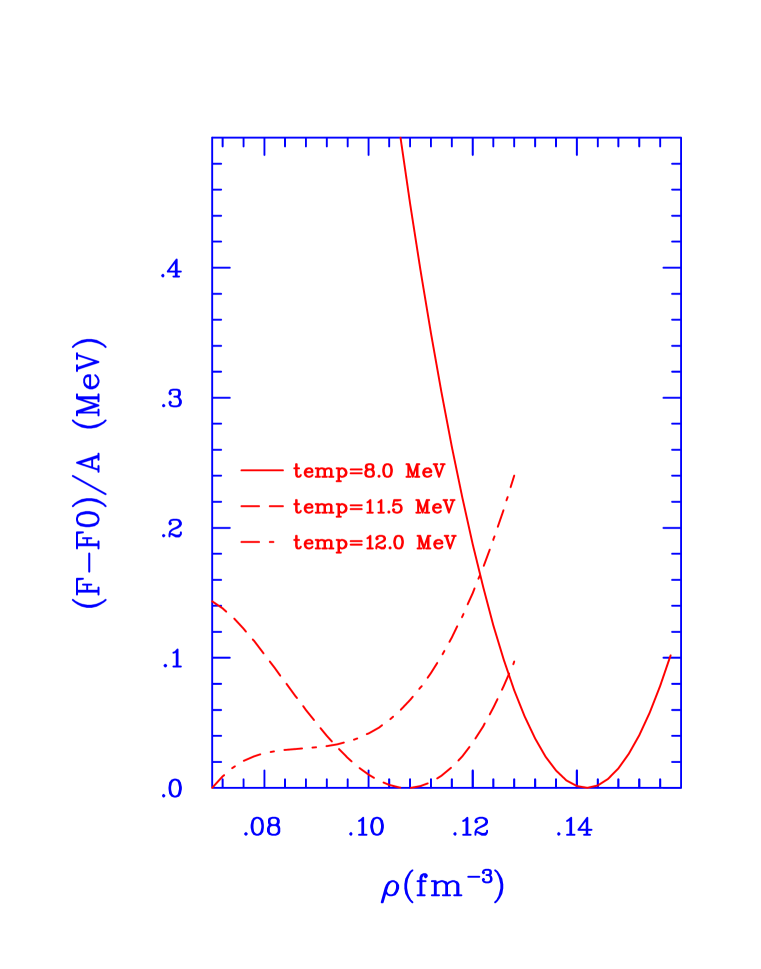
FIG. 1.: The free energy per particle as function of density at different temperatures. This is plotted as a difference from the minimum value of F in the frame. At temperature 12 MeV there is no minimum and the system will roll down to lower density. For this temperature already at lower values of $\rho$ in the figure, the derivative $\frac{\partial p}{\partial\rho}$ is negative, i.e., the system has entered a region of mechanical instability.

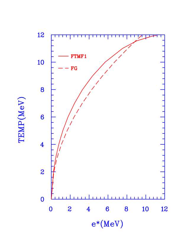
FIG. 2.: Temperature against e* in finite temperature mean field model with momentum dependence (FTMF1) and in Fermi gas model (FG). As in ref. 6, the curve with momentum dependence lies above the Fermi gas curve till they meet (around temperature 11.5 MeV). Beyond the FTMF1 curve flattens. Just below temperature 12 MeV the curve stops. The nucleus will break up into many pieces at higher temperature.

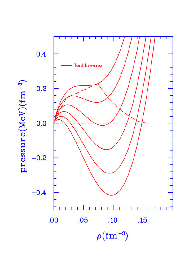
FIG. 3.: Isotherms at temperatures 6, 8, 10, 12, 14 and 15.64 MeV in mean field model with density dependence but no momentum dependence. The dashed line is the co-existence line. Also shown is the $p$=0 line. The intersections of this line with the isotherms give the the minima (in the high density side) and maxima (in the low density side) of free energy.

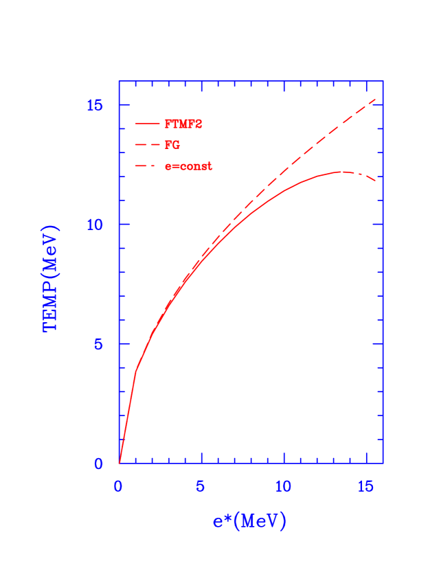
FIG. 4.: The caloric curve according to finite temperature mean field theory (solid curve), according to finite excitation mean field theory and $e^{*}=aT^{2}$ Fermi-gas approximation (dashed curve). The finite temperature and finite excitation answers are the same upto $e^{*}\approx$13.6 MeV. The finite temperature model stops here with zero slope for $T$. The finite excitation model continues beyond but with an unphysical negative slope for $T$. This part belongs to the negative compressibility zone of Fig.3.

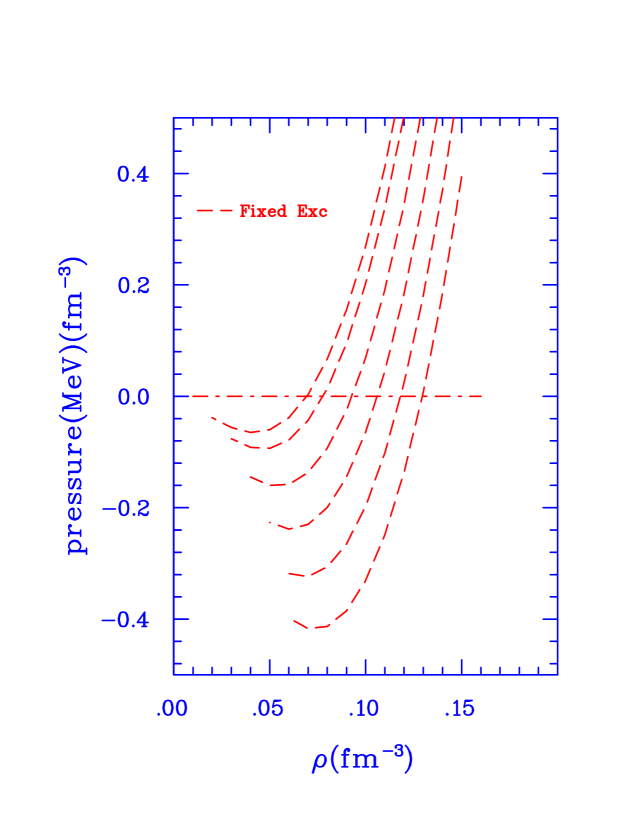
FIG. 5.: Pressure against $\rho$ curves for fixed excitation energies which in this case are, starting from the lowest, for $e^{*}$= 6, 8, 10, 12, 14 and 15 MeV. The curves terminate on the low density side when the energy cost of expansion equals $e^{*}$. The curves intersect the $p$=0 line at only one point unlike the case for isotherms (Fig.3).

REFERENCES

- [1] S. Das Gupta, A. Z. Mekjian and M. B. Tsang, Advances in Nuclear Physics, vol.26, 91 (2001)
- [2] J. P. Bondorf, R. Donangelo, I. M. Mishustin, and H. Schulz, Nucl. Phys. A444,321 (1985)
- [3] J. Pochodzalla et al., Phys. Rev. Lett. 75, 1040 (1995)
- [4] C. B. Das, S. Das Gupta, W. G. Lynch, A. Z. Mekjian, and M. B. Tsang, Phys. Rep. 406, 1, (2005)
- [5] G. F. Bertsch and S. Das Gupta, Phys. Rep. 160, 189 (1988)
- [6] L. G. Sobotka, R. J. Charity, J. Toke and W. U. Schroder, Phys. Rev. Lett. 93 ,132702 (2004)
- [7] J. Toke, J. Lu and W. Udo Schroder, Phys. Rev. Cbf 67, 034609 (2003)
- [8] N. H. March, W. H. Young and S. Sampanther, The Many-Body problem in Quantum Mechanics,(Cambridge University Press, Cambridge, 1967)p. 243
- [9] J. N. De, S. Das Gupta, S. Shlomo, and S. K. Samaddar, Phys. Rev C55,R1641 (1997)
- [10] G. M. Welke, M. Prakash, T.T. S. Kuo, S. Das Gupta, and C. Gale, Phys. Rev. C38, 2101 (1988)
- [11] C. Gale, G. M. Welke, M. Prakash, S. J. Lee and S. Das Gupta, Phys. Rev. C41, 1545 (1990)
- [12] J. Zhang, S. Das Gupta and C. Gale, Phys. Rev. C50, 1617 (1994)
- [13] S. Das Gupta, nucl-th/0412057 v1,15 Dec.,(2004)
- [14] L. Sobotka, private communication.
- [15] C. Mahaux, P. F. Bortignon, R. A. Broglia and C. H. Dasso, Phys. Rep. 120, 1 (1985)
- [16] F. Reif, Fundamentals of statistical and thermal physics(McGraw Hill, New York, 1965)Chapter 8.
- [17] A. Bohr and B. R. Mottelson, Nuclear Structure, Vol.1 (W. A. Benjamin Inc, New York, 1969)Appendix 2B