Renormalization of NN Interaction with Chiral Two Pion Exchange Potential. Non-Central Phases.

Abstract

We extend the renormalization of the NN interaction with Chiral Two Pion Exchange Potential to the calculation of non-central partial wave phase shifts with total angular momentum $j\leq 5$. The short distance singularity structure of the potential as well as the requirement of orthogonality conditions on the wave functions determines exactly the number of undetermined parameters after renormalization.

I Introduction

The original proposal by Weinberg Weinberg:1990rz ; Weinberg:1991um and carried out for the first time by Ray, Ordoñez and van Kolck Ordonez:1995rz , of making model independent predictions for NN scattering using Chiral Perturbation Theory (ChPT) has been followed by a wealth of works  Rijken:1995pu ; Kaiser:1997mw ; Kaiser:1998wa ; Epelbaum:1998ka ; Epelbaum:1999dj ; Rentmeester:1999vw ; Friar:1999sj ; Richardson:1999hj ; Kaiser:1999ff ; Kaiser:1999jg ; Kaiser:2001at ; Kaiser:2001pc ; Kaiser:2001dm ; Entem:2001cg ; Entem:2002sf ; Rentmeester:2003mf ; Epelbaum:2003gr ; Epelbaum:2003xx ; Entem:2003cs ; Higa:2003jk ; Higa:2003sz ; Higa:2004cr ; Birse:2003nz ; Entem:2003ft ; Epelbaum:2004fk (for a review see e.g. Ref. Bedaque:2002mn ). The renormalized potential as given in Refs. Ordonez:1995rz ; Kaiser:1997mw ; Rentmeester:1999vw in configuration space is expanded taking $m^{2}/16\pi^{2}f^{2}$ and $m/M$ as small parameters ($m$ and $M$ are the pion and nucleon masses respectively and $f$ is the pion weak decay constant), with $mr$ fixed. In this counting for the potential and in a given partial wave (coupled) channel with good total angular momentum the reduced potential can schematically be written as

$$U(r) = Mm\Big{\{}\frac{m^{2}}{f^{2}}W^{(0)}(mr)+\frac{m^{4}}{f^{4}}W^{(2)}(mr)$$ (1)

$$+ \frac{m^{4}}{f^{4}}\frac{m}{M}W^{(3)}(mr)+\dots\Big{\}}\,,$$

where $W^{(n)}$ are known dimensionless functions which are everywhere finite except for the origin and depend on the axial coupling constant. $W^{(3)}$ depends also on three additional low energy constants $\bar{c}_{1}=c_{1}M$, $\bar{c}_{3}=c_{3}M$ and $\bar{c}_{4}=c_{4}M$ which have been determined from $\pi N$ scattering ChPT studies in a number of works Fettes:1998ud ; Buettiker:1999ap ; GomezNicola:2000wk ; Nicola:2003zi .

At the level of approximation of Eq. (1) these potentials are local and energy independent and become singular at the origin. Thus, non-perturbative renormalization methods must be applied to give a precise meaning to the scattering amplitude Case:1950 (for a comprehensive review in the one channel case see e.g. Ref. Frank:1971 and Ref. Beane:2000wh for a modern perspective). Several methods have been proposed to study the LO term in Eq. (1) for central Frederico:1999ps ; Beane:2001bc ; PavonValderrama:2003np ; PavonValderrama:2004nb ; PavonValderrama:2005gu and non-central Nogga:2005hy waves. Recently PavonValderrama:2005gu ; Valderrama:2005wv we have shown how a renormalization program can be carried out for the NN interaction for the One Pion Exchange (OPE) and chiral Two Pion Exchange (TPE) potentials in the central ${}^{1}S_{0}$ and ${}^{3}S_{1}-^{3}D_{1}$ waves and its implications for the deuteron and pion-deuteron scattering Valderrama:2006np . In the present work we extend our analysis to all remaining partial waves with $j\leq 5$ both for the OPE as well as for the chiral TPE potentials. As we showed in Refs. PavonValderrama:2005gu ; Valderrama:2005wv the short distance behaviour of the chiral NN potential, Eq. (1), determines exactly how many counterterms are needed in order to generate renormalized and finite, i.e. cut-off independent, phase shifts. These counterterms can be determined by fixing some low energy parameters while the cut-off is removed. It has been assumed that dimensional power counting in the counterterms can be made independently on the short distance singularity of the potential. This yields conflicts between naive dimensional power counting and renormalization which have been reported recently even for low partial waves Nogga:2005hy . So, one is led to an alternative: either one keeps the power counting and a finite cut-off or one removes the cut-off at the expense of modifying the power counting of the short distance interaction. The finite cut-off route has been explored in great detail in the past Rentmeester:1999vw ; Epelbaum:1999dj ; Epelbaum:2003gr ; Epelbaum:2003xx ; Entem:2003ft ; Rentmeester:2003mf . In this paper we explore further the possibility of taking the alternative suggested by renormalization and the tight constraints imposed by finiteness. The analysis becomes rather transparent in coordinate space, where the counterterms can be mapped into boundary conditions PavonValderrama:2003np ; PavonValderrama:2004nb ; PavonValderrama:2004td at the origin. In practice renormalization may be carried out in several ways. In coordinate space it seems natural to exploit the locality of the long distance (renormalized) potentials and then to renormalize the full scattering problem. In the present work we adhere to this two-steps renormalization which has the additional advantage of making possible to determine a priori and based on simple analytical arguments the existence of the renormalized limit and how many independent renormalization conditions (counterterms) are compatible with this limit. In this regard, let us remind that the main advantage of renormalization is that identical finite and unique results should be obtained regardless of the method of calculation (coordinate or momentum space) and regularization provided the same input physical data are used to eliminate the divergencies. In particular we also expect independence on the way how the limit is taken.

The origin of the conflict can be traced back to the question whether for a given energy independent local potential, such as Eq. (1), one can assume any short distance physics regardless on the form of the long range potential. Renormalization group invariance, however, requires that any physical parameter sits on a renormalization trajectory and the corresponding evolution on the renormalization scale is dictated by the form of the long distance potential at all distances. The precise trajectory is uniquely fixed by a renormalization condition at very long distances. Thus, the separation between the short and long distance contribution is not only scale dependent but also potential dependent PavonValderrama:2003np ; PavonValderrama:2004nb . Renormalization conditions are physical and do not exhibit this dependence. Finiteness of the scattering amplitude and orthogonality of scattering (and eventually bound state) wave functions impose very tight constraints on the allowed number of counterterms and their possible scale dependence PavonValderrama:2005gu ; Valderrama:2005wv . The discussion becomes rather straightforward in coordinate space and in terms of boundary conditions for ordinary differential equations. In addition, unlike momentum space treatments, a very natural hierarchy of the renormalization problem takes place in configuration space  PavonValderrama:2005gu ; Valderrama:2005wv . More specifically, orthogonality of different energy solutions requires an energy independent boundary condition on the wave function for the long distance local and energy independent potentials as it is the case for Eq. (1) valid to NNLO, so that in all cases the effective range, and higher order threshold parameters cannot be taken as independent input parameters .

The results found in Refs. PavonValderrama:2005gu ; Valderrama:2005wv can be concisely summarized as follows in the one channel case. For a regular potential, i.e., diverging less strongly than the inverse square potential, $r^{2}|U(r)|<\infty$, one may choose between the regular and irregular solution. In the first case the scattering length is predicted while in the second case the scattering length becomes an input of the calculation. Singular potentials at the origin, i.e. fulfilling, $r^{2}|U(r)|\to\infty$, do not allow this choice. If the potential is repulsive, the scattering length depends on the potential while for an attractive potential the scattering length must be chosen as an independent parameter. In the coupled channel situation one must look at the strongest singularity of the potential eigenvalues at the origin, and apply the single channel results.

In our formulation of the NN renormalization problem threshold parameters play an essential role. Unfortunately, scattering threshold parameters for higher partial waves other than the S-waves have never been considered in the context of chiral potentials Rentmeester:1999vw ; Epelbaum:1999dj ; Epelbaum:2003gr ; Epelbaum:2003xx ; Entem:2003ft ; Rentmeester:2003mf . Instead, some calculations adjust their counterterms to fit the phase shifts in the region above threshold to the Nijmegen database Stoks:1993tb ; Stoks:1994wp . In a recent work we have filled the gap by carrying out a complete determination of these threshold parameters for the Reid93 and NijmII potentials PavonValderrama:2004se . On the light of this new information it is quite possible that the good fits in the intermediate energy region imply a somewhat less accurate description in the threshold region. This issue will become relevant in the description of some partial waves.

The paper is organized as follows. In Sect. II we review the formalism for coupled channel scattering in the presence of singular potentials at the origin. For completeness we list the potentials in Appendix A. Based on the short distance behaviour of those potentials (see Appendix C) and the requirement of orthogonality we determine the number of independent parameters for any partial wave with $j\leq 5$. In Sect. III we present our results for the phase shifts. Specifically, we make a thorough analysis of cut-off dependence in all partial waves both for the OPE as well as for the chiral TPE potential. We also discuss the perturbative nature of peripheral waves within the present non-perturbative approach. Finally, in Sect. IV we present our conclusions.

II Formalism

We solve the coupled channel Schrödinger equation for the relative motion which in compact notation reads,

$$-{\bf u}^{\prime\prime}(r)+\left[{\bf U}(r)+\frac{{\bf l}^{2}}{r^{2}}\right]{\bf u}(r)=k^{2}{\bf u}(r)\,,$$ (2)

where ${\bf U}(r)=2\mu_{np}{\bf V}(r)$ is the coupled channel matrix reduced potential with $\mu_{np}=M_{p}M_{n}/(M_{p}+M_{n})$ the reduced proton-neutron mass which for $j>0$ can be written as,

$${\bf U}^{0j}(r) = U_{jj}^{0j}\,,$$

$${\bf U}^{1j}(r) = \begin{pmatrix}U_{j-1,j-1}^{1j}(r)&0&U_{j-1,j+1}^{1j}(r)\\ 0&U_{jj}^{1j}(r)&0\\ U_{j-1,j+1}^{1j}(r)&0&U_{j+1,j+1}^{1j}(r)\end{pmatrix}\,.$$

In Eq. (2) ${\bf l}^{2}={\rm diag}(l_{1}(l_{1}+1),\dots,l_{N}(l_{N}+1))$ is the orbital angular momentum, ${\bf u}(r)$ is the reduced matrix wave function, $k$ the C.M. momentum and $j$ the total angular momentum. In our case $N=1$ for the spin singlet channel with $l=j$ and $N=3$ for the spin triplet channel with $l_{1}=j-1$, $l_{2}=j$ and $l_{3}=j+1$. The potentials used in this paper were obtained in Refs. Ordonez:1995rz ; Kaiser:1997mw ; Rentmeester:1999vw in coordinate space and are listed in Appendix A for completeness.

II.1 Long distance behaviour

At long distances, we assume the usual asymptotic normalization condition

$${\bf u}(r)\to\hat{\bf h}^{(-)}(r)-\hat{\bf h}^{(+)}(r){\bf S}\,,$$ (4)

with ${\bf S}$ the coupled channel unitary S-matrix. The corresponding out-going and in-going free spherical waves are given by

$$\hat{\bf h}^{(\pm)}(r) = {\rm diag}(\hat{h}^{\pm}_{l_{1}}(kr),\dots,\hat{h}^{\pm}_{l_{N}}(kr))\,,$$ (5)

with $\hat{h}^{\pm}_{l}(x)$ the reduced Hankel functions of order $l$, $\hat{h}_{l}^{\pm}(x)=xH_{l+1/2}^{\pm}(x)$ ( $\hat{h}_{0}^{\pm}(x)=e^{\pm ix}$ ), and satisfy the free Schrödinger’s equation for a free particle.

For the spin singlet state, $s=0$, one has $l=j$ and hence the state is uncoupled

$$S_{jj}^{0j}=e^{2i\delta_{j}^{0j}}\,,$$ (6)

whereas for the spin triplet state $s=1$, one has the uncoupled $l=j$ state

$$S_{jj}^{1j} = e^{2i\delta_{j}^{1j}}\,,$$ (7)

and the two channel coupled $l,l^{\prime}=j\pm 1$ states for which we use Stapp-Ypsilantis-Metropolis (SYM or Nuclear bar) stapp parameterization

$$S^{1j} = \left(\begin{array}[]{cc}S_{j-1\,j-1}^{1j}&S_{j-1\,j+1}^{1j}\\ S_{j+1\,j-1}^{1j}&S_{j+1\,j+1}^{1j}\end{array}\right)$$ (10)

$$= \left(\begin{array}[]{cc}\cos{(2\bar{\epsilon}_{j})}e^{2i\bar{\delta}^{1j}_{j-1}}&i\sin{(2\bar{\epsilon}_{j})}e^{i(\bar{\delta}^{1j}_{j-1}+\bar{\delta}^{1j}_{j+1})}\\ i\sin{(2\bar{\epsilon}_{j})}e^{i(\bar{\delta}^{1j}_{j-1}+\bar{\delta}^{1j}_{j+1})}&\cos{(2\bar{\epsilon}_{j})}e^{2i\bar{\delta}^{1j}_{j+1}}\end{array}\right)$$ (13)

In the discussion of low energy properties we also use the Blatt-Biedenharn (BB or Eigen phase) parameterization Bl52 defined by

$$S^{1j} = \begin{pmatrix}\cos\epsilon_{j}&-\sin\epsilon_{j}\\ \sin\epsilon_{j}&\cos\epsilon_{j}\end{pmatrix}\begin{pmatrix}e^{2{\rm i}\delta^{1j}_{j-1}}&0\\ 0&e^{2{\rm i}\delta_{j+1}^{1j}}\end{pmatrix}$$ (14)

$$\times \begin{pmatrix}\cos\epsilon_{j}&\sin\epsilon_{j}\\ -\sin\epsilon_{j}&\cos\epsilon_{j}\end{pmatrix}\,.$$

The relation between the BB and SYM phase shifts is

$$\bar{\delta}_{j+1}^{1j}+\bar{\delta}_{j-1}^{1j} = \delta_{j+1}^{1j}+\delta_{j-1}^{1j}\,,$$ (15)

$$\sin(\bar{\delta}_{j-1}^{1j}-\bar{\delta}_{j+1}^{1j}) = \frac{\tan(2\bar{\epsilon}_{j})}{\tan(2\epsilon_{j})}\,.$$ (16)

In the present paper zero energy scattering parameters play an essential role since they are often used (see below) as input parameters of the calculation of phase shifts. Due to unitarity of the S-matrix in the low energy limit, $k\to 0$, we have

$$\left({\bf S}-{\bf 1}\right)_{l^{\prime},l}=-2{\rm i}\alpha_{l^{\prime},l}k^{l^{\prime}+l+1}+\dots\,,$$ (17)

with $\alpha_{l^{\prime}l}$ the (hermitian) scattering length matrix . The threshold behaviour acquires its simplest form in the SYM representation,

$$\delta^{0j}_{j} \to -\alpha^{0j}_{j}k^{2j+1}\,,$$ (18)

$$\delta^{1j}_{j} \to -\alpha^{1j}_{j}k^{2j+1}\,,$$ (19)

$$\bar{\delta}^{1j}_{j-1} \to -\bar{\alpha}^{1j}_{j-1}k^{2j-1}\,,$$ (20)

$$\bar{\delta}^{1j}_{j+1} \to -\bar{\alpha}^{1j}_{j+1}k^{2j+3}\,,$$ (21)

$$\bar{\epsilon}_{j} \to -\bar{\alpha}^{1j}_{j}k^{2j+1}\,.$$ (22)

In the BB form one has similar behaviours for the $\delta$’s but for $\epsilon_{j}$ which behaves as $k^{2j}$ instead of $k^{2j+1}$

$$\delta^{1j}_{j-1} \to -\bar{\alpha}^{1j}_{j-1}\,k^{2j-1}\,,$$ (23)

$$\delta^{1j}_{j+1} \to -(\bar{\alpha}^{1j}_{j+1}-\frac{{({\bar{\alpha}}^{1j}_{j})}^{2}}{\bar{\alpha}^{1j}_{j-1}})\,k^{2j+3}\,,$$ (24)

$$\epsilon_{j} \to \frac{\bar{\alpha}^{1j}_{j}}{\bar{\alpha}^{1j}_{j-1}}\,k^{2j}\,.$$ (25)

II.2 Short distance behaviour

The form of the wave functions at the origin is uniquely determined by the form of the potential at short distances (see e.g. Case:1950 ; Frank:1971 for the case of one channel and PavonValderrama:2005gu ; Valderrama:2005wv for coupled channels). For the chiral NN potential, Eq. (1), one has

$${\bf U}_{\rm LO}(r) \to \frac{M{\bf C}_{3,LO}}{r^{3}}\,,$$

$${\bf U}_{\rm NLO}(r) \to \frac{M{\bf C}_{5,NLO}}{r^{5}}\,,$$

$${\bf U}_{\rm NNLO}(r) \to \frac{M{\bf C}_{6,NNLO}}{r^{6}}\,,$$

where LO includes the first term in Eq. (1), NLO the first two terms and so on. Note that higher order potentials become increasingly singular at the origin. For a potential diverging at the origin as an inverse power law

$${\bf U}(r)\to\frac{M{\bf C}_{n}}{r^{n}}\,,$$ (27)

with ${\bf C}_{n}$ a matrix of generalized van der Waals coefficients and $n>2$ an integer. One diagonalizes the matrix ${\bf C}_{n}$ by a constant unitary transformation, ${\bf G}$, yielding

$$M{\bf C}_{n}={\bf G}\,{\rm diag}(\pm R_{1}^{n-2},\dots,\pm R_{N}^{n-2})\,{\bf G}^{-1}\,,$$ (28)

with $R_{i}$ constants with length dimension. The plus sign corresponds to the case with a positive eigenvalue (repulsive) and the minus sign to the case of a negative eigenvalue (attractive). Then, at short distances one has the solutions

$${\bf u}(r)\to{\bf G}\begin{pmatrix}u_{1,\pm}(r)\cr\cdots\\ u_{N,\pm}(r)\end{pmatrix}\,,$$ (29)

where for the attractive and repulsive cases one has

$$u_{i,-}(r) \to C_{i,-}\left(\frac{r}{R_{i}}\right)^{n/4}\sin\left[\frac{2}{n-2}\left(\frac{R_{i}}{r}\right)^{\frac{n}{2}-1}+\varphi_{i}\right]\,,$$

$$u_{i,+}(r) \to C_{i,+}\left(\frac{r}{R_{i}}\right)^{n/4}\exp\left[-\frac{2}{n-2}\left(\frac{R_{i}}{r}\right)^{\frac{n}{2}-1}\right]\,,$$ (31)

respectively. This behaviour of the wave functions near the origin is valid regardless of the energy, provided the distances are small enough . Here, $\varphi_{i}$ are arbitrary short distance phases which in general depend on the energy. There are as many short distance phases as short distance attractive eigenpotentials. Orthogonality of the wave functions at the origin yield the relation

$$\sum_{i=1}^{N}\left[{u_{k,i}}^{*}u_{p,i}^{\prime}-{u_{k,i}^{\prime}}^{*}u_{p,i}\right]\Big{|}_{r=0}=\sum_{i=1}^{A}\cos(\varphi_{i}(k)-\varphi_{i}(p))\,,$$

where $A\leq N$ is the number of the short distance attractive eigenpotentials.

Table 1: Sets of chiral coefficients considered in this work.

Set	Source	$c_{1}({\rm GeV}^{-1})$	$c_{3}({\rm GeV}^{-1})$	$c_{4}({\rm GeV}^{-1})$
Set I	$\pi N$ Buettiker:1999ap	-0.81	-4.69	3.40
Set II	$NN$ Rentmeester:1999vw	-0.76	-5.08	4.70
Set III	$NN$ Epelbaum:2003xx	-0.81	-3.40	3.40
Set IV	$NN$ Entem:2003ft	-0.81	-3.20	5.40

The simplest choice to fix relative phases for a positive energy scattering state is to take the zero energy state $p=0$ as a reference state, and the zero energy short distance phase. In the particular case where only one eigenvalue is negative the short distance phase is energy independent. This may happen both in the singlet as well as in the triplet channels with $j=l$. The short distance phase is then fixed by reproducing the scattering length in the singlet channel and one of the three scattering lengths in the triplet channel. In the case where one has two negative, i.e. attractive, eigenvalues (this can only happen in triplet channels) there are two undetermined short distance phases which can be fixed by using the corresponding three scattering lengths. The case of two positive, i.e. repulsive, eigenvalues does not allow to fix any scattering length. The case with two different signs for the eigenvalues fixes one scattering length only. Note that in this construction and for two coupled channels there is no intermediate situation where the solution is specified by just two scattering lengths; one has either zero, one or three.

Although our arguments are entirely based on analytical calculations, one should mention that our conclusions are in agreement with the findings of Ref. Nogga:2005hy for the OPE case. There, counterterms beyond the ones dictated by Weinberg’s power counting are included in the ${}^{3}P_{0}$, ${}^{3}P_{2}-{}^{3}F_{2}$ and ${}^{3}D_{2}$ waves to ensure renormalizability on numerical grounds. As we will see below, our renormalized phase shifts for special case OPE reproduce essentially their results, although our TPE non-perturbatively renormalized amplitudes go beyond these results.

Another issue is that of the establishment of a theoretically compelling and mathematically consistent power counting which also provides phenomenological success. This has been the goal of much the EFT activity in recent years. Despite the fact that our OPE is mathematically identical to the one in Ref. Nogga:2005hy where a strong emphasis on power counting has been made, our motivation is slightly different. Actually, these authors argue that a consistent scheme for TPE might be achieved within a perturbative framework, using the non-perturbative OPE distorted amplitudes as the leading order approximation. This is theoretically appealing and the issue was thoroughly discussed within the coordinate space approach in our previous paper on the central waves Valderrama:2005wv . There, it was pointed out that with enough counterterms such a program could be pursued although orthogonality was violated and results did not exhibit a clear improvement as compared to the fully iterated potentials. The reason was the appearance of non-analytical dependences on the would-be dimensional power counting parameter, a situation that has not been foreseen in the standard EFT set up. This suggests that discussion on power counting and the systematics of EFT is not yet over. Therefore, and as we did in our previous work, we focus more on establishing long range model independent correlations, leaving the possible establishment of a satisfactory power counting for future studies.

II.3 Regularization methods

In principle, it is possible to implement the short distance behaviour of the wave functions, Eq. (31), if one goes to sufficiently small distances, or if the short distance behaviour of the the wave function is improved PavonValderrama:2005gu . Computationally, the implementation of short distance regulators is mostly straightforward. The attractive or repulsive nature of the potentials at short distances requires different choices of regulators PavonValderrama:2005gu ; Valderrama:2005wv . For a one-channel repulsive singular potential we use the regulator

$$\frac{u_{k}^{\prime}(a)}{u_{k}(a)}=\frac{l+1}{a}\,,$$ (33)

This condition ensures orthogonality of wave functions with different energy. For the attractive singular case, we integrate in from infinity at zero energy down to a given boundary radius, $a$, impose orthogonality at the boundary by matching logarithmic derivatives

$$\frac{u_{k}^{\prime}(a)}{u_{k}(a)}=\frac{u_{0}^{\prime}(a)}{u_{0}(a)}\,,$$ (34)

and then integrate out at finite energy. In the coupled channel case we extend the method by applying the one channel regularization to the short distance eigen functions, Eq. (29).

II.4 Fixing of parameters and renormalization conditions

Fixing of the short distance phases requires some renormalization condition. As we have said, an appealing choice is to impose this condition at zero energy. The way to proceed in practice is quite straightforward, although tedious given the large number (27) of partial waves considered in this work. In the singlet channel case and for an attractive short distance singularity, one starts at zero energy and integrates in from large distances $\sim 15{\rm fm}$ with a given scattering length until a short boundary radius $\sim 0.1{\rm fm}$. At finite energy one integrates out matching the wave function to the zero energy solution at the short distance boundary generating a phase shift from a given prescribed scattering length. Of course, in this method one has to check for cut-off independence (taking $r=0.1-0.2{\rm fm}$ proves enough). For the coupled channel case one proceeds along similar lines and the procedure has been described in great detail in our previous works PavonValderrama:2005gu ; Valderrama:2005wv for the $j=1$ channel. The method relies heavily on the superposition principle of boundary conditions and we use here the extension of that method to higher partial waves. One of the advantages of our approach is that we rarely have to make a fit to the data; any phase shift has by construction the right threshold behaviour in the case where the potential at short distances is attractive. For the repulsive potential case the scattering length is predicted entirely from the potential. In any case, discrepancies with the data can be attributed to the potential.

Table 2: The number of independent parameters for different orders of approximation of the potential. The scattering lengths are in ${\rm fm}^{l+l^{\prime}+1}$ and are taken from NijmII and Reid93 potentials Stoks:1994wp in Ref. PavonValderrama:2004se . We use the (SYM-nuclear bar) convention, Eq. (22).

Wave	$\alpha$ NijmII (Reid93)	LO	NLO	NNLO
${}^{1}S_{0}$	-23.727(-23.735)	Input	Input	Input
${}^{3}P_{0}$	-2.468(-2.469)	Input	—	Input
${}^{1}P_{1}$	2.797(2.736)	—	—	—
${}^{3}P_{1}$	1.529(1.530)	—	Input	Input
${}^{3}S_{1}$	5.418(5.422)	Input	—	Input
${}^{3}D_{1}$	6.505(6.453)	—	—	Input
$E_{1}$	1.647(1.645)	—	—	Input
${}^{1}D_{2}$	-1.389(-1.377)	—	Input	Input
${}^{3}D_{2}$	-7.405(-7.411)	Input	Input	Input
${}^{3}P_{2}$	-0.2844(-0.2892)	Input	Input	—
${}^{3}F_{2}$	-0.9763(-0.9698)	—	—	—
$E_{2}$	1.609(1.600)	—	—	—
${}^{1}F_{3}$	8.383(8.365)	—	—	—
${}^{3}F_{3}$	2.703(2.686)	—	Input	Input
${}^{3}D_{3}$	-0.1449(-0.1770)	Input	—	Input
${}^{3}G_{3}$	4.880(4.874)	—	—	Input
$E_{3}$	-9.695(-9.683)	—	—	Input
${}^{1}G_{4}$	-3.229(-3.210)	—	Input	Input
${}^{3}G_{4}$	-19.17(-19.14)	Input	Input	Input
${}^{3}F_{4}$	-0.01045(-0.01053)	Input	Input	—
${}^{3}H_{4}$	-1.250(-1.240)	—	—	—
$E_{4}$	3.609(3.586)	—	—	—
${}^{1}H_{5}$	28.61(28.57)	—	—	—
${}^{3}H_{5}$	6.128(6.082)	—	Input	Input
${}^{3}G_{5}$	-0.0090(-0.010)	Input	—	Input
${}^{3}I_{5}$	10.68(10.66)	—	—	Input
$E_{5}$	-31.34(-31.29)	—	—	Input

Inspection of Table 2 illustrates the situation for the LO, NLO, and NNLO approximations to the potential. We show the scattering lengths in all partial waves as determined in our previous work PavonValderrama:2004se together with the corresponding eigenvalues for the leading short distance coefficients in the LO (OPE), NLO and NNLO approximations to the potential. In the NNLO one must also specify the values of the chiral constants $c_{1}$, $c_{3}$ and $c_{4}$. We use for definiteness the values of Ref. Entem:2003ft , since as we saw in Ref. Valderrama:2005wv they provide a reasonable description of deuteron properties.

II.5 Details on the numerical procedure

The integration of the coupled differential equations requires some care, particularly in the vicinity of the short distance singularities. In the case of attractive singularities due to the increasing oscillations the wave function has to be sampled with great detail at a rate similar to the size of the oscillations. For the repulsive case, one must stop at sufficiently large distances due to the exponential suppression of the wave function. Another important condition has to do with preservation of in and out reversibility of the integration. This last requirement guarantees that for attractive channels, where the scattering length is supplied as an input parameter, the threshold behaviour of the phase shift is consistent with that given scattering length.

Another problem one has to face for high partial waves is related to the practical influence of the scattering length on the calculated phase shifts. In principle, and for an attractive singular potential, the scattering length needs to be specified. For the one channel case, this is done by integrating in the zero energy large distance solution, valid for $r\gg 2/m_{\pi}$

$$u(r)\to r^{-l}-\frac{r^{l+1}}{\alpha_{l}}\,,$$ (35)

The long distance irregular solution dominates, unless $\alpha_{l}$ is anomalously large , i.e. $\alpha_{l}(m_{\pi}/2)^{(2l+1)}\gg 1$ , so that when integrating in much of the regular solution will be lost and the result will be rather insensitive to the value of $\alpha_{l}$ provided it is of normal size. This fact becomes relevant in the numerical calculations if the long distance cut-off is taken to be exceedingly large. To avoid this situation we take typically $R_{\rm max}=15{\rm fm}$ for large $l$.

Table 3: Deuteron properties for the OPE and TPE potentials. OPE(0) refers to the deuteron computed by orthogonality to the zero energy scattering states, fixing $\alpha_{0}$ to its experimental value, while in OPE(B) the computation is made by fixing $\gamma$ to its experimental value, constructing the corresponding bound state. Similarly, TPE(0) refers to the deuteron computed by orthogonality to zero energy states, fixing $\alpha_{0}$ to its experimental value and $\alpha_{02}$ and $\alpha_{2}$ to their Nijmegen II values, while in TPE(B) the computation is made by fixing $\gamma$, $\eta$ and $\alpha_{0}$ to their experimental values. The errors quoted in OPE(0) corresponds to the uncertainty in the value of the scattering length, while in OPE(B) the errors correspond to changing the cutoff in the $0.1-0.2\,{\rm fm}$ range. The errors quoted in both TPE computations reflect the uncertainty in the non-potential parameters $\gamma$, $\eta$ and $\alpha_{0}$ only. We take set IV Entem:2003ft for the LEC’s in the TPE calculation. Experimental values can be traced from Ref. deSwart:1995ui .

Set	$\gamma\,\,({\rm fm}^{-1})$	$\eta$	$A_{S}\,\,({\rm fm}^{-1/2})$	$r_{m}\,\,({\rm fm})$	$Q_{d}({\rm fm}^{2})$	$P_{D}$ (%)	$\alpha_{0}\,({\rm fm})$	$\alpha_{02}({\rm fm}^{3})$	$\alpha_{2}({\rm fm}^{5})$
OPE(0)	0.2274(4)	0.02564(4)	0.8568(10)	1.964(3)	0.2796(3)	7.208(12)	Input	1.754(7)	6.770(7)
OPE(B)	Input	0.02633	0.8681(1)	1.9351(5)	0.2762(1)	7.31(1)	5.335(1)	1.673(1)	6.693(1)
TPE(0)	0.2322(3)	0.02531(9)	0.8891(4)	1.968(3)	0.2723(3)	7.24(13)	Input	NijmII	NijmII
TPE(B)	Input	Input	0.884(4)	1.967(6)	0.276(3)	8(1)	Input	1.67(4)	6.6(4)
NijmII	0.231605	0.02521	0.8845	1.9675	0.2707	5.635	5.418	1.647	6.505
Reid93	0.231605	0.02514	0.8845	1.9686	0.2703	5.699	5.422	1.645	6.453
Exp.	0.231605	0.0256(4)	0.8846(9)	1.971(6)	0.2859(3)	-	5.419(7)	-	-

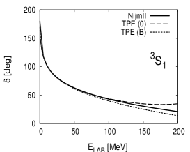
Figure 1: Dependence of the ${}^{3}S_{1}-^{3}D_{1}$ channel (SYM-nuclear bar) phase shifts for the NNLO TPE potential on the reference state used to orthogonalize the scattering state compared to the corresponding phases of the database of Ref. Stoks:1993tb ; Stoks:1994wp . Label TPE(0) means the zero energy reference state with $\alpha_{0}=5.418{\rm fm}$, $\alpha_{02}=1.647{\rm fm}^{3}$ and $\alpha_{2}=6.505{\rm fm}^{5}$. Label TPE(B)stands for the deuteron bound reference state with the experimental binding energy, asymptotic $D/S$ ratio together with $\alpha_{0}=5.418{\rm fm}$ (corresponding to $\alpha_{02}=1.67\,{\rm fm}^{3}$ and $\alpha_{2}=6.6\,{\rm fm}^{5}$ Valderrama:2005wv .)

Figure 2: np (SYM-nuclear bar) Phase shifts for the total angular momentum $j=0$. OPE (left) and chiral TPE (middle) as a function of the cut-off radius $R_{S}$ for fixed LAB energies, $E_{\rm LAB}=10,50,100{\rm MeV}$. OPE and chiral TPE (left) renormalized (i.e. $R_{S}\to 0$) phase shifts as a function of the LAB energy compared to the Nijmegen partial wave analysis Stoks:1993tb ; Stoks:1994wp .

Figure 3: Same as Fig. 2 but for $j=1$.

Figure 4: Same as Fig. 2 but for $j=2$.

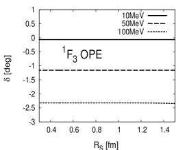
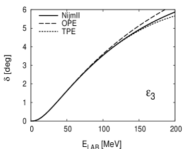
Figure 5: Same as Fig. 2 but for $j=3$.

Figure 6: Same as Fig. 2 but for $j=4$.

Figure 7: Same as Fig. 2 but for $j=5$.

III Results for the Phase Shifts

III.1 Numerical parameters

For our numerical calculations we take $f_{\pi}=92.4{\rm MeV}$, $m=138.03{\rm MeV}$, $2\mu_{np}=M=M_{p}M_{n}/(M_{p}+M_{n})=938.918{\rm MeV}$, $g_{A}=1.29$ in the OPE piece to account for the Goldberger-Treimann discrepancy and $g_{A}=1.26$ in the TPE piece of the potential. The corresponding pion nucleon coupling constant takes then the value $g_{\pi NN}=13.083$ (i.e. $g_{A}=1.29$) according to the Nijmegen phase shift analysis of NN scattering deSwart:1997ep . The values of the coefficients $c_{1}$, $c_{3}$ and $c_{4}$ used along this paper can be looked up in Table 1 for completeness. The potentials in configuration space used in this paper are exactly those provided in Ref. Ordonez:1995rz ; Kaiser:1997mw ; Rentmeester:1999vw but disregarding relativistic corrections, $M/E\to 1$ . The potentials are listed in Appendix A for completeness. The short distance van der Waals coefficients for all channels studied in the present work are presented in Appendix C. The output of such a channel by channel analysis is briefly summarized in Table 2 where we indicate which scattering lengths are used as input parameters according to the discussion given in Sect. II. Low energy parameters for the high quality potentials Stoks:1993tb ; Stoks:1994wp have been obtained in Ref. PavonValderrama:2004se . We will use the Nijm II values, but to give an idea on the expected lower uncertainties on those parameters we also list the Reid93 values. Probably the real uncertainties are much larger since the actual value of these low energy parameter will depend upon which long range physics is included in the high quality potentials where explicit TPE effects have not been included, as we do in the present work .

III.2 The deuteron channel revisited

Before embarking in the full fledged discussion of all partial waves, it is interesting to reanalyze first the ${}^{3}S_{1}-^{3}D_{1}$ channel already studied in our previous work on the deuteron PavonValderrama:2005gu ; Valderrama:2005wv . There, we used the orthogonality to the deuteron bound state. The scattering lengths $\alpha_{02}=1.67\,{\rm fm}^{3}$ and $\alpha_{2}=6.6\,{\rm fm}^{5}$ were deduced from the experimental deuteron binding energy, the asymptotic $D/S$ ratio and the S-wave scattering length $\alpha_{0}$. These values turned out to be a bit off the values deduced from the NijmII and Reid93 potentials PavonValderrama:2004td (see Table 2). Nevertheless, the intermediate energy region turned out to be better described than the low energy behaviour suggested. In the present work we choose instead to build scattering states which are orthogonal to the zero energy states, so deuteron properties can be deduced, as done in table 3. In Fig. 1 we show the results when either the zero energy or the deuteron bound state are used as reference states. One obvious lesson from this comparison is that phase shifts, particularly the $E_{1}$ channel, may be better described in the intermediate energy region if the deuteron is used as a reference state, despite the fact that the threshold behaviour is a bit off. This is maybe explained by the observation that $\alpha_{02}$ and $\alpha_{2}$ encode higher energy information about the system than $\alpha_{0}$ or $\gamma$ , so the latter parameters are more suited to obtain an effective description of the system. This feature will become evident in other partial waves.

III.3 Cut-off dependence

In Figs. 2, 3, 4, 5, 6 and 7 we show the results of our calculation for all partial waves with $j\leq 5$ as a function of the nucleon LAB energy. For definiteness we use the chiral constants $c_{1}$, $c_{3}$ and $c_{4}$ of Ref. Entem:2003ft (Set IV) which already provided a good description of deuteron properties after renormalization Valderrama:2005wv at NNLO. This choice allows a more straightforward comparison to the N³LO calculation of Ref. Entem:2003ft with finite cut-offs. Unless otherwise stated, the needed low energy parameters for these figures are always taken to be those of Ref. PavonValderrama:2004se for the NijmII potential (see Table 2).

In order to test the stability of the phase-shifts against changes in the short distance cut-off parameter, $R_{S}$, we show in Figs. 2, 3, 4, 5, 6 and 7, and similarly to the OPE study in momentum space of Ref. Nogga:2005hy , the cut-off dependence for fixed values of the lab energy both for the OPE as well as for the TPE potentials. This is done in the range $0.15{\rm fm}\leq R_{S}\leq 1.5{\rm fm}$. If we identify this short distance cut-off with the sharp momentum cut-off $\Lambda=\pi/2R_{S}$ PavonValderrama:2004td , the smallest boundary radius, $\sim 0.15{\rm fm}$, corresponds to a maximum cut-off $\Lambda\sim 2{\rm GeV}$. This is much larger than the cut-offs used in Refs. Rentmeester:1999vw ; Epelbaum:1999dj ; Epelbaum:2003gr ; Epelbaum:2003xx ; Entem:2003ft ; Rentmeester:2003mf but comparable to the exponential cut-off used in Ref. Nogga:2005hy for the renormalization of the OPE potential  . Note that the limit $R_{S}\to 0$ may be taken independently for any different channel.

The evolution of the increasingly oscillating wave function in the attractive case can be identified with the cycles (improperly called limit-cycles, see footnote 5 in Ref. PavonValderrama:2004nb ) described in Refs. Beane:2000wh ; Beane:2001bc ; PavonValderrama:2004nb ; PavonValderrama:2004td by looking at suitable logarithmic combinations of the wave functions. The cycles documented in Ref. Nogga:2005hy in momentum space can be mapped into the coordinate space cycles by relating the coordinate and momentum space cut-offs.

Generally speaking, the inclusion of chiral TPE effects generates smoother limits as compared to the OPE results, as one would expect. We have checked that for short distance repulsive (eigen)channels results are not very sensitive to the choice of the regulator for small values of $R_{S}$. As we also see from the figures, the convergence depends both on the partial wave as well as on the energy. As expected, the needed value of the short distance cut-off $R_{S}$ for which stability is achieved is rather high for peripheral waves, $R_{S}\sim 1/m_{\pi}$. Another feature of the calculation are the observed stability plateaus for a number of partial waves. This trend has also been noted in previous works with finite cut-offs Epelbaum:2004fk where there appear sequential cut-off windows. In coordinate space this is originated by the almost self-similar pattern of the short distance oscillations of the wave function which suggest a sequential and faster convergence modulo cycles PavonValderrama:2004nb .

Let us remark at this point that the existence of an $R_{S}\to 0$ limit does not necessarily mean a plateau-like approach to it. This is the case, for example, of the ${}^{1}S_{0}$ wave, which for OPE shows a linear dependence on the cut-off due to the mild $1/r$ singularity of the potential, generating a linear-like behaviour which corresponds to the ratio of regular ($\sim r$) and irregular ($\sim 1$) solutions at the origin . A similar behaviour can be found on other singlet waves in which the OPE potential also behaves as $1/r$, but highly attenuated by the influence of the centrifugal barrier.

Finally, let us note that there are some channels where the phase shifts exhibit a very strong dependence on the regulator .

III.4 Renormalized phase shifts

III.4.1 LO (OPE)

In Figs. 2, 3, 4, 5, 6 and 7 we also compare the OPE (LO), the NNLO TPE and the Nijmegen phase shift analysis Stoks:1993tb ; Stoks:1994wp . As noted in Tab. 2 in some cases with attractive singular potentials some scattering lengths must be specified, in order to determine the phase shifts, but for repulsive singular potentials the scattering lengths and hence the phase shifts are fully determined from the potential. In the coupled channel case where only one parameter should be fixed we have chosen, as indicated in Table 2, to take the scattering length of the corresponding partial wave with the lower orbital angular momentum. As we see from Figs. 2, 3, 4, 5, 6 and 7, OPE does a relatively good job for the phases when compared to the NijmII results, up to a reasonable energy. This calculation extends our previous results PavonValderrama:2005gu using the same regularization for the singlet ${}^{1}S_{0}$ and triplet ${}^{3}S_{1}-^{3}D_{1}$ channels.

The LO results corresponding to static OPE potential have also been obtained recently in momentum space by a solution of the Lippmann-Schwinger equation in Ref. Nogga:2005hy for $j\leq 3$. These authors see that in the limit $\Lambda\to\infty$ (in practice $\Lambda=4{\rm GeV})$ it is always possible to adjust a counterterm in such a way that the phase shifts are cut-off independent. They also find that the needed counterterm does not correspond to the expectations based on Weinberg’s dimensional power counting argument, so that one is forced to promote counterterms which are of higher order in Weinberg’s counting to make the theory free of short distance ambiguities. This proposal not only fits quite naturally into our analysis of short distance boundary conditions, but can also be anticipated by just looking at the short distance behaviour of the potential. In general, we reproduce their results for the phase shifts using our boundary condition regularization (our shortest distance cut-off is typically $a=0.1{\rm fm}$ for OPE). This is precisely one of the points of renormalization; different regularization methods should yield identical results when the regulator is removed provided the same renormalization conditions are imposed. Note that in our case whenever a scattering length must be provided we exactly construct the phase shift as to reproduce the threshold behaviour of the Nijmegen phases Stoks:1993tb ; Stoks:1994wp by exactly fixing the scattering length (the renormalization condition). This requires solving the zero energy problem by integrating in with the given scattering length, and matching at short distances the finite energy problem to finally determine the phase shift by integrating out. In this approach we never make a fit. In the approach of Ref. Nogga:2005hy counterterms are adjusted to fit the phases in the region around threshold. Although this is in spirit the same renormalization condition to fix the counterterms, we expect some numerical discrepancies, due to the fact that the threshold parameters in Ref. Nogga:2005hy may be slightly different to ours.

Figure 8: Dependence of some phases for the chiral TPE potential on the scattering lengths compared to the NijmII phases Stoks:1993tb ; Stoks:1994wp . We use Set IV of chiral constants. Label TPE ($\alpha_{\rm nijm}$) means scattering lengths of Table 2 are taken as deduced in Ref. PavonValderrama:2004se , while TPE ($\alpha_{\rm tuned}$) stands for the values tuned to fit the phases in the intermediate energy region. For ${}^{3}P_{0}$ we take $\alpha_{1}=-2.670{\rm fm}^{3}$, for ${}^{3}P_{1}$ we take $\alpha_{1}=1.692{\rm fm}^{3}$ and for ${}^{1}D_{2}$ we take $\alpha_{2}=-1.666{\rm fm}^{5}$.

III.4.2 NLO (TPE)

Regarding NLO we do not show the results as they fail completely to describe the data in triplet ${}^{3}S_{1}-^{3}D_{1}$ channel. The problem we found already Valderrama:2005wv in the triplet ${}^{3}S_{1}-^{3}D_{1}$ channel persists in other channels; the short distance behaviour of the NLO potential corresponds to $1/r^{5}$ repulsive eigenpotentials. This feature explains the relatively small maximal cut-offs allowed in NLO calculations in momentum space. As stressed on our previous work there are at least two scenarios where the problem may be overcome. One possibility appeals to the role of the $\Delta$ resonance and the fact that its contribution to $c_{3}$ and $c_{4}$ scales as the inverse of the $N\Delta$ splitting $\Delta\sim 2m_{\pi}$ as found in Ref. Ordonez:1995rz ; vanKolck:1994yi ; Kaiser:1998wa . In the $\Delta$ counting the $c_{3}$ and $c_{4}$ contributions to the NNLO deltaless potential become actually NLO contributions, and the short distance behaviour becomes a $1/r^{6}$ attractive singularity. The second scenario has to do with the influence of relativity beyond a truncated heavy baryon expansion, since according to Refs. Higa:2003jk ; Higa:2003sz ; Higa:2004cr one has a relativistic $1/r^{7}$ van der Waals short distance behaviour with attractive-repulsive eigen potential meaning that as in the OPE case one has one free parameter. Calculations taking into account these effects in all partial waves are currently underway HPR2005 .

III.4.3 NNLO (chiral-TPE)

We turn now to the NNLO calculation which are the genuine predictions of ChPT because they contain the chiral constants $c_{1}$, $c_{3}$ and $c_{4}$ (see e.g. Table 1) and for definiteness we will use mainly Set IV Entem:2003ft in our analysis . Results for the TPE renormalized phase shifts are presented in Figs. 2, 3, 4, 5, 6 and 7. Some expected features do indeed occur. Peripheral waves are slightly modified by going from OPE to the chiral TPE potential. On the other hand, low partial waves are also improved in the low energy region. For instance, the ${}^{1}S_{0}$ phase has an attractive singular interaction, requiring fixing the scattering length. The difference in the curves is mainly related to the difference in the effective range which improves when going from OPE to TPE Valderrama:2005wv . This is a rather general feature, the error at low energies is controlled by the low energy threshold parameters, like the effective range and others. If one looks at the ${}^{3}P_{0}$ channel, we see that there is improvement but not as dramatic as in the ${}^{1}S_{0}$ channel.

As we have said, in singular repulsive channels, which at NNLO correspond to the ${}^{1}P_{1}$, ${}^{1}F_{3}$ and ${}^{1}H_{5}$ singlet states, and to the ${}^{3}P_{2}-{}^{3}F_{2}$ and ${}^{3}F_{4}-{}^{3}H_{4}$ triplet states, the phase shift and also the scattering length are entirely determined by the potential. So, these phases are a good place to study the influence of different values for the chiral constants, $c_{1}$, $c_{3}$ and $c_{4}$, presented in Table 1. In Fig. 9 we show this dependence for these special partial waves. As we see, the ${}^{1}P_{1}$ phase exhibits a strong dependence on the parameter set, while ${}^{1}F_{3}$ and ${}^{1}H_{5}$ are less sensitive to this particular choice. The strong dependence in the ${}^{1}P_{1}$ channel suggests that this may be an ideal place to fit the chiral constants, since the scattering lengths are fixed. We will not attempt such determination of the chiral constants here because that would require realistic error estimates of the phase shifts.

Figure 9: Dependence of the NNLO (SYM-nuclear bar) phases on the chiral constants. These are the only channels where the potential is singular repulsive.

If we restrict to the spin singlet channels we see that there is very good agreement for higher peripheral waves, ${}^{1}H_{5}$, ${}^{1}G_{4}$ and ${}^{1}F_{3}$. This is expected from perturbative calculations. Note, however, that unlike perturbation theory we fix by construction the scattering lengths for the case of singular and attractive potentials. Some intermediate waves, such as ${}^{1}D_{2}$, which potential is singular attractive, are badly reproduced despite the fact that the threshold behaviour is in theory reproduced since we use the corresponding scattering length as input. Actually, for these waves the TPE result seems to worsen the OPE prediction. Presumably this is an indication either on the inadequacy of the (NijmII) scattering lengths used as input for NNLO or on the importance of N³LO contributions. Let us note that the NijmII potential does not incorporate explicit TPE effects in their long range part. In fact, if we take a slightly different scattering length, $\alpha_{2}=-1.666{\rm fm}^{5}$ instead of the values deduced in Ref. PavonValderrama:2004se , $\alpha_{2}=-1.389{\rm fm}^{5}$ for the NijmII potential a rather good agreement with the Nijmegen analysis is obtained for the ${}^{1}D_{2}$ phase shift (see similar results for ${}^{3}P_{0}$ and ${}^{3}P_{1}$ waves in Fig. 8). Although the small difference between the fitted and experimental values for the scattering length could also be explained by N³LO corrections, suggesting that they are not large, a definite conclusion cannot be drawn in the absence of a large scale fit .

These general trends are confirmed in the triplet channels, where in high partial waves there is an overall improvement when going from OPE to TPE. In some cases, like in the ${}^{3}D_{2}$ , $\epsilon_{2}$, ${}^{3}P_{2}$ and ${}^{3}F_{2}$ the improvement is rather satisfactory all over the energy range. However, the theory has notorious problems in the ${}^{3}P_{1}$ and $\epsilon_{1}$ and to a lesser extent in the ${}^{3}D_{3}$ and $E_{1}$ channels if one insists on keeping the scattering lengths of the NijmII potential. As before, small changes in the scattering lengths allow for an overall improved description as can be deduced from Fig. 8 in some particular cases (see also Fig 1). This suggests that higher orders in the potential may be needed. This fact was pointed out in our previous work on the central phases, where the NNLO potential made almost the effective range although there was a statistically significant discrepancy to the experimental number, which called for the inclusion of N³LO terms. This may possibly happen also in some higher partial waves and it would be interesting to see whether improved long distance potentials might account for the observed discrepancies to phase shifts provided the scattering lengths are kept to their physical values.

As we have shown (see Fig. 8), small changes in the scattering lengths indeed allow for a better description of the phases in the intermediate energy region. On the other hand, we would expect our description to become increasingly better for lower energies. This situation is a bit disconcerting. Given the similarity between the scattering lengths computed in Ref. PavonValderrama:2004se for the NijmII and Reid93 potentials it seems unlikely that potential models yield a completely off value for the $\alpha$’s in non-central waves, but one must admit that errors will in general be larger than the difference between these two potential values suggests as already argued above. If one takes into account the fact that both potentials include similar long range physics, this means that the true error could be larger due to systematic uncertainties in their short range part (non OPE).

Nevertheless, let us mention that current calculations involving chiral potentials not only ignore this possible disagreement at threshold but they in fact modify the corresponding scattering lengths since the counterterms are determined by a fit to the phase shifts in the region above threshold with no obvious control on the low energy parameters (see e.g. Ref. Nogga:2005hy ). The arguments above do not prove that taking slightly different scattering lengths than those suggested by the high quality potentials is a legitimate operation but at least shows that no more assumptions are made. From this viewpoint it might be profitable to study the impact on those calculations of either imposing exact threshold behaviour or alternatively evaluating the threshold parameters themselves.

III.5 Remarks on the perturbative nature of peripheral waves

The numerical coincidence of our non-perturbative calculations with perturbation theory expectations Kaiser:1997mw ; Entem:2002sf , although quite natural on physical grounds, deserves some explanation on the basis of the formalism and the relevance of short distance singularities. Indeed, the attractive character of the singular NNLO potentials at the origin implies a non-trivial boundary condition of the form of Eq. (LABEL:eq:uA), which cannot be reproduced to any given order in perturbation theory, at least without the inclusion of extra counterterms in the perturbative expansion, a point which will be further discussed at the end of this section. This point was previously illustrated in Ref. Beane:2000wh for s-waves and also in our previous work on the renormalization of the OPE PavonValderrama:2005gu by comparing the exact deuteron wave functions with the perturbative ones. There, one observes that the first order perturbative calculation provides finite results, but the expansion at second order produces divergent results due to the short distance non-normalizable $D-$wave component. Thus, observables cannot, strictly speaking, be analytical functions of the coupling (for the purpose of discussion we could visualize the problem by thinking of singularities of the sort $g^{2}+g^{4}\log g^{2}$). This does not mean that for the physical range of couplings the non-analytical contribution is necessarily large numerically. For instance, in the deuteron channel the residual non-analytical higher order terms happens to be numerically sizeable even for a weakly bound deuteron.

Based on the results of Ref. PavonValderrama:2005gu , there is no reason to expect that higher partial waves will not exhibit this failure of perturbation theory at some finite order. Nevertheless, the perturbative short distance behaviour of higher partial waves tames the singularity due to the kinematical $r^{l}$ suppression. This is a perturbative long distance feature where the centrifugal barrier dominates. The point is that this short distance behaviour is not invariant order by order in strict perturbation theory for a singular potential and, actually, one finds a short distance enhancement of the wave function even in perturbation theory. So, one expects that the perturbation theory on a singular potential will diverge at some finite order also for high partial waves. In Appendix B we show that this is indeed the case; for a singular potential diverging like $1/r^{n}$ ($n>2$) and a partial wave with angular momentum $l$, the perturbative expansion diverges at $k-$th order in perturbation theory provided $k>(2l+1)/(n-2)$. This estimate provides the order at which, if desired, a long distance perturbation theory on boundary conditions might be applied as discussed previously for the deuteron channel PavonValderrama:2005gu . Using the techniques developed in Ref. Valderrama:2005wv to make perturbation theory on distorted OPE central waves it would be interesting to see, as claimed by renormalization arguments on the OPE Birse:2005um , whether such an expansion is indeed possible.

Having established that perturbation theory will diverge at some finite order, we would like now to understand why it still can accurately represent the full non-perturbative solutions obtained numerically. The reason can be found in the very efficient way how the short distance singularity of the potential makes short distances to be inessential in the wave function for the regular non perturbative solution. For high angular momenta and attractive singular potential the wave function senses the singularity after tunneling through the barrier, an exponentially suppressed effect. In perturbation theory the effect is just substituted by the core provided by the centrifugal barrier.

IV Conclusions

In the present paper we have analyzed the renormalization of non-central waves for NN scattering for the OPE and chiral TPE potentials. This calculation extends our previous studies on central phases and the deuteron for OPE and TPE potentials presented in Refs. PavonValderrama:2005gu ; Valderrama:2005wv respectively. As already stressed in those works the requirement of finiteness of the scattering amplitude as well as the orthogonality of wave functions impose tight constraints on the allowed structure of counterterms for a given potential. Using the standard Weinberg counting for the potential, the counterterm structure is deduced and does not generally coincide with the naive expectations. In some cases forbidden counterterms in the Weinberg counting must be allowed PavonValderrama:2005gu ; Nogga:2005hy whereas in some other cases allowed counterterms must be excluded Valderrama:2005wv . Finite cut-off calculations based on the Weinberg counting allow to introduce counterterms which are usually readjusted to globally fit the data but are forbidden by finiteness and orthogonality, in renormalized calculations. The success of the original counting relies heavily on keeping finite the cut-off, while at the same time it is usually emphasized that low energy physics does not depend crucially on short distance details. As we have argued, these two facts are mutually contradicting; the standard Weinberg counting is incompatible with exact renormalization, i.e. removing the cut-off, as was suggested in Ref. Kaplan:1998tg within a perturbative set up and shown in Ref. Nogga:2005hy non-perturbatively, at least in the heavy baryon expansion and when only nucleons and pions are taken into account. This feature changes when relativistic effects and $\Delta$ degrees of freedom are taken into account, showing that perhaps renormalization, i.e. the independence on short distance details may be a strong condition on admissible potentials. In this regard we find that, as one would expect, the cut-off dependence is milder for the chiral TPE potential than for OPE potential. This suggests that higher order corrections become even more cut-off independent. Indeed, the finite cut-off N³LO calculations of Ref. Epelbaum:2004fk do exhibit this feature in spite of the strong cut-off dependence observed at lower orders.

Using this modified Weinberg counting, the quality of the agreement and improvement depends on the particular partial wave. High partial peripheral waves, when treated non-perturbatively reproduce the data fairly well and deviations from OPE to TPE are small, as one would expect in a perturbative treatment. Nevertheless, we have also shown that regardless on the orbital angular momentum, there is always a limit to the order in perturbation theory for which finite results are obtained. The divergence is related to an indiscriminate use of the perturbative expansion, and not to an intrinsic deficiency in the definition of the scattering amplitude. Thus, also for peripheral waves the phase-shifts are perturbatively non renormalizable while they are non-perturbatively renormalizable. This result extends a similar observation for the deuteron PavonValderrama:2004nb ; PavonValderrama:2005gu . Nevertheless, we have also argued why convergent perturbative calculations to finite order are useful and may even provide accurate descriptions when compared to the non-perturbative result.

Unlike naive expectations, it is not always true that after renormalization the NNLO TPE phases improve over OPE ones if one insists on keeping the scattering lengths required by finiteness to the same physical values as those extracted PavonValderrama:2004se from the high quality Nijmegen potentialsStoks:1994wp . This renormalization condition at zero energy has been adopted to highlight the difference between these potentials Stoks:1994wp and the chiral NNLO singular potentials Kaiser:1997mw . Remarkably, using zero energy to fix the parameters has never been considered before within the chiral potentials approach to NN scattering, thus some of the problems we find and discuss have not even been identified so far. Actually, we find that some partial waves such as ${}^{1}D_{2}$ and ${}^{3}P_{1}$ are particularly sensitive to the value of the scattering length. In fact, it is found that small deviations of the scattering lengths at the few percent level in these partial waves improve dramatically the description in the intermediate energy region. The improvement can also be achieved in other partial waves by suitably tuning the scattering lengths in all the channels characterized by singular attractive interactions. This means that the absolute error is small up to $E_{\rm LAB}\sim 100{\rm MeV}$. Three pion exchange effects should become relevant at about CM momentum of $k=3m/2$ which corresponds approximately to this LAB energy. The modification corresponds to change the renormalization condition to some finite energy, or maximizing the overlapp between the chiral phase shifts and the fitted ones in a given energy window, very much along the lines pursued in previous works. However, changing the scattering lengths produces large relative errors near the threshold. At this point the discussion on errors on the phase shifts becomes a crucial matter, particularly in the low energy region. In this regard, it seems likely that the difference in low energy threshold parameters determined in Ref. PavonValderrama:2004se for the Reid93 and NijmII in all partial waves with $j\leq 5$ provides a lower bound for the true error. Obviously, a meticulous error analysis of these threshold parameters would be very helpful.

We have also found that some partial waves, with repulsive singular interactions and where no free scattering lengths are allowed, are particularly sensitive to the choice of chiral constants $c_{1}$, $c_{3}$ and $c_{4}$. This suggests that a fit of the chiral constants to these partial waves may be possible. To do so, and again, a realistic estimate on the errors of the phase shifts would be mandatory. According to our findings on the deuteron for the chiral TPE potential Valderrama:2005wv it is quite likely that, if such error estimate was reliably done, theoretical determinations for deuteron observables with unprecedented precision based on chiral potentials might be achieved. This issue is being currently under consideration and is left for future research Pavon2005 .

From a practical viewpoint there is a potential disadvantage in requiring exact renormalization for the approximated long distance chiral potentials, due to the tight constraints imposed by finiteness on the short distance behaviour of the wave functions. To some extent, although the chiral potentials are motivated by the Effective Field Theory idea, these additional conditions remind also aspects of renormalization of fundamental theories. This is not entirely surprising since we expect the chirally based potentials to resemble the true NN potential, at least at sufficiently long distances. For instance OPE is a true long distance contribution. Full TPE would also be a true long distance part, which is known in an approximate manner within the current ChPT schemes based on dimensional power counting. Nevertheless, the essential difference is that non perturbative dimensional transmutation, i.e. the generation of dimension-full parameters not encoded in the potential, occurs due to the singular and attractive nature of long distance interactions already at the lowest order approximation consisting of OPE. This non-perturbative renormalizability is the essential feature that makes this problem particularly tough and so distinct from the previous experience of perturbative renormalization on Effective Field Theories or finite cut-off representations of the problem.

The present work not only shows that the theoretical requirement of renormalizability can be implemented as a matter of principle and as a practical way of controlling short distance ambiguities in the predictions of Chiral Perturbation Theory for the study of NN scattering, but also that interesting physical and phenomenological insights are gathered from such an investigation. We have shown under what conditions such a program can successfully be carried out as a possible alternative and model independent way of describing the data by using very indirect, but essential, information on the implications of chiral symmetry for the NN problem below the pion production threshold.

Appendix A Potentials

For completeness we list here the potentials found in Ref. Kaiser:1997mw , and used in this paper. In coordinate space the general form of the potential is written as

$${\cal V}_{NN} = V_{C}(r)+\vec{\tau}_{1}\cdot\vec{\tau}_{2}W_{C}(r)$$ (36)

$$+ \big{[}V_{S}(r)+\vec{\tau}_{1}\cdot\vec{\tau}_{2}W_{S}(r)\big{]}\,\vec{\sigma}_{1}\cdot\vec{\sigma}_{2}$$

$$+ \big{[}V_{T}(r)+\vec{\tau}_{1}\cdot\vec{\tau}_{2}W_{T}(r)\big{]}\,\left(3\vec{\sigma}_{1}\cdot\hat{r}\vec{\sigma}_{2}\cdot\hat{r}-\vec{\sigma}_{1}\cdot\vec{\sigma}_{2}\right)$$

$$+ \big{[}V_{LS}(r)+\vec{\tau}_{1}\cdot\vec{\tau}_{2}W_{LS}(r)\big{]}\,\vec{L}\cdot\vec{S}\,,$$

For states with good total angular momentum one obtains

$$U_{jj}^{0j}(r) = M\left[(V_{C}-3V_{S})+\tau(W_{C}-3W_{S})\right]\,,$$ (37)

$$U_{jj}^{1j}(r) = M\big{[}(V_{C}+V_{S}-V_{LS})$$

$$+ \tau(W_{C}+W_{S}-W_{LS})+2(V_{T}+\tau W_{T})\big{]}\,,$$

$$U_{j-1,j-1}^{1j} = M\big{[}(V_{C}+\tau W_{C}+V_{S}+\tau W_{S})$$ (39)

$$+ (j-1)\left(V_{LS}+\tau W_{LS}\right)$$

$$+ \frac{2(j-1)}{2j+1}\left(V_{T}+\tau W_{T}\right)\big{]}\,,$$

$$U_{j-1,j+1}^{1j} = -\frac{6\sqrt{j(j+1)}}{2j+1}M\left(V_{T}+\tau W_{T}\right)\,,$$ (40)

$$U_{j+1,j+1}^{1j} = M\big{[}(V_{C}+\tau W_{C}+V_{S}+\tau W_{S})$$ (41)

$$+ 2(j+2)\left(V_{LS}+\tau W_{LS}\right)$$

$$+ \frac{2(j+2)}{2j+1}\left(V_{T}+\tau W_{T}\right)\big{]}\,,$$

with $\tau=2T(T+1)-3$. Remember that Fermi-Dirac statistics requires $(-1)^{L+S+T}=-1$.

The LO (OPE) potentials read ($x=m_{\pi}r$ )

$$W_{S}^{OPE} = \frac{g^{2}m^{3}}{48\pi f^{2}}\frac{e^{-x}}{x}\,,$$ (42)

$$W_{T}^{OPE} = \frac{g^{2}m^{3}}{48\pi f^{2}}\frac{e^{-x}}{x}\left(3+\frac{3}{x}+\frac{1}{x^{2}}\right)\,,$$ (43)

all others being zero.

The non-vanishing NNLO (TPE) potentials are given by

$$V_{C}^{TPE}(r) = \frac{3g^{2}m^{6}}{32\pi^{2}f^{4}}\frac{e^{-2x}}{x^{6}}\Big{\{}\left(2c_{1}+\frac{3g^{2}}{16M}\right)x^{2}(1+x)^{2}+\frac{g^{5}x^{5}}{32M}+\left(c_{3}+\frac{3g^{2}}{16M}\right)\left(6+12x+10x^{2}+4x^{3}+x^{4}\right)\Big{\}}\,,$$

$$W_{T}^{TPE}(r) = \frac{g^{2}m^{6}}{48\pi^{2}f^{4}}\frac{e^{-2x}}{x^{6}}\Big{\{}-\left(c_{4}+\frac{1}{4M}\right)(1+x)(3+3x+x^{2})+\frac{g^{2}}{32M}\left(36+72x+52x^{2}+17x^{3}+2x^{4}\right)\Big{\}}\,,$$

$$V_{T}^{TPE}(r) = \frac{g^{4}m^{5}}{128\pi^{3}f^{4}x^{4}}\Big{\{}-12K_{0}(2x)-(15+4x^{2})K_{1}(2x)+\frac{3\pi me^{-2x}}{8Mx}\left(12x^{-1}+24+20x+9x^{2}+2x^{3}\right)\Big{\}}\,,$$

$$W_{C}^{TPE}(r) = \frac{g^{4}m^{5}}{128\pi^{3}f^{4}x^{4}}\Big{\{}\left[1+2g^{2}(5+2x^{2})-g^{4}(23+12x^{2})\right]K_{1}(2x)+x\left[1+10g^{2}-g^{4}(23+4x^{2})\right]K_{0}(2x)\,,$$

$$+ \frac{g^{2}m\pi e^{-2x}}{4Mx}\left[2(3g^{2}-2)\left(6x^{-1}+12+10x+4x^{2}+x^{3}\right)\right]+g^{2}x\left(2+4x+2x^{2}+3x^{2}\right)\Big{\}}\,,$$

$$V_{S}^{TPE}(r) = \frac{g^{4}m^{5}}{32\pi^{3}f^{4}}\Big{\{}3xK_{0}(2x)+(3+2x^{2})K_{1}(2x)-\frac{3\pi me^{-2x}}{16Mx}\left(6x^{-1}+12+11x+6x^{2}+2x^{3}\right)\Big{\}}\,,$$

$$W_{S}^{TPE}(r) = \frac{g^{2}m^{6}}{48\pi^{2}f^{4}}\frac{e^{-2x}}{x^{6}}\Big{\{}\left(c_{4}+\frac{1}{4M}\right)(1+x)(3+3x+2x^{2})-\frac{g^{2}}{16M}\left(18+36x+31x^{2}+14x^{3}+2x^{4}\right)\Big{\}}\,,$$

$$V_{LS}^{TPE}(r) = -\frac{3g^{4}m^{6}}{64\pi^{2}Mf^{4}}\frac{e^{-2x}}{x^{6}}(1+x)\left(2+2x+x^{2}\right)\,,$$

$$W_{LS}^{TPE}(r) = \frac{g^{2}(g^{2}-1)m^{6}}{32\pi^{2}Mf^{4}}\frac{e^{-2x}}{x^{6}}(1+x)^{2}\,,$$ (44)

where $K_{0}$ and $K_{1}$ are modified Bessel functions. The NLO terms are obtained by dropping all terms in $1/M$ and $c_{1}$, $c_{3}$ and $c_{4}$.

Appendix B The divergence of perturbation theory for peripheral waves

In this appendix we show that for a singular, attractive or repulsive, potential at the origin which diverges like $1/r^{n}$, there is always a finite order in perturbation theory where the phase shift diverges, regardless on the particular value of the angular momentum. Let us consider for simplicity the single channel case. The radial equation can be transformed into the integral equation

$$u_{l}(r)=\hat{j}_{l}(kr)+\int_{0}^{\infty}G_{k,l}(r,r^{\prime})U(r^{\prime})u_{l}(r^{\prime})dr^{\prime}\,,$$ (45)

where $G_{k,l}$ is the Green function given by

$$kG_{k,l}(r,r^{\prime}) = \hat{j}_{l}(kr)\hat{y}_{l}(kr^{\prime})\theta(r^{\prime}-r)$$ (46)

$$+ \hat{j}_{l}(kr^{\prime})\hat{y}_{l}(kr)\theta(r-r^{\prime})\,,$$

where $\theta(x)$ is the Heavyside step function, $\theta(x)=1$ for $x\geq 0$ and $\theta(x)=0$ for $x<0$ and $\hat{j}_{l}(x)=xj_{l}(x)$ and $\hat{y}_{l}(x)=xy_{l}(x)$ are the regular and singular reduced spherical Bessel functions respectively. To regularize the lower limit of integration in Eq. (45) one may assume a short distance regulator which will eventually be removed. The phase shift is given by

$$\tan\delta_{l} = -\frac{1}{k}\int_{0}^{\infty}\hat{j}_{l}(kr)U(r)u_{l}(r)\,.$$ (47)

In perturbation theory by successive iteration of Eq. (45) the Born series

$$\tan\delta_{l} = -\frac{1}{k}\int_{0}^{\infty}dr\left[\hat{j}_{l}(kr)\right]^{2}U(r)$$

$$- \frac{1}{k}\int_{0}^{\infty}drdr^{\prime}\hat{j}_{l}(kr)U(r)U(r^{\prime})G_{k,l}(r,r^{\prime})j_{l}(kr^{\prime})+\dots\,,$$

is obtained. For our purposes of proving the divergence of perturbation theory it is sufficient to analyze the low energy limit. Using $\delta_{l}\to-\alpha_{l}k^{2l+1}$ and using known properties of the Bessel functions

$$\hat{j}_{l}(x)\to\frac{x^{l+1}}{(2l+1)!!}\qquad\hat{y}_{l}(x)\to-\frac{(2l-1)!!}{x^{l}}\,.$$ (49)

The Green’s function becomes

$$-(2l+1)G_{0,l}(r,r^{\prime})=\frac{r^{l+1}}{{r^{\prime}}^{l}}\theta(r^{\prime}-r)+\frac{{r^{\prime}}^{l+1}}{r^{l}}\theta(r-r^{\prime})\,,$$

we get

$$(2l+1)!!^{2}\alpha_{l} = \int_{0}^{\infty}drr^{2l+2}U(r)$$

$$+ \frac{2}{2l+1}\int_{0}^{\infty}drr\int_{0}^{r}dr^{\prime}(r^{\prime})^{2l+2}U(r)U(r^{\prime})+\dots\,.$$

Since we only want to analyze the short distance behaviour we can estimate the convergence of integrals by using the finite range and singular potential $U(r)=(R/r)^{n}/R^{2}\theta(a-r)$. Thus, we see that in the first Born approximation the integral converges for $2l+1>n-2$, whereas the second Born approximation requires $2l+1>2(n-2)$. This is obviously a more stringent condition. In general, at $k-$th order convergence at the origin is determined by the integral

$$\int_{0}^{\infty}dr_{1}r_{1}U(r_{1})\int_{0}^{r_{1}}dr_{2}r_{2}U(r_{2})\dots\int_{0}^{r_{k-1}}dr_{k}r_{k}^{2l+2}U(r_{k})\,,$$

which is finite only for $2l+1>k(n-2)$, a condition violated for sufficiently high $k$ when $n>2$. So, for $n>2$ there will always occur a divergent contribution at a given finite order, even if the Born approximation was finite due to a high value of the angular momentum, $l$.

Appendix C Leading singularities in the Short distance expansion

The determination of the short distance behaviour from the full potentials is straightforward, but it is necessary to determine the number of independent parameters in every channel and at any level of approximation. For a quick reference we list the leading singularity behaviour in Table 4

Table 4: The leading short distance singularity of the NN reduced potentials, $U=2\mu V$, Eq. (1) to LO, NLO and NNLO for all channels considered in this work. The sign of the coefficients for the one channel case (singlet and triplet) or the eigenvalues for the triplet coupled channel case determines the number of independent parameters. $\bar{c}_{3}=c_{3}M$ and $\bar{c}_{4}=Mc_{4}$ are the dimensionless chiral constants.

Wave	LO	NLO	NNLO
${}^{1}S_{0}$	$-\frac{g^{2}m^{2}M}{16\pi f^{2}}\frac{1}{r}$	$\frac{(1+10g^{2}-59g^{4})M}{256\pi^{3}f^{4}}\frac{1}{r^{5}}$	$\frac{3g^{2}(-4+24\bar{c}_{3}-8\bar{c}_{4}+15g^{2})}{128\pi^{2}f^{4}}\frac{1}{r^{6}}$
${}^{3}P_{0}$	$-\frac{g^{2}M}{4\pi f^{2}}\frac{1}{r^{3}}$	$\frac{(1+10g^{2}+49g^{4})M}{256\pi^{3}f^{4}}\frac{1}{r^{5}}$	$\frac{g^{2}(12+72\bar{c}_{3}+40\bar{c}_{4}+g^{2})}{128\pi^{2}f^{4}}\frac{1}{r^{6}}$
${}^{1}P_{1}$	$\frac{3g^{2}m^{2}M}{16\pi f^{2}}\frac{1}{r}$	$\frac{3(-1-10g^{2}+11g^{4})M}{256\pi^{3}f^{4}}\frac{1}{r^{5}}$	$\frac{9g^{2}(4+8\bar{c}_{3}+8\bar{c}_{4}-3g^{2})}{128\pi^{2}f^{4}}\frac{1}{r^{6}}$
${}^{3}P_{1}$	$\frac{g^{2}M}{8\pi f^{2}}\frac{1}{r^{3}}$	$\frac{(1+10g^{2}-41g^{4})M}{256\pi^{3}f^{4}}\frac{1}{r^{5}}$	$\frac{g^{2}(-2+36\bar{c}_{3}-4\bar{c}_{4}+19g^{2})}{64\pi^{2}f^{4}}\frac{1}{r^{6}}$
${}^{3}S_{1}$	$0$	$\frac{3(-1-10g^{2}+27g^{4})M}{256\pi^{3}f^{4}}\frac{1}{r^{5}}$	$-\frac{3g^{2}(-4-24\bar{c}_{3}+8\bar{c}_{4}+3g^{2})}{128\pi^{2}f^{4}}\frac{1}{r^{6}}$
${}^{3}D_{1}$	$\frac{3g^{2}}{8f^{2}\pi}\frac{1}{r^{3}}$	$\frac{3(-1-10g^{2}+37g^{4})M}{256\pi^{3}f^{4}}\frac{1}{r^{5}}$	$\frac{9g^{2}(-1+2\bar{c}_{3}-2\bar{c}_{4}+2g^{2})}{32\pi^{2}f^{4}}\frac{1}{r^{6}}$
$E_{1}$	$-\frac{3g^{2}}{4\sqrt{2}f^{2}\pi}\frac{1}{r^{3}}$	$-\frac{15g^{4}M}{64\sqrt{2}f^{4}\pi^{3}}\frac{1}{r^{5}}$	$\frac{-3g^{2}(-4-16\bar{c}_{4}+3g^{2})}{64\sqrt{2}\pi^{2}f^{4}}\frac{1}{r^{6}}$
${}^{1}D_{2}$	$-\frac{g^{2}m^{2}M}{16\pi f^{2}}\frac{1}{r}$	$\frac{(1+10g^{2}-59g^{4})M}{256\pi^{3}f^{4}}\frac{1}{r^{5}}$	$\frac{3g^{2}(-4+24\bar{c}_{3}-8\bar{c}_{4}+15g^{2})}{128\pi^{2}f^{4}}\frac{1}{r^{6}}$
${}^{3}D_{2}$	$-\frac{3g^{2}M}{8\pi f^{2}}\frac{1}{r^{3}}$	$\frac{(1+10g^{2}-89g^{4})M}{256\pi^{3}f^{4}}\frac{1}{r^{5}}$	$\frac{g^{2}(-4+18\bar{c}_{3}-10\bar{c}_{4}+15g^{2})}{32\pi^{2}f^{4}}\frac{1}{r^{6}}$
${}^{3}P_{2}$	$-\frac{g^{2}M}{40f^{2}\pi}\frac{1}{r^{3}}$	$\frac{(1+10g^{2}-5g^{4})M}{256\pi^{3}f^{4}}\frac{1}{r^{5}}$	$\frac{g^{2}(-9+90\bar{c}_{3}+14\bar{c}_{4}+5g^{2})}{160\pi^{2}f^{4}}\frac{1}{r^{6}}$
${}^{3}F_{2}$	$-\frac{g^{2}M}{10\pi f^{2}}\frac{1}{r^{3}}$	$\frac{(1+10g^{2}+13g^{4})M}{256\pi^{3}f^{4}}\frac{1}{r^{5}}$	$\frac{g^{2}(76+360\bar{c}_{3}+104\bar{c}_{4}+175g^{2})}{640\pi^{2}f^{4}}\frac{1}{r^{6}}$
$E_{2}$	$\frac{3\sqrt{3}}{20\sqrt{2}\pi f^{2}}\frac{1}{r^{3}}$	$-\frac{9\sqrt{3}g^{4}M}{64\sqrt{2}f^{4}\pi^{3}}\frac{1}{r^{5}}$	$\frac{3\sqrt{3}g^{2}(-4-16\bar{c}_{4}+15g^{2})}{320\sqrt{2}\pi^{2}f^{4}}\frac{1}{r^{6}}$
${}^{1}F_{3}$	$\frac{3g^{2}m^{2}M}{16\pi f^{2}}\frac{1}{r}$	$\frac{3(-1-10g^{2}+11g^{4})M}{256\pi^{3}f^{4}}\frac{1}{r^{5}}$	$-\frac{9g^{2}(-4-8\bar{c}_{3}-8\bar{c}_{4}+3g^{2})}{128\pi^{2}f^{4}}\frac{1}{r^{6}}$
${}^{3}F_{3}$	$\frac{g^{2}M}{8\pi f^{2}}\frac{1}{r^{3}}$	$\frac{(1+10g^{2}-41g^{4})M}{256\pi^{3}f^{4}}\frac{1}{r^{5}}$	$\frac{g^{2}(-2+36\bar{c}_{3}-4\bar{c}_{4}+19g^{2})}{64\pi^{2}f^{4}}\frac{1}{r^{6}}$
${}^{3}D_{3}$	$-\frac{g^{2}M}{28\pi f^{2}}\frac{1}{r^{3}}$	$\frac{(7+70g^{2}-17g^{4})M}{1792\pi^{3}f^{4}}\frac{1}{r^{5}}$	$-\frac{g^{2}(76-504\bar{c}_{3}-88\bar{c}_{4}+37g^{2}}{896\pi^{2}f^{4}}\frac{1}{r^{6}}$
${}^{3}G_{3}$	$-\frac{5g^{2}M}{56\pi f^{2}}\frac{1}{r^{3}}$	$\frac{(7+70g^{2}+73g^{4})M}{1792\pi^{3}f^{4}}\frac{1}{r^{5}}$	$\frac{g^{2}(66+252\bar{c}_{3}+68\bar{c}_{4}+155g^{2})}{448\pi^{2}f^{4}}\frac{1}{r^{6}}$
$E_{3}$	$\frac{3\sqrt{3}g^{2}M}{28\pi f^{2}}\frac{1}{r^{3}}$	$-\frac{45\sqrt{3}g^{4}M}{448\pi^{3}f^{4}}\frac{1}{r^{5}}$	$\frac{3\sqrt{3}g^{2}(-4-16\bar{c}_{4}+15g^{2})}{448\pi^{2}f^{4}}\frac{1}{r^{6}}$
${}^{1}G_{4}$	$-\frac{g^{2}m^{2}M}{16\pi f^{2}}\frac{1}{r}$	$\frac{(1+10g^{2}-59g^{4})M}{256\pi^{3}f^{4}}\frac{1}{r^{5}}$	$\frac{3g^{2}(-4+24\bar{c}_{3}-8\bar{c}_{4}+15g^{2})}{128\pi^{2}f^{4}}\frac{1}{r^{6}}$
${}^{3}G_{4}$	$-\frac{3g^{2}M}{8\pi f^{2}}\frac{1}{r^{3}}$	$\frac{3(-1-10g^{2}+17g^{4})M}{256\pi^{3}f^{4}}\frac{1}{r^{5}}$	$\frac{3g^{2}(2+12\bar{c}_{3}+4\bar{c}_{4}+g^{2})}{64\pi^{2}f^{4}}\frac{1}{r^{6}}$
${}^{3}F_{4}$	$\frac{3g^{2}M}{28\pi f^{2}}\frac{1}{r^{3}}$	$\frac{3(-7-70g^{2}+209g^{4})M}{1792\pi^{3}f^{4}}\frac{1}{r^{5}}$	$\frac{3g^{2}(76+168\bar{c}_{3}-88\bar{c}_{4}-127g^{2})}{896\pi^{2}f^{4}}\frac{1}{r^{6}}$
${}^{3}H_{4}$	$\frac{15g^{2}M}{56\pi f^{2}}\frac{1}{r^{3}}$	$\frac{3(-7-70g^{2}+239g^{4})M}{1792\pi^{3}f^{4}}\frac{1}{r^{5}}$	$\frac{3g^{2}(-66+84\bar{c}_{3}-68\bar{c}_{4}+137g^{2})}{448\pi^{2}f^{4}}\frac{1}{r^{6}}$
$E_{4}$	$-\frac{9\sqrt{3}g^{2}M}{28\pi f^{2}}\frac{1}{r^{3}}$	$-\frac{45\sqrt{3}g^{4}M}{448\pi^{3}f^{4}}\frac{1}{r^{5}}$	$-\frac{9\sqrt{3}g^{2}(-4-16\bar{c}_{4}+3g^{2})}{448\pi^{2}f^{4}}\frac{1}{r^{6}}$
${}^{1}H_{5}$	$\frac{3g^{2}m^{2}M}{16\pi f2}\frac{1}{r}$	$\frac{3(-1-10g^{2}+11g^{4})M}{256\pi^{3}f^{4}}\frac{1}{r^{5}}$	$\frac{9g^{2}(4+8\bar{c}_{3}+8\bar{c}_{4}-3g^{2})}{128\pi^{2}f^{4}}\frac{1}{r^{6}}$
${}^{3}H_{5}$	$\frac{g^{2}M}{8\pi f^{2}}\frac{1}{r^{3}}$	$\frac{1+10g^{2}-41g^{4})M}{256\pi^{3}f^{4}}\frac{1}{r^{5}}$	$\frac{g^{2}(-2+36\bar{c}_{3}-4\bar{c}_{4}+19g^{2})}{64\pi^{2}f^{4}}\frac{1}{r^{6}}$
${}^{3}G_{5}$	$\frac{3g^{2}M}{22\pi f^{2}}\frac{1}{r^{3}}$	$\frac{3(-11-110g^{2}+337g^{4})M}{2816\pi^{3}f^{4}}\frac{1}{r^{5}}$	$\frac{3g^{2}(204+264\bar{c}_{3}-152\bar{c}_{4}-373g^{2})}{1408\pi^{2}f^{4}}\frac{1}{r^{6}}$
${}^{3}I_{5}$	$\frac{21g^{2}M}{88\pi f^{2}}\frac{1}{r}$	$\frac{3(-11-110g^{2}+367g^{4})M}{2816\pi^{3}f^{4}}\frac{1}{r^{5}}$	$\frac{3g^{2}(-73+66\bar{c}_{3}-50\bar{c}_{4}+151g^{2})}{352\pi^{2}f^{4}}\frac{1}{r^{6}}$
$E_{5}$	$-\frac{9\sqrt{15}g^{2}M}{44\sqrt{2}\pi f^{2}}\frac{1}{r}$	-$\frac{45\sqrt{15}g^{4}M}{704\sqrt{2}\pi^{3}f^{4}}\frac{1}{r^{5}}$	$-\frac{9\sqrt{15}g^{2}(-4-16\bar{c}_{4}+3g^{2})}{704\pi^{2}f^{4}}\frac{1}{r^{5}}$

References

- (1) S. Weinberg, Phys. Lett. B 251, 288 (1990).
- (2) S. Weinberg, Nucl. Phys. B 363, 3 (1991).
- (3) C. Ordonez, L. Ray and U. van Kolck, Phys. Rev. C 53, 2086 (1996)
- (4) N. Kaiser, R. Brockmann and W. Weise, Nucl. Phys. A 625, 758 (1997)
- (5) M. C. M. Rentmeester, R. G. E. Timmermans, J. L. Friar and J. J. de Swart, Phys. Rev. Lett. 82, 4992 (1999)
- (6) E. Epelbaum, W. Gloeckle and U. G. Meissner, Eur. Phys. J. A 19, 125 (2004)
- (7) E. Epelbaum, W. Gloeckle and U. G. Meissner, Eur. Phys. J. A 19, 401 (2004)
- (8) D. R. Entem and R. Machleidt, Phys. Rev. C 68, 041001 (2003)
- (9) E. Epelbaum, W. Gloeckle and U. G. Meissner, Nucl. Phys. A 671, 295 (2000)
- (10) M. C. M. Rentmeester, R. G. E. Timmermans and J. J. de Swart, Phys. Rev. C 67, 044001 (2003)
- (11) E. Epelbaum, W. Glockle and U. G. Meissner, Nucl. Phys. A 747, 362 (2005)
- (12) T. A. Rijken and V. G. J. Stoks, Phys. Rev. C 54, 2851 (1996)
- (13) N. Kaiser, S. Gerstendorfer and W. Weise, Nucl. Phys. A 637, 395 (1998)
- (14) E. Epelbaum, W. Gloeckle and U. G. Meissner, Nucl. Phys. A 637, 107 (1998)
- (15) J. L. Friar, Phys. Rev. C 60, 034002 (1999)
- (16) K. G. Richardson, arXiv:hep-ph/0008118.
- (17) N. Kaiser, Phys. Rev. C 61, 014003 (2000)
- (18) N. Kaiser, Phys. Rev. C 62, 024001 (2000)
- (19) N. Kaiser, Phys. Rev. C 65, 017001 (2002)
- (20) N. Kaiser, Phys. Rev. C 64, 057001 (2001)
- (21) N. Kaiser, Phys. Rev. C 63, 044010 (2001)
- (22) D. R. Entem and R. Machleidt, arXiv:nucl-th/0303017.
- (23) D. R. Entem and R. Machleidt, Phys. Lett. B 524, 93 (2002)
- (24) D. R. Entem and R. Machleidt, Phys. Rev. C 66, 014002 (2002)
- (25) R. Higa and M. R. Robilotta, Phys. Rev. C 68, 024004 (2003)
- (26) R. Higa, M. R. Robilotta and C. A. da Rocha, Phys. Rev. C 69, 034009 (2004)
- (27) R. Higa, arXiv:nucl-th/0411046.
- (28) M. C. Birse and J. A. McGovern, Phys. Rev. C 70, 054002 (2004)
- (29) P. F. Bedaque and U. van Kolck, Ann. Rev. Nucl. Part. Sci. 52, 339 (2002)
- (30) N. Fettes, U. G. Meissner and S. Steininger, Nucl. Phys. A 640 (1998) 199
- (31) P. Buettiker and U. G. Meissner, Nucl. Phys. A 668 (2000) 97
- (32) A. Gomez Nicola, J. Nieves, J. R. Pelaez and E. Ruiz Arriola, Phys. Lett. B 486 (2000) 77
- (33) A. Gomez Nicola, J. Nieves, J. R. Pelaez and E. Ruiz Arriola, Phys. Rev. D 69 (2004) 076007
- (34) K. M Case, Phys. Rev. 80, 797 (1950)
- (35) W. M. Frank, D. J. Land, and R .M. Spector, Rev. Mod. Phys. 43, 36 (1971).
- (36) S. R. Beane, P. F. Bedaque, L. Childress, A. Kryjevski, J. McGuire and U. v. Kolck, Phys. Rev. A 64, 042103 (2001)
- (37) T. Frederico, V. S. Timoteo and L. Tomio, Nucl. Phys. A 653, 209 (1999)
- (38) S. R. Beane, P. F. Bedaque, M. J. Savage and U. van Kolck, Nucl. Phys. A 700, 377 (2002)
- (39) M. Pavon Valderrama and E. Ruiz Arriola, Phys. Lett. B 580, 149 (2004)
- (40) M. Pavon Valderrama and E. Ruiz Arriola, Phys. Rev. C 70, 044006 (2004)
- (41) M. Pavon Valderrama and E. Ruiz Arriola, Phys. Rev. C 72, 054002 (2005)
- (42) A. Nogga, R. G. E. Timmermans and U. van Kolck, Phys. Rev. C 72, 054006 (2005)
- (43) M. P. Valderrama and E. R. Arriola, arXiv:nucl-th/0506047.
- (44) M. P. Valderrama and E. R. Arriola, arXiv:nucl-th/0605078.
- (45) M. Pavon Valderrama and E. Ruiz Arriola, arXiv:nucl-th/0410020.
- (46) V. G. J. Stoks, R. A. M. Kompl, M. C. M. Rentmeester and J. J. de Swart, 350-MeV,” Phys. Rev. C 48, 792 (1993).
- (47) V. G. J. Stoks, R. A. M. Klomp, C. P. F. Terheggen and J. J. de Swart, Phys. Rev. C 49, 2950 (1994). http://nn-online.org
- (48) M. Pavon Valderrama and E. Ruiz Arriola, arXiv:nucl-th/0407113.
- (49) H.P. Stapp, T.J. Ypsilantis and N. Metropolis, Phys. Rev. 105 (1957) 302.
- (50) J.M. Blatt and L.C. Biedenharn, Phys. Rev. 86 (1952) 399, Rev. Mod, Phys. 24 (1952) 258.
- (51) J. J. de Swart, M. C. M. Rentmeester and R. G. E. Timmermans, PiN Newslett. 13, 96 (1997)
- (52) R. Higa, M. Pavon Valderrama and E. Ruiz Arriola, (in preparation)
- (53) M. Pavon Valderrama and E. Ruiz Arriola, (in preparation)
- (54) M. C. Birse, Phys. Rev. C 74 (2006) 014003
- (55) D. B. Kaplan, M. J. Savage and M. B. Wise, Phys. Lett. B 424 (1998) 390 [arXiv:nucl-th/9801034].
- (56) U. van Kolck, Phys. Rev. C 49, 2932 (1994).
- (57) J. J. de Swart, C. P. F. Terheggen and V. G. J. Stoks, arXiv:nucl-th/9509032.