Nuclear response functions in homogeneous matter with finite range effective interactions

Abstract

The question of nuclear response functions in a homogeneous medium is examined. A general method for calculating response functions in the random phase approximation (RPA) with exchange is presented. The method is applicable for finite-range nuclear interactions. Examples are shown in the case of symmetric nuclear matter described by a Gogny interaction. It is found that the convergence of the results with respect to the multipole truncation is quite fast. Various approximation schemes such as the Landau approximation, or the Landau approximation for the exchange terms only, are discussed in comparison with the exact results.

I Introduction

Infinite nuclear matter as a homogeneous medium made of interacting nucleons is not a system that can be experimentally studied in the laboratory, but it is nevertheless a very useful and broadly used concept because of its relative simplicity and its connection with the inner part of atomic nuclei. In the remote environment of our planet Earth this idealized system can modelize some parts of the compact stars. It is therefore important to have a microscopic description of nuclear matter based on nucleon-nucleon interactions. There are basically two main approaches, either by starting from a bare two-body force and treating the many-body problem by Monte-Carlo methods wiringa ; akmal or Brueckner-Hartree-Fock method Catania ; Machleidt ; Malfliet , or using directly an effective nucleon-nucleon interaction adjusted to describe the bulk properties of nuclear matter and finite nuclei in a mean field approximation. In the latter approach there are two types of interactions very widely used in a non-relativistic framework, namely the Skyrme-type forces vau72 ; cha97 and the Gogny-type forces gog75 . In this work we concentrate on the question of nuclear response functions using finite-range forces like the Gogny force.

There are many physical issues that require the knowledge of the response function of the medium to an external probe. Well-known examples are the electron scattering by nuclei or the propagation of neutrinos in nuclear matter. In a mean field framework the response functions must take into account the effects of long-range correlations by the Random Phase Approximation (RPA) which is the small amplitude limit of a time-dependent mean field approach. For contact interactions of the Skyrme type the RPA response functions have been often studied (see, e.g., Ref. gar92 ). On the other hand, RPA studies of nuclear matter with Gogny forces are more rare, and they usually involve some limiting assumption such as the Landau limit, or the small momentum transfer limit gog77 .

It is worthwhile at this point to clarify the terminology used in the literature. One often uses the short-hand name of RPA for the ring approximation of RPA which is obtained when the particle-hole (p-h) interaction is approximated by its Landau-Migdal form. Here, the main purpose is to treat exactly the exchange contributions of the p-h interaction and therefore, we keep the name RPA for this situation unless otherwise specified. This corresponds to what is called RPA with exchange (RPAE) in the electron gas physics.

The method for solving the RPA equation with a finite range force is simple in principle. We show that, with a small number of terms in the multipole expansions the convergence is fast and the calculations are relatively easy. We also compare the exact RPA response functions with various approximations, namely the Landau-Migdal approximation made on the complete p-h interaction or on the exchange part of it. The latter approximation keeps the exact momentum transfer dependence of the direct interaction but it still has the simplicity of the Landau-Migdal treatment and therefore, it can be useful for very extensive studies of particle propagation inside matter.

The outline of the paper is as follows. In Sec. II we present the general method for calculating RPA response functions with direct and exchange p-h interactions. In Sec. III we discuss the convergence of the multipole expansion using the Gogny force D1S. In Sec. IV we compare the exactly calculated RPA response functions with approximations of Landau-Migdal type. Concluding remarks are in Sec. V.

II Formalism

A general two-body interaction in momentum representation depends at most on 4 momenta. Because of momentum conservation there are actually 3 independent momenta. For the particle-hole (p-h) case we choose these independent variables to be the initial (final) momentum ${\bf k_{1}}$ (${\bf k_{2}}$) of the hole and the external momentum transfer ${\bf q}$. This is illustrated by Fig. 1. We will denote by $\alpha=(S,T)$ the spin and isospin p-h channels with $S$=0 (1) for the non spin-flip (spin-flip) channel, and $T$=0 (1) the isoscalar (isovector) channel. The matrix element of the general antisymmetrized p-h interaction can be written as:

$$\langle{\bf q}+{\bf k}_{1},{\bf k}_{1}^{-1}|V|{\bf q}+{\bf k}_{2},{\bf k}_{2}^{-1}\rangle = \sum_{(\alpha)}V_{ph}^{(\alpha)}({\bf q},{\bf k}_{1},{\bf k}_{2})P^{(\alpha)}~{},$$ (1)

where the projectors are $P^{(0,0)}=1/g$, $P^{(1,0)}=(\sigma_{1}\cdot\sigma_{2})/g$, $P^{(0,1)}=(\tau_{1}\cdot\tau_{2})/g$ and $P^{(1,1)}=(\sigma_{1}\cdot\sigma_{2})(\tau_{1}\cdot\tau_{2})/g$ (the factor $g$=4 is the spin-isospin degeneracy).

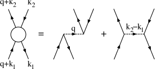
Figure 1: Direct and Exchange parts of the ph interaction.

For a finite range interaction whose spin-isospin dependence is described by the usual Wigner, Bartlett, Heisenberg and Majorana terms, the components $V_{ph}^{(\alpha)}({\bf q},{\bf k}_{1},{\bf k}_{2})$ are:

$$V_{ph}^{(\alpha)}({\bf q},{\bf k}_{1},{\bf k}_{2}) = D^{(\alpha)}f(q)+E^{(\alpha)}h({\bf k}_{1}-{\bf k}_{2})+R^{(\alpha)}~{}.$$ (2)

The direct terms $D^{(\alpha)}f(q)$ depend only on the modulus $q$ while the exchange terms $E^{(\alpha)}h({\bf k}_{1}-{\bf k}_{2})$ depend on ${\bf k}_{1}-{\bf k}_{2}$. The last term $R^{(\alpha)}$ accounts for rearrangement contributions and it must be included if the starting nucleon-nucleon effective interaction has a density dependence rin80 .

As an example, let us consider as the starting interaction $V$ the effective Gogny force gog75 which is often used for nuclear matter and nuclear structure studies. It consists of a sum of two Gaussians having different ranges and spin-isospin dependences supplemented by a contact term depending on the local density. For such a force, the functions $f(q)$ and $h({\bf k}_{1}-{\bf k}_{2})$ are:

$$f(q) = e^{-\frac{1}{4}q^{2}\mu^{2}}$$

$$h({\bf k}_{1}-{\bf k}_{2}) = e^{-\frac{1}{4}({\bf k_{1}}-{\bf k_{2}})^{2}\mu^{2}}~{},$$ (3)

where $\mu$ is the range parameter of the Gaussian form factor. For a Gogny-type force, the direct and exchange contributions to Eq. (2) are obtained by summing over the two Gaussians. The expressions of $D^{(\alpha)}$ and $E^{(\alpha)}$ in terms of the spin-isospin coefficients and the range of the Gaussian, as well as the rearrangement term $R^{(\alpha)}$ are shown in Table 1.

$(S,T)$	(0,0)	(0,1)	(1,0)	(1,1)
$D^{(S,T)}$	$\pi\sqrt{\pi}\mu^{3}(4W+2B-2H-M)$	$\pi\sqrt{\pi}\mu^{3}(-2H-M)$	$\pi\sqrt{\pi}\mu^{3}(2B-M)$	$\pi\sqrt{\pi}\mu^{3}(-M)$
$E^{(S,T)}$	$\pi\sqrt{\pi}\mu^{3}(-W-2B+2H+4M)$	$\pi\sqrt{\pi}\mu^{3}(-W-2B)$	$\pi\sqrt{\pi}\mu^{3}(-W+2H)$	$\pi\sqrt{\pi}\mu^{3}(-W)$
$R^{(S,T)}$	$\frac{3}{2}(\gamma+1)(\gamma+2)t_{3}\rho^{\gamma}$	$-\,(1+2x_{3})t_{3}\rho^{\gamma}$	$-\,(1-2x_{3})t_{3}\rho^{\gamma}$	$-\,t_{3}\rho^{\gamma}$

Table 1: Direct, exchange and density-dependent components of the p-h interaction corresponding to a Gogny-type interaction. $W,B,H,M,\mu,t_{3},\gamma$ are interaction parameters, $\rho$ is the local density.

Let us consider for simplicity an infinite nuclear medium at zero temperature and unpolarized both in spin and isospin spaces. At mean field level this system is described as an ensemble of independent nucleons moving in a self-consistent mean field generated by the starting effective interaction treated in the Hartree-Fock (HF) approximation. The momentum dependent HF mean field, or self-energy determines the single-particle spectrum $\epsilon(k)$ and the Fermi level $\epsilon(k_{F})$.

To calculate the response of the medium to an external field it is convenient to introduce the p-h Green’s function, or retarded p-h propagator $G({\bf q},\omega,{\bf k}_{1})$. From now on we choose the $z$ axis along the direction of ${\bf q}$. In the HF approximation, the p-h Green’s function is the free retarded p-h propagator walecka :

$$G^{(0)}(q,\omega,{\bf k}_{1})=\frac{\theta(k_{F}-k_{1})-\theta(k_{F}-|{\bf q}+{\bf k_{1}}|)}{\omega+\epsilon(k_{1})-\epsilon(|{\bf q}+{\bf k}_{1})|+i\eta}~{}.$$ (4)

It is customary to go beyond the HF mean field approximation and to take into account the long-range type of correlations by resumming a class of p-h diagrams. One thus obtains the well-known Random Phase Approximation (RPA) walecka whose correlated Green’s function $G(q,\omega,{\bf k}_{1})$ satisfies the Bethe-Salpeter equation:

$$G(q,\omega,{\bf k}_{1})=G^{(0)}(q,\omega,{\bf k}_{1})+G^{(0)}(q,\omega,{\bf k}_{1})\,\int\frac{{\rm d}^{3}k_{2}}{(2\pi)^{3}}V_{ph}(q,{\bf k}_{1},{\bf k}_{2})G(q,\omega,{\bf k}_{2})~{}.$$ (5)

Finally, the response function $\chi(q,\omega)$ in the infinite medium is related to the p-h Green’s function by:

$$\chi(q,\omega)=g\int\frac{{\rm d}^{3}k_{1}}{(2\pi)^{3}}G(q,\omega,{\bf k}_{1})~{},$$ (6)

Equations (4- 6) should be understood for each $(S,T)$ channel. The Lindhard function $\chi^{(0)}$ is obtained when the free p-h propagator $G^{(0)}$ is used in Eq. (6).

If the p-h interaction Eq. (2) is treated in some approximation so as to simplify its $\bf{k}_{1}-\bf{k}_{2}$ dependence, then solving Eq. (5) can be made easier. For instance, neglecting the exchange terms $E^{(\alpha)}$, or treating them in Landau approximation and keeping only $l=0$ terms lead to the familiar ring approximation of RPA, and the response function (6) can be expressed in terms of the Lindhard function $\chi^{(0)}$. In the past there have been studies of nuclear matter response functions with Gogny-type interactions under simplifying assumptions. For instance, RPA response functions in the long-wavelength limit, i.e., for vanishing momentum transfer $q$ have been calculated in Ref. gog77 . Actually, that study was done in the Landau approximation whereas we are looking for a complete RPA calculation with finite range interactions.

The method presented in this paper allows one to obtain RPA Green’s functions for all values of $q$ and $\omega$ without further approximation. This will be useful for studying processes such as the propagation of particles inside nuclear matter. It is a cumbersome task to solve directly in the 3-dimensional momentum space the Bethe-Salpeter equation with the full p-h residual interaction. The general method of solution proposed here is to expand the Green’s functions and the p-h interaction on a complete basis of spherical harmonics and to transform Eq. (5) into a set of coupled integral equations on the radial momentum (i.e., the momentum modulus) variable. The expansion of the unperturbed p-h Green’s function is simple because it has no dependence on the angle $\phi$ of the vector ${\bf k}_{1}$:

$$G^{(0)}(q,\omega,{\bf k}_{1})=\sum_{L}G_{L}^{(0)}(q,\omega,k_{1})Y_{L0}(\hat{k}_{1})~{}.$$ (7)

As for the residual interaction Eq. (2) it depends on the modulus $|\bf{k}_{1}-\bf{k}_{2}|$ and therefore, its expansion is:

$$V_{ph}(q,{\bf k}_{1},{\bf k}_{2})=\sum_{LM}V_{L}(q,k_{1},k_{2})Y_{LM}^{*}(\hat{k}_{1})Y_{LM}(\hat{k}_{2})~{}.$$ (8)

Because of the structure of the multipole expansion of $V_{ph}$, the expansion of the RPA Green’s function is similar to that of $G^{(0)}$:

$$G(q,\omega,{\bf k}_{1})=\sum_{L}G_{L}(q,\omega,k_{1})Y_{L0}(\hat{k}_{1})~{}.$$ (9)

Indeed, by inserting back this expansion of the propagator into Eq. (5), a consistent result is obtained. Making use of the multipole expansions (7-9) one can transform the Bethe-Salpeter equation into a set of coupled integral equations for the multipole components of the RPA Green’s function:

$$G_{L}(q,\omega,k_{1})=G^{(0)}_{L}(q,\omega,k_{1})+\sum_{L^{\prime}}\int\frac{k_{2}^{2}dk_{2}}{(2\pi)^{3}}F_{LL^{\prime}}(q,\omega;k_{1},k_{2})G_{L^{\prime}}(q,\omega,k_{2})~{},$$ (10)

where we have defined

$$F_{LL^{\prime}}(q,\omega;k_{1},k_{2})=\Big{(}\sum_{\lambda}\Big{[}\frac{(2L+1)(2L^{\prime}+1)}{4\pi(2\lambda+1)}\Big{]}^{\frac{1}{2}}(L0L^{\prime}0|\lambda 0)^{2}G^{(0)}_{\lambda}(q,\omega,k_{1})\Big{)}V_{L^{\prime}}(q,k_{1},k_{2})~{},$$ (11)

where $(L_{1}M_{1}L_{2}M_{2}|L_{3}M_{3})$ is a Clebsh-Gordan coefficient. The angular momenta $L$ and $L^{\prime}$ entering the above expressions are unlimited in principle. We will see in the next section that in practice the convergence is very fast and very few terms are necessary to obtain a good accuracy. Finally, the response function Eq. (6) can be expressed as:

$$\chi(q,\omega)=\frac{\sqrt{4\pi}}{(2\pi)^{3}}g\int G_{L=0}(q,\omega,k)k^{2}dk~{},$$ (12)

where only the $L=0$ multipole of the RPA Green’s function is required. However, one has to solve the full system of coupled equations (10), since the interaction couples different multipoles. In practice, a complete calculation implies the choice of a cut-off value $L_{max}$ for the summations on angular momenta, and a grid of points in momentum space in order to transform the integrals into discrete sums. Then, Eq. (10) is solved by a matrix inversion. For the results presented in the next sections we have chosen a grid with a constant number of points. With 100 points, we have obtained a good comparison of the free response function with its analytic form, the Lindhard function. The upper limit is $k_{max}=k_{F}+q$. Hence, for $q=k_{F}/10$, $\Delta k$=0.017 fm^-1 and $k_{max}$=1.71 fm^-1 and for $q=k_{F}$, $\Delta k$=0.031 fm^-1 and $k_{max}$=3.14 fm^-1.

III Symmetric nuclear matter results

The Gogny force D1S gog75 has been chosen to discuss some results calculated in symmetric nuclear matter. First, the unperturbed p-h Green’s function $G^{(0)}(q,\omega,{\bf k})$ is calculated using the Hartree-Fock solution corresponding to D1S. It is just the familiar Lindhard function and the multipoles $G^{(0)}_{L}(q,\omega,k)$ can be easily calculated numerically. Then, an important practical issue is the sensitivity of the solution of Eq. (10) to the number of multipoles included in the calculation. To examine this point we have performed calculations with different values of $L_{max}$. In Figs. 2-3 the real and imaginary parts of the RPA response function $\chi^{(0,0)}(q,\omega)$ are displayed for several values of $L_{max}$ and two values of $q$, namely 27 MeV ($\simeq k_{F}/10$) and 270 MeV ($\simeq k_{F}$).

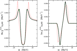
Figure 2: Real and imaginary parts of the response function $\chi^{(0,0)}$ for $q$=27 MeV. Dotted: $L_{max}=0$. Dashed: $L_{max}=1$. Solid: $L_{max}=2$ (converged).

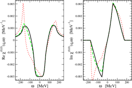
Figure 3: Same as Fig.1 for $q$=270 MeV.

It can be seen that for small $q$ the convergence is reached for $L_{max}$=1 (the solid and dashed curves are indistinguishable in the figure). Increasing the value of $q$, one sees that there is still a small difference between $L_{max}$=1 and 2. The convergence is reached in fact for $L_{max}$=3.

A quantitative measure of the degree of convergence can be provided by the expected symmetries of the real and imaginary parts of the response functions. Indeed, the former should be symmetric and the latter anti-symmetric with respect to $\omega$=0. Let us introduce for this purpose the following symmetry parameters:

$$s_{r} = \int_{\omega\geq 0}{\rm d}\omega\,|{\rm Re}\chi(\omega)-{\rm Re}\chi(-\omega)|\bigg{/}\int_{\omega\geq 0}{\rm d}\omega\,|{\rm Re}\chi(\omega)+{\rm Re}\chi(-\omega)|~{},$$

$$s_{i} = \int_{\omega\geq 0}{\rm d}\omega\,|{\rm Im}\chi(\omega)+{\rm Im}\chi(-\omega)|\bigg{/}\int_{\omega\geq 0}{\rm d}\omega\,|{\rm Im}\chi(\omega)-{\rm Im}\chi(-\omega)|~{}.$$ (13)

The results corresponding to the cases shown in Figs. (2-3) are indicated in Table 2. Although the mentioned symmetric behavior is seen in the figures, the results of Table 2 allow one to conclude more quantitatively that, in the range of momentum transfer up to $k_{F}$, the symmetry criteria are satisfied within 1% using $L_{max}$=3. In this case, the matrices involved in the solution of Eq. (10) have relatively moderate sizes (less than 500x500) and the calculations are rather fast. A similar numerical study for the response functions in the channels other than ($S=0,T=0$) has been performed, leading to the same type of convergence as a function of $L_{max}$.

		$L_{max}$
	$q$ (MeV)	0	1	2	3	4	5
$10^{2}s_{r}$	27	2.10	2.27	0.42	0.06	-	-
	270	14.7	14.0	3.75	0.94	0.56	0.52
$10^{2}s_{i}$	27	3.60	2.32	0.60	0.12	-	-
	270	14.0	13.0	3.38	0.85	0.36	0.35

Table 2: Symmetry parameters corresponding to the cases shown in Figs. 2-3.

To understand this rapid convergence, it is necessary to analyze in some detail the multipoles of the p-h interaction. To this end, we plot the dimensionless multipoles

$$\tilde{V}_{L}(q,k_{1},k_{2})\equiv\frac{2L+1}{4\pi g}N_{0}V_{L}(q,k_{1},k_{2})$$ (14)

for a fixed value of $q$ in the plane ($k_{1}/k_{F}$,$k_{2}/k_{F}$) of hole momenta. In this expression, $N_{0}=gm^{*}k_{F}/(2\pi^{2})$ is the density of states, and the factor multiplying $V_{L}$ fixes the scale: the value at $q$=0, $k_{1}=k_{2}=k_{F}$ gives the familiar Landau dimensionless parameter. The factor $4\pi$ comes from the use of spherical harmonics $Y_{L0}$ instead of Legendre polynomials $P_{L}$ in the multipole expansions.

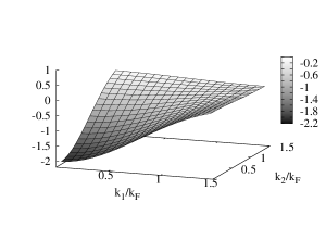
Figure 4: The dimensionless monopole $\tilde{V}_{0}^{(0,0)}(q,k_{1},k_{2})$ as a function of the momenta $k_{1}/k_{F}$ and $k_{2}/k_{F}$ at $\rho=\rho_{0}$. The left panel represents the case $q$=0 and the right one $q$=270 MeV.

The monopole $L$=0 case is plotted in Fig. 4 for $q$=0 (left panel) and $q$=270 MeV (right panel). The effect of a finite transferred momentum $q$ only affects the monopole component of the p-h interaction (see Eq. 2), and it produces an overall translation of the interactions drawn in the figure. For this specific channel, it induces a repulsion.

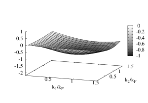
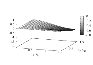
Figure 5: The dimensionless multipoles $\tilde{V}_{L}^{(0,0)}(q,k_{1},k_{2})$ as a function of the momenta $k_{1}/k_{F}$ and $k_{2}/k_{F}$ at $\rho=\rho_{0}$. The left panel represents the case $L$=1 and the right one $L$=2.

The multipoles $L$=1 and $L$=2 are plotted in Fig. 5, in the left and right panels respectively. This series of figures for $L$=0,1,2 shows explicitly that the multipole expansion of the p-h interaction is rapidly converging after the first few angular momenta.

Inside the ($k_{1}$,$k_{2}$) domain considered, the variations of the multipoles $V_{L}$ span the range of values (-2:1) for $L$=0, (-1:0) for $L$=1, (-0.5:0) for $L$=2, (-0.3:0) for $L$=3 while beyond $L$=4, the multipoles are practically negligible. In conclusion, the full convergence is achieved using $L_{max}$=3.

IV Landau approximations

Once the convergence of the method has been proved, it is useful to analyze some approximations employed to obtain the response function. The Landau-Migdal approximation migdal is often used in the literature because it simplifies greatly the calculation of RPA response functions. This approximation was used in Ref. gog77 for the Gogny interaction D1, based on the solution of the kinetic equations. We should mention that no analysis of convergence was made. The approximation consists in assuming that the interacting particle and hole are on the Fermi surface and that the interaction takes place only in the limit $q=0$. That is to say that each multipole of the p-h interaction is replaced by the constant $V_{L}(0,k_{F},k_{F})$. The validity of this assumption can be checked by inspecting Figs. 4-5. For the considered interaction and $(S,T)$ channel, the first Landau dimensionless parameters are $F_{0}$=-0.38, $F_{1}$=-0.91 and $F_{2}$=-0.33. It can be seen in these figures that the corresponding multipoles of the p-h interaction are far from taking a constant value. It is well known that the validity of the approximation is limited to very small values of $q$, because in this case the physically relevant values of $k_{1}$ and $k_{2}$ remain around the Fermi momentum. However, it is worth keeping in mind that in what concerns the response function the differences between the true and the approximated p-h interactions are smeared out by the kinetic constraints of the phase space.

The $q$=0 hypothesis can be easily relaxed. Indeed, Eq. (2) shows that only the exchange of the p-h interaction depends on $k_{1}$ and $k_{2}$. Thus, we could keep unchanged the direct term $D^{(\alpha)}f(q)$ of the interaction Eq. (6) with its full $q$-dependence and make the Landau approximation on the exchange term $E^{(\alpha)}h({\bf k}_{1}-{\bf k}_{2})$ only. We denote this choice as the Landau Approximation For Exchange Term (LAFET). One may hope that this procedure will improve the usual Landau approximation by treating approximately the exchange term only. The simplicity of the Landau approximation is preserved, the only change being that the monopole contribution acquires a $q$-dependence coming from the direct term.

The general method presented in Sec. II can be easily applied to both approximations. In the appendix A, it is shown that if the p-h interaction is independent of the hole momenta $k_{1}$ and $k_{2}$, the system of coupled integral equations Eq. (10) for the multipoles $G_{L}(q,\omega,k)$ can be transformed into a set of algebraic equations for their integrals $\int dkk^{2}G_{L}(q,\omega,k)$.

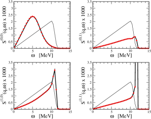
Figure 6: Structure function $S^{(S,T)}(q,\omega)$ for $q$=27 MeV and $L_{max}=3$. Solid thin curve: HF. Dotted: Landau. Dashed: LAFET. Solid thick line: converged.

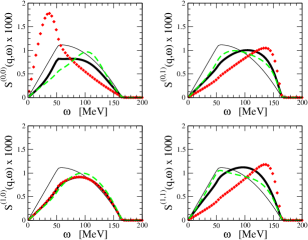
Figure 7: Structure function $S^{(S,T)}(q,\omega)$ for $q$=270 MeV and $L_{max}=3$. Solid thin curve: HF. Dotted: Landau. Dashed: LAFET. Solid thick line: converged.

We represent on Figs. 6-7 a comparison of the structure function

$$S^{(S,T)}(q,\omega)=-\frac{1}{\pi}{\rm Im}\chi^{(S,T)}(q,\omega)$$ (15)

extracted from a converged solution (solid thick curve) with Landau (dotted) and LAFET (dashed) approximations for $q=k_{F}/10$ and $q=k_{F}$. The HF solution (solid thin curve) is also displayed as a reference. All the curves shown correspond to $L_{max}$=3, to guarantee the convergence of the solution as shown in Sec. III. As expected, the Landau approximation is a good one for small transferred momentum $q$ and all $(S,T)$ channels. However, for the highest transferred momentum considered in this paper, the validity of the Landau approximation and LAFET response functions is very $(S,T)$ dependent. As a rule, LAFET induces a response closer to the exact one. Hence, LAFET could be considered as a very simple extension of the Landau approximation which allows one to evaluate processes which involve finite transferred momenta.

There are situations where it is necessary to calculate accurately response functions of a nuclear medium to an external probe, as we already mentioned in the introduction. When the transferred momenta are not small compared to the Fermi momentum, one must perform the full calculations with the method presented in Sec. II. Alternatively, it is possible to use the LAFET method, which is very simple and efficient if extensive calculations are needed, and improves the Landau approximation.

V Conclusion

The main purpose of this work is to present a general method for obtaining nuclear response functions in an infinite medium within a Hartree-Fock-RPA framework. Starting with finite range effective interactions like the Gogny interaction, approximate methods using the Landau approximation are available in the literature, but surprisingly not much beyond this approximation can be found. The method proposed here simply consists in expanding the Bethe-Salpeter equation onto a spherical harmonics basis and therefore, the calculations can be carried out in principle up to any degree of accuracy if one includes a sufficient number of partial waves. In practice, the case study that we have discussed in this work shows that the convergence is very fast and that the number of multipoles needed is very small. This result holds not only for small values of momentum transfer but even at values in the range of the Fermi momentum. The fast convergence is related to the properties of the effective p-h interaction.

This general method of solving the Bethe-Salpeter equation suggests also an approximation scheme beyond the standard Landau approximation, the LAFET scheme where the full $q$-dependence is kept in the direct p-h interaction and the Landau approximation is done only on the exchange p-h interaction. The standard Landau approximation and LAFET are compared with the exact response functions and it is shown that the LAFET results show an improved agreement with the exact results. This approximation can be useful for extensive calculations when the numerical effort required by exact calculations becomes heavy.

Acknowledgments

This work is supported in part by the grant FIS2004-0912 (MEC, Spain) and by the IN2P3(France)-CICYT(Spain) exchange program. We thank P. Schuck for bringing to our attention the work quoted in Ref. gog77 .

Appendix A Landau approximations

Let us show that if the p-h interaction is independent of the hole momenta $\bf{k_{1}}$ and $\bf{k_{2}}$, the system of coupled integral equations Eq. (10) for the multipoles $G_{L}(q,\omega,k)$ can be transformed into a set of algebraic equations for the following quantities

$$R_{L}(q,\omega)=g\frac{\sqrt{4\pi}}{(2\pi)^{3}}\int dkk^{2}G_{L}(q,\omega,k)~{}.$$ (16)

The factors before the integral are chosen such that the response function is given by $R_{L=0}$.

Let us consider the multipoles of the p-h interaction, Eq. (8), in the particular case where the hole momenta $\bf{k_{1}}$ and $\bf{k_{2}}$ lie on the Fermi surface. For this specific interaction, the functions $F_{LL^{\prime}}$ entering Eq. (11) no longer depend on $k_{2}$. Since all the momentum dependence is now contained in the p-h propagators, $G_{L}$ and $G_{L}^{(0)}$, integrating over $k_{1}$ the system Eq. (10) can be transformed into the set of equations:

$$R_{L}(q,\omega)=R_{L}^{(0)}(q,\omega)+\sum_{LL^{\prime}}A_{LL^{\prime}}(q,\omega)R_{L^{\prime}}(q,\omega)~{},$$ (17)

where $R_{L}^{(0)}$ is defined as in Eq. (16) for the free propagator and

$$A_{LL^{\prime}}(q,\omega)=\frac{{\tilde{V}}_{L^{\prime}}(q,k_{F},k_{F})}{N_{0}}\sum_{\lambda}\Big{[}\frac{(2L+1)}{(2L^{\prime}+1)(2\lambda+1)}\Big{]}^{\frac{1}{2}}(L0L^{\prime}0|\lambda 0)^{2}R^{(0)}_{\lambda}(q,\omega)~{}.$$ (18)

It is worth noting that the Landau parameters are given by $f_{L}\equiv{\tilde{V}}_{L}(q=0,k_{F},k_{F})/N_{0}$.

As an example, we give here the response function in the Landau approximation with $L_{max}$=2:

$$\chi=\frac{\chi^{(0)}}{1-W\chi^{(0)}}~{},$$ (19)

where

$$W=f_{0}-\frac{1}{2}f_{2}+\nu^{2}\frac{f_{1}+(\frac{27}{8}\nu^{2}+\frac{3}{10}F_{1})f_{2}}{\left(1+\frac{1}{3}F_{1}\right)\left(1+\frac{1}{8}[-9\nu^{2}+\frac{12}{5}]F_{2}\right)}$$ (20)

plays the role of the induced p-h interaction. In this expression, we have defined $\nu=\omega m^{*}/(qk_{F})$, and $F_{i}=f_{i}N_{0}$ are the dimensionless Landau parameters.

References

- (1) R.B. Wiringa, Revs. Mod. Phys. 65, 231 (1993).
- (2) A. Akmal, V.R. Pandharipande, D.G. Ravenhall, Phys. Rev. C 58, 1804 (1998).
- (3) W. Zuo, A. Lejeune, U. Lombardo, J.-F. Mathiot, Nucl. Phys. A 706, 418 (2002).
- (4) R. Brockmann, R. Machleidt, Phys. Lett. B 149, 28 3 (1984).
- (5) B. ter Haar, R. Malfliet, Phys. Rep. 149, 207 (1987).
- (6) D. Vautherin, D.M. Brink, Phys. Rev. C5, 626 (1972).
- (7) E. Chabanat, P. Bonche, P. Haensel, J. Meyer, R. Schaeffer, Nucl. Phys. A 627, 710 (1997) .
- (8) D. Gogny, Proc. Int. Conf. Nuclear Self-consistent Fields, G. Ripka and M. Porneuf eds., North-Holland, Amsterdam (1975).
- (9) C. Garcia-Recio, J. Navarro, N. Van Giai, L.L. Salcedo, Ann. Phys. 214, 293 (1992).
- (10) D. Gogny, R. Padjen, Nucl. Phys. A 293, 365 (1977).
- (11) P. Ring and P. Schuck, The nuclear many-body problem, (Springer, 1980).
- (12) A.L. Fetter and J.D. Walecka, Quantum Theory of Many-Particle Systems, McGraw-Hill (New York, 1971).
- (13) A.B. Migdal, Theory of Finite Fermi Systems and Applications in Atomic Nuclei (Wiley, New York, 1967).