Wavelet Methods in the Relativistic Three-Body Problem

Abstract

Abstract: In this paper we discuss the use of wavelet bases to solve the relativistic three-body problem. Wavelet bases can be used to transform momentum-space scattering integral equations into an approximate system of linear equations with a sparse matrix. This has the potential to reduce the size of realistic three-body calculations with minimal loss of accuracy. The wavelet method leads to a clean, interaction independent treatment of the scattering singularities which does not require any subtractions.

I Introduction

This is the third paper kessler03 kessler04 in a series of investigations designed to explore potential advantages of using wavelet numerical analysis to solve the relativistic three-body problem. Commercially, wavelets are used to convert raw digitized photographic images to compressed JPEG files jpeg . In this application the data compression leads to a large saving in storage space with a minimal loss of information. The compression involves expanding the raw digital image in a wavelet basis and setting the smaller expansion coefficients to zero. The kernel of a scattering integral equation and a raw digital image can both be approximated by rectangular arrays of numbers with some continuity properties. This suggests that the bases used to compress digital images could be used to generate accurate sparse matrix approximations to the kernel.

The ability to construct numerically exact solutions to the quantum mechanical three-body problem coupled with the ability to accurately measure complete sets of experimental observables constrains the form of the three-nucleon Hamiltonian. These constraints have resulted in the construction of realistic model nucleon-nucleon interactions deSwart v18 cdbonn . When these interactions are used in the many-nucleon Hamiltonian, the resulting dynamical model provides a good quantitative description of low-energy nuclear physics lightnuc .

The state of the art in few-body computations has improved to the point where numerically exact scattering calculations at energy and momentum transfers of hundreds of $MeV$ have been performed walter . Higher energy calculations are possible. As in the low-energy case, the structure of Hamiltonians for higher energy reactions can be constrained by the consistency of the few-body calculations with precise measurements of complete sets of experimental observables.

The success of the few-body approach to low-energy nuclear physics is a consequence of (1) knowing the relevant degrees of freedom (nucleons), (2) working with the most general Hamiltonians involving these degrees of freedom that are consistent with the symmetries of the system (Galilean invariance) and (3) understanding the relation between the few and many-body problem (cluster properties). To extend this success to reactions involving higher energy scales (1) the relevant degrees of freedom may have to include explicit mesonic or sub-nucleonic degrees of freedom (2) Galilean invariance must be replaced by Poincaré invariance and (3) cluster properties must be maintained.

Each of the required extensions of low-energy nuclear dynamics is non-trivial, and progress has been made on all three problems walter wp91 wp02 fuda wp03 . The purpose of this paper is to focus on technical aspects of using wavelet numerical analysis to construct exact numerical solutions of the dynamics in Poincaré invariant few-body models. While the scope of this paper is limited to three-nucleon models with no explicit mesonic or subnucleonic degrees of freedom and S-matrix cluster properties fritz65 , the formulation and advantage of methods discussed in this paper are straightforward to extend to systems with explicit mesonic degrees of freedom and stronger forms of cluster properties wp03 . Moving singularities are a generic feature of the dynamical equations in all of these cases.

Relativistic few-body equations are naturally formulated in momentum space. Relativistic kinematic factors, Wigner rotations and Melosh rotations are all multiplication operators in momentum space. The compactness of the iterated Faddeev-Lovelace kernel implies the kernel of the integral equations can be uniformly approximated by a finite matrix, resulting in a finite linear system. In the momentum representation these linear systems have large dense matrices, which increase in size with increasing energy and momentum transfer. It is desirable to be able to perform accurate calculations at energy and momentum scales where subnuclear degrees of freedom are relevant. At these scales a relativistic treatment is required and advances in computational efficiency are needed to perform realistic calculations. The ability of the wavelet transform to efficiently transform a dense matrix to an approximate sparse matrix suggests that wavelet methods can provide a powerful tool for improving the efficiency of relativistic few-body computations.

The advantages of using wavelet numerical analysis to solve momentum space scattering integral equations was investigated in kessler03 and kessler04 . These papers used wavelet numerical analysis to solve the Lippmann-Schwinger equation for a system of two nucleons interacting with a Malfliet Tjon V potential Tjon Payne using partial wave expansions kessler03 and direct integration kessler04 . In both applications the kernel of the integral equation was accurately approximated by a sparse matrix, which resulted in accurate approximate solutions. The success of these applications indicates that wavelet numerical analysis will have similar advantages when applied to the relativistic three-body problem.

The feature of the three-body problem that is not present in the two-body applications is moving singularities. The methods used in kessler03 and kessler04 are not applicable to problems with moving singularities. The purpose of this paper is to illustrate how to apply wavelet numerical analysis to treat the moving singularities that appear in the relativistic three-body problem.

II Overview - Wavelet Numerical Analysis

The applications in ref. kessler03 and kessler04 used Daubechies’ wavelets. These wavelets differ from the wavelets used to store JPEG images. The Daubechies’ wavelets are orthonormal but the basis functions are not reflection symmetric; while the wavelets used to store JPEG images sacrifice orthonormality to obtain more symmetric basis functions. The results of ref. kessler03 and kessler04 indicate that the Daubechies’ wavelets are suitable for scattering calculations.

Daubechies’ wavelets Daubechies Daubechies2 are discussed in many texts on wavelets Kaiser Resnik Strang jorgensen . They are fractal functions that have complex structures on all scales. Because the basis functions have structure on all scales, numerical applications with wavelets require a different approach to numerical analysis, hence the term wavelet numerical analysis.

We use the Daubechies’ wavelets because they are a dense orthonormal set of compactly supported functions with the property that finite linear combinations can locally pointwise represent low-degree polynomials.

Two types of functions are needed to generate wavelet bases. These functions are called scaling functions and wavelets. The scaling function, $\phi(x)$, is the solution of the linear renormalization group equation:

$$D\phi(x)=\sum_{l=0}^{2K-1}h_{l}T^{l}\phi(x)$$ (1)

with normalization

$$\int_{-\infty}^{\infty}\phi(x)dx=1.$$ (2)

Equation (1) is called the scaling equation.

In equation (1) $D$ is the unitary scaling operator

$$Df(x):={1\over\sqrt{2}}f({x\over 2})$$ (3)

which stretches the support of the function by a factor of two. The operator $T$ is the unitary unit translation operator

$$Tf(x)=f(x-1).$$ (4)

The coefficients $h_{l}$ are real numbers that determine the properties of the scaling function. $K$ is a finite positive integer. The calculations in kessler03 kessler04 used Daubechies’ $K=3$ wavelets. The reason for this choice will be discussed later. For the $K=3$ Daubechies’ wavelets the six scaling coefficients $h_{l}$ are given in Table 1.

Table 1: Daubechies’ $K=3$ Scaling Coefficients
$h_{l}$ K=3 $h_{0}$ $(1+\sqrt{10}+\sqrt{5+2\sqrt{10}})/16\sqrt{2}$ $h_{1}$ $(5+\sqrt{10}+3\sqrt{5+2\sqrt{10}})/16\sqrt{2}$ $h_{2}$ $(10-2\sqrt{10}+2\sqrt{5+2\sqrt{10}})/16\sqrt{2}$ $h_{3}$ $(10-2\sqrt{10}-2\sqrt{5+2\sqrt{10}})/16\sqrt{2}$ $h_{4}$ $(5+\sqrt{10}-3\sqrt{5+2\sqrt{10}})/16\sqrt{2}$ $h_{5}$ $(1+\sqrt{10}-\sqrt{5+2\sqrt{10}})/16\sqrt{2}$

The fractal structure of $\phi(x)$ is a consequence of the scaling equation (1) which shows that the scaling function on a given scale is a finite linear combination of translates of the same function on half the scale.

The scaling equation implies that the scaling coefficients $h_{l}$ satisfy

$$\sum_{l=0}^{2K-1}h_{l}=\sqrt{2}$$ (5)

and that the solution $\phi(x)$ of equation (1) has support on the interval $[0,2K-1]$ waverev .

The unit translates of the scaling function are orthonormal

$$(T^{m}\phi,T^{n}\phi)=\delta_{mn}$$ (6)

provided the scaling coefficients satisfy the additional constraints:

$$\sum_{l=0}^{2K-1}h_{l}h_{l-2m}=\delta_{m0}.$$ (7)

The scaling function $\phi(x)$ is continuous (for $K>1$) and can be computed exactly at all dyadic rationals using equations (1) and (2). This method is used to compute the Daubechies’ $K=3$ scaling function plotted in Figure 1.

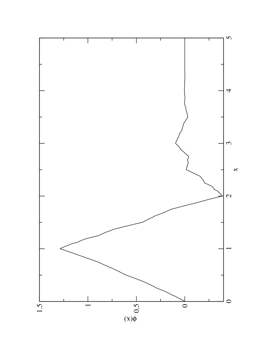
Figure 1: Daubechies’ $K=3$ scaling function.

The subspace of square integrable functions on the real line that can be expressed as linear combinations integer translates of the scaling function, $T^{n}\phi(x)$, is the subspace ${\cal V}_{0}$ of $L^{2}({\mathbb{R}})$ defined by :

$${\cal V}_{0}:=\{f(x)=\sum_{n=-\infty}^{\infty}f_{n}T^{n}\phi(x)|\sum_{n=-\infty}^{\infty}|f_{n}|^{2}<\infty\}.$$ (8)

Application of powers of the scaling operator $D^{k}$ to ${\cal V}_{0}$ defines subspaces ${\cal V}_{k}$ with coarser $(k>0)$ or finer resolution $(k<0)$:

$${\cal V}_{k}=D^{k}{\cal V}_{0}.$$ (9)

The space ${\cal V}_{k}$ is called the approximation space with resolution $k$. The resolution determines the size of the smallest features that can be approximated by functions in ${\cal V}_{k}$.

The scaling functions

$$\phi_{kn}(x):=D^{k}T^{n}\phi(x)={1\over 2^{k/2}}\phi({x\over 2^{k}}-n)$$ (10)

are an orthonormal basis for ${\cal V}_{k}$. The support of $\phi_{kn}(x)$ is $[2^{k}n,2^{k}(n+2K-1)]$.

The scaling equation implies the inclusions

$${\cal V}_{k}\supset{\cal V}_{k+1}.$$ (11)

The orthogonal compliment of ${\cal V}_{k+1}$ in ${\cal V}_{k}$ is denoted by ${\cal W}_{k+1}$ which leads to the orthogonal decomposition

$${\cal V}_{k}={\cal V}_{k+1}\oplus{\cal W}_{k+1}.$$ (12)

Orthonormal basis functions, $\psi_{km}(x)$, for the subspaces ${\cal W}_{k}$ are elements of ${\cal V}_{k-1}$ given by

$$\psi_{km}(x)=D^{k}T^{m}\psi(x)$$ (13)

$$\psi(x)=\sum_{l=0}^{2K-1}g_{l}D^{-1}T^{l}\phi(x)$$ (14)

where

$$g_{l}=(-)^{l}h_{2K-1-l}.$$ (15)

The subspaces ${\cal W}_{kn}$ are called the wavelet spaces and the basis functions $\psi_{kn}$ are called wavelets. The support of $\psi_{kn}(x)$ is identical to the support of $\phi_{kn}(x)$. Since the wavelets are finite linear combinations scaling functions they are also fractal functions.

The function $\psi(x)=\psi_{00}(x)$ is called the mother wavelet; the Daubechies’ $K=3$ mother wavelet is shown in Figure 2.

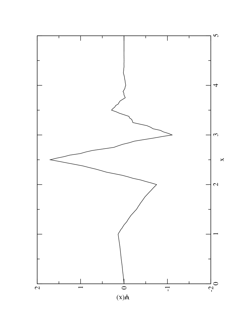
Figure 2: Daubechies’ $K=3$ mother wavelet.

The coefficients $h_{l}$ for the Daubechies’ $K$ wavelets are determined by equations (5) and (7) and the requirements

$$\int_{-\infty}^{\infty}\psi(x)x^{n}dx=0;\qquad n=0,1,\cdots,K-1$$ (16)

which implies that $\psi_{km}(x)$ is locally orthogonal to all polynomials of degree $K-1$. Equation (16) can be expressed directly in terms of the scaling coefficients:

$$\sum_{l=0}^{2K-1}l^{k}g_{l}=$$

$$\sum_{l=0}^{2K-1}l^{k}(-)^{l}h_{2K-1-l}=0\qquad k=0\cdots K-1.$$ (17)

For any $K>0$ conditions (5), (7) and (17) determine $h_{l}$ up to reflection,

$$h_{l}\to h^{\prime}_{l}:=h_{2K-1-l}.$$ (18)

The entries in Table 1 are the solution of these equations for $K=3$. The Daubechies’ wavelets have the property that as $k\to-\infty$ (infinitely fine resolution) the space ${\cal V}_{k}$ becomes all of $L^{2}(\mathbb{R})$.

The decomposition (12) implies that

$${\cal V}_{k}={\cal W}_{k+1}\oplus{\cal W}_{k+2}\cdots{\cal W}_{k+m-1}\oplus{\cal W}_{k+m}\oplus{\cal V}_{k+m},$$ (19)

for any $m>0$. This means that functions in the approximation space ${\cal V}_{k}$ can be expanded as linear combinations of the scaling basis functions of resolution $k$ or equivalently as linear combinations of the scaling basis functions of a coarser resolution $k^{\prime}=k+m$ and wavelet basis functions of all resolutions from $k+1$ to $k+m$.

If we let $k\to-\infty$ with $m+k$ finite, then the functions in (19) become a basis for $L^{2}({\mathbb{R}})$. Since the $\psi_{kn}(x)$ basis functions are locally orthogonal to degree $K-1$ polynomials, and only a finite number of the $\phi_{kn}(x)$ are non-zero at any $x$, it follows that finite linear combinations of $\phi_{k,n}(x)$ must be able to locally pointwise represent degree $K-1$ polynomials.

Thus, for the Daubechies’ $K=3$-wavelets finite linear combinations of the scaling basis functions $\phi_{kn}(x)$ can locally pointwise represent polynomials of degree 2, while the wavelet basis functions $\psi_{kn}(x)$ are orthogonal to degree 2 polynomials.

Equation (19) implies that the projection $P_{k}$ of a function $f(x)$ on ${\cal V}_{k}$ can be represented by

$$P_{k}f(x)=\sum_{n}a_{n}\phi_{kn}(x)\qquad a_{n}=\int f(x)\phi_{kn}(x)dx$$ (20)

or equivalently

$$P_{k}f(x)=\sum_{n}a_{n}\phi_{k+m,n}(x)+\sum_{k^{\prime}=k+1}^{k+m}b_{k^{\prime}n}\psi_{k^{\prime},n},$$ (21)

$$b_{kn}=\int f(x)\psi_{k,n}(x)dx.$$ (22)

For a sufficiently fine resolution (large $-k$) the scaling basis functions have small support and integrate to a constant. If $f(x)$ varies slowly on intervals of width $(2K-1)2^{k}$ then expansion coefficients $a_{n}$ are well approximated by evaluating $f(x)$ at any point in the support of $\phi_{kn}(x)$ and multiplying by $2^{k/2}$, which is the integral of $\phi_{kn}(x)$. This means that the scaling function basis coefficients, $a_{n}$, are well approximated, up to a fixed multiplicative constant, by sampling the original function. These coefficients play the role of the raw image in a digital photograph. They provide an accurate, but inefficient approximation of the function $f(x)$.

In the representation (21), if $f(x)$ can be accurately approximated by a polynomial of degree $K-1$ on the support of $\psi_{kn}(x)$ then $b_{kn}\approx 0$. This means that if $f(x)$ can be well approximated by low-degree local polynomials with compact support on multiple scales, most of the coefficients $b_{kn}$ will be be small and the function can be accurately approximated by replacing these small coefficients by zero. The mean square error is the sum of the squares of the discarded coefficients, which can be controlled by selecting a maximum size of the discarded coefficients. Even though most of the basis functions in the representation (21) are orthogonal to low degree polynomials, the equivalence between the representations (20) and (21) means that the representation (21) can still locally pointwise represent low degree polynomials. The orthogonal transformation connecting equivalent representations (20) and (21) of ${\cal V}_{k}$ is called the wavelet transform numrec . For $N$ basis functions it can be implemented in $O(N)$ steps, which for large $N$ requires less steps than a fast Fourier transform.

The scaling equation and normalization condition can be used to derive exact expressions for the moments and partial moments of the scaling function

$$\langle x_{kn}^{m}\rangle:=\int\phi_{kn}(x)x^{m}dx$$ (23)

$$\langle x_{kn}^{m}:=\rangle_{[l,l^{\prime}]}\int_{2^{k}l}^{2^{k}l^{\prime}}\phi_{kn}(x)x^{m}\qquad n\leq l,l^{\prime}\leq 2K-1+n$$ (24)

in terms of the scaling coefficients $h_{l}$. Explicit expressions for the moments and partial moments appear in kessler03 , kessler04 , waverev .

For the Daubechies’ $K$ wavelets with $K>1$ the second moment of the scaling function is the square of the first moment. This means that for $K=3$ the first moment provides a single quadrature point that will integrate the scaling function times any second degree polynomial exactly:

$$\int\phi(x)(a+bx+cx^{2})dx=a+b\langle x\rangle+c\langle x\rangle^{2}.$$ (25)

This is called the one-point quadrature. Translating and rescaling leads to one-point quadratures for all of the scaling basis functions $\phi_{kn}(x)$. The choice of $K=3$ Daubechies’ wavelets in kessler03 and kessler04 is motivated by their ability to locally pointwise represent second degree polynomials and to exactly integrate these local polynomials with a one-point quadrature.

In kessler03 , kessler04 and waverev the moments and the scaling equation are used to compute the singular integrals

$$L_{kn}^{\pm}:=\int dx{\phi_{kn}(x)\over x\pm i\epsilon}$$ (26)

to any pre-determined precision.

In applications the integral equation is approximated by projecting on an approximation space ${\cal V}_{k}$ with a finest resolution $k$ dictated by the problem. This projection can be computed efficiently in the scaling basis (20) using the one-point quadrature (25) and the explicit integrals (26). The resulting matrix equation is transformed using the wavelet transform to an equivalent system in the wavelet basis (21). In the transformed basis the kernel of the integral equation decomposes into the sum of a sparse matrix and a small matrix. The kernel is approximated by setting matrix elements of the kernel that are smaller than a threshold value to zero. This results in a sparse matrix approximation. The resulting linear system is solved using sparse matrix iterative techniques, such as the complex biconjugate gradient method numrec golub used in kessler04 . This solution is transformed back to the scaling function representation, using the inverse wavelet transform, and the resulting solution is inserted back in the integral equation to construct an interpolated solution Sloan .

The only wavelet information used in this application is the wavelet transform and moments of the scaling function. These can both be expressed directly in terms of the scaling coefficients $h_{l}$ in Table 1. This means that the basis functions never have to be computed.

The work in references kessler03 kessler04 shows that all of these steps work as expected. These references also discuss technical issues that arise due to the treatment of endpoints when the equations are transformed to a finite interval.

III Dynamical Equations

The general structure of the Faddeev-Lovelace fritz65 wp91 equation in a relativistic quantum theory with three particles of mass $m$ is

$$X(p,q;p^{\prime},q^{\prime})=D(p,q;p^{\prime},q^{\prime})+$$

$$\int_{0}^{\infty}{K(p,q;p^{\prime\prime},q^{\prime\prime},z)dp^{\prime\prime}dq^{\prime\prime}\over z-e_{1}(p^{\prime\prime},q^{\prime\prime})-e_{2}(q^{\prime\prime})}X(p^{\prime\prime},q^{\prime\prime};p^{\prime},q^{\prime})$$ (27)

where

$$e_{1}(p,q)=\sqrt{4p^{2}+4m^{2}+q^{2}}\qquad e_{2}(q)=\sqrt{m^{2}+q^{2}}$$ (28)

and $X=X_{mn}$, $K=K_{mn}$ and $D=D_{mn}$ are complex matrix valued functions. The quantity $K(p,q;p^{\prime},q^{\prime},z)$ is the smooth part of the kernel.

In order to use wavelet methods it is advantageous to transform this equation to a form where functions of the momentum, rather than the energy, are additive in the denominator. This transformation facilitates the treatment of the moving singularity. Note that $e_{1}>e_{2}$ for all values of $p$ and $q$. If $E>0$ then $E+e_{1}(p,q)-e_{2}(q)>0$. It follows that the singular denominator

$${1\over E+i0^{+}-e_{1}(p,q)-e_{2}(q)},$$ (29)

where $z=E+i0^{+}$, can be transformed to a more useful form by multiplying the numerator and denominator by the non-zero function $E+e_{1}(p,q)-e_{2}(q)$. This leads to the equivalent expression

$${1\over E+i0^{+}-e_{1}-e_{2}}=$$

$${E+e_{1}-e_{2}\over E^{2}+e_{2}^{2}-2Ee_{2}-e_{1}^{2}+i0^{+}(E+e_{1}-e_{2})}=$$

$${E+e_{1}-e_{2}\over E^{2}-3m^{2}-2E\sqrt{q^{2}+m^{2}}-4p^{2}+i0^{+}}$$ (30)

which has the advantage that it separates the $p$ and $q$ dependence. In this expression there is only one singularity in the denominator. The next step is to change variables

$$x=\eta 4p^{2}\qquad y=\eta 2E(\sqrt{q^{2}+m^{2}}-m)$$ (31)

and define

$$z^{\prime}=\eta[(E-m)^{2}-4m^{2}].$$ (32)

The parameter $\eta$ both sets a scale and can be used to fine tune $z^{\prime}$ so the real part is a dyadic rational of the form $n/2^{-k}$. The method that we use to evaluate the singular integrals requires that $z$ is a dyadic rational.

The substitutions (31) and (32) lead to the equivalent equation

$$\bar{X}(x,y;x^{\prime},y^{\prime})=\bar{D}(x,y;x^{\prime},y^{\prime})+$$

$$\int_{0}^{\infty}{\bar{K}(x,y;x^{\prime\prime},y^{\prime\prime})dx^{\prime\prime}dy^{\prime\prime}\over z^{\prime}-x^{\prime\prime}-y^{\prime\prime}+i0^{+}}\bar{X}(x^{\prime\prime},y^{\prime\prime};x^{\prime},y^{\prime})$$ (33)

where

$$\bar{X}(x,y;x^{\prime},y^{\prime})={X}(p(x),q(y);p(x^{\prime}),q(y^{\prime}))$$ (34)

$$\bar{D}(x,y;x^{\prime},y^{\prime})={D}(p(x),q(y);p(x^{\prime}),q(y^{\prime}))$$ (35)

$$\bar{K}(x,y;x^{\prime},y^{\prime})={K}(p(x),q(y);p(x^{\prime}),q(y^{\prime}),z)\times$$

$$\eta(E+e_{1}(p(x^{\prime}),q(y^{\prime}))-e_{2}(q(y^{\prime})))|{dp\over dx^{\prime}}{dq\over dy^{\prime}}|.$$ (36)

Approximate equations are derived using projection methods. We seek a solution $\bar{X}$, in the $x$, and $y$ variables, on the approximation space ${\cal V}_{k}\times{\cal V}_{k}$. Approximate equations are obtained by projecting the smooth part of the kernel and the driving on this space. We use the approximations:

$$\bar{X}(x,y;x^{\prime},y^{\prime})\approx$$

$$\sum_{mn}\phi_{km}(x)\phi_{kn}(y)\bar{X}_{m,n}(x^{\prime},y^{\prime}),$$ (37)

$$\bar{D}(x,y;x^{\prime},y^{\prime})\approx$$

$$\sum_{mn}\phi_{km}(x)\phi_{kn}(y)\bar{D}_{m,n}(x^{\prime},y^{\prime}),$$ (38)

and

$$\bar{K}(x,y;x^{\prime},y^{\prime})\approx$$

$$\sum_{mnm^{\prime}n^{\prime}}\phi_{km}(x)\phi_{kn}(y)\bar{K}_{m,n;m^{\prime},n^{\prime}}\phi_{km^{\prime}}(x^{\prime})\phi_{kn^{\prime}}(y^{\prime})$$ (39)

where

$$\bar{D}_{m,n}(x^{\prime},y^{\prime}):=2^{k}\bar{D}(x_{m},x_{n},x^{\prime},y^{\prime})$$ (40)

$$\bar{K}_{m,n;m^{\prime},n^{\prime}}:=2^{2k}\bar{K}(x_{m},x_{n};x_{m^{\prime}},x_{n^{\prime}})$$ (41)

are evaluated at the one point quadrature points associated with $\phi_{km}(x)$:

$$x_{m}=2^{k}(<x>+m)\qquad<x>={1\over\sqrt{2}}\sum_{l=1}^{2K-1}lh_{l}.$$ (42)

It is useful to approximate the product of the approximate expressions, (37) and (39) for $\bar{K}(x,y;x^{\prime},y^{\prime})$ and $\bar{X}(x^{\prime},y^{\prime})$ by expanding the $x^{\prime}$ and $y^{\prime}$ dependence in the basis on ${\cal V}_{k}\times{\cal V}_{k}$. The justification for this approximation is that if both of the approximations are well represented by low-degree polynomials on the scale $k$ in $x^{\prime}$ and $y^{\prime}$, then the product of these functions should be well represented by low-degree polynomials on the scale $k$ in $x^{\prime}$ and $y^{\prime}$.

To test this approximation we approximate $x^{4}$ by re-expanding the product of expansions of $x^{2}$ using Daubechies’ $K=3$ wavelets. We write

$$x^{2}=\sum_{n}x_{n}^{2}\phi_{kn}(x)$$ (43)

which gives

$$x^{4}=\sum_{mn}x_{m}^{2}x_{n}^{2}\phi_{km}(x)\phi_{kn}(x).$$ (44)

This is exact for the Daubechies’ $K=3$ wavelets. We approximate this by projecting on the approximation space ${\cal V}_{k}$. The expansion coefficients are

$$c_{l}=\int x^{4}\phi_{kl}(x)dx=\sum_{mn}x_{m}^{2}x_{n}^{2}I^{k}_{mnl}$$ (45)

where

$$I^{k}_{lmn}:=\int\phi_{kl}(x)\phi_{km}(x)\phi_{kn}(x)dx.$$ (46)

The approximation defined by this projection can be written as

$$x^{4}\approx\sum_{mnl}x_{m}^{2}x_{n}^{2}I^{k}_{mnl}\phi_{kl}(x)$$ (47)

The expansion coefficients $x_{n}^{2}$ are computed using the 1 point quadrature, which is exact for the expansion of $x^{2}$. The $\phi_{kl}(x)$ are evaluated at dyadic rationals so there is no error in computing the scaling basis functions. The only source of error is the approximation (47). Table 2 compares the right and left sides of equation (47) for resolution $k=-5$

Table 2: Test of double expansion
$x$ $x^{4}$ $\sum x_{m}^{2}x_{n}^{2}I_{mnk}\phi_{k}$ $-1.000000e+01$ $1.000000e+04$ $1.000000e+04$ $-9.000000e+00$ $6.561000e+03$ $6.561000e+03$ $-8.000000e+00$ $4.096000e+03$ $4.096000e+03$ $-7.000000e+00$ $2.401000e+03$ $2.401000e+03$ $-6.000000e+00$ $1.296000e+03$ $1.296000e+03$ $-5.000000e+00$ $6.250000e+02$ $6.250002e+02$ $-4.000000e+00$ $2.560000e+02$ $2.560002e+02$ $-3.000000e+00$ $8.100000e+01$ $8.100015e+01$ $-2.000000e+00$ $1.600000e+01$ $1.600010e+01$ $-1.500000e+00$ $5.062500e+00$ $5.062574e+00$ $-1.000000e+00$ $1.000000e+00$ $1.000050e+00$ $-5.000000e-01$ $6.250000e-02$ $6.252593e-02$ $-3.750000e-01$ $1.977539e-02$ $1.979528e-02$ $-2.500000e-01$ $3.906250e-03$ $3.920094e-03$ $-1.250000e-01$ $2.441406e-04$ $2.519414e-04$ $\phantom{-}0.000000e+00$ $0.000000e+00$ $1.757732e-06$ $\phantom{-}1.250000e-01$ $2.441406e-04$ $2.398553e-04$ $\phantom{-}2.500000e-01$ $3.906250e-03$ $3.895922e-03$ $\phantom{-}3.750000e-01$ $1.977539e-02$ $1.975902e-02$ $\phantom{-}5.000000e-01$ $6.250000e-02$ $6.247759e-02$ $\phantom{-}1.000000e+00$ $1.000000e+00$ $9.999534e-01$ $\phantom{-}2.000000e+00$ $1.600000e+01$ $1.599991e+01$ $\phantom{-}3.000000e+00$ $8.100000e+01$ $8.099986e+01$ $\phantom{-}4.000000e+00$ $2.560000e+02$ $2.559998e+02$ $\phantom{-}5.000000e+00$ $6.250000e+02$ $6.249998e+02$ $\phantom{-}6.000000e+00$ $1.296000e+03$ $1.296000e+03$ $\phantom{-}7.000000e+00$ $2.401000e+03$ $2.401000e+03$ $\phantom{-}8.000000e+00$ $4.096000e+03$ $4.096000e+03$ $\phantom{-}9.000000e+00$ $6.561000e+03$ $6.561000e+03$ $\phantom{-}1.000000e+01$ $1.000000e+04$ $1.000000e+04$

The expansion is essentially exact, except near the critical point, $x^{4}=0$, where it is still accurate. The accuracy near the critical point can be improved using a higher resolution, however a degenerate critical point is not generic.

This additional approximation gives

$$\bar{K}(x,y;x^{\prime},y^{\prime})\bar{X}(x^{\prime},y^{\prime};x^{\prime\prime},y^{\prime\prime})\approx$$

$$\sum\phi_{km}(x)\phi_{kn}(y)\bar{K}_{m,n;m^{\prime},n^{\prime}}I^{k}_{n^{\prime}n^{\prime\prime}n^{\prime\prime\prime}}I^{k}_{m^{\prime}m^{\prime\prime}m^{\prime\prime\prime}}\times$$

$$\bar{X}_{m^{\prime\prime},n^{\prime\prime}}(x^{\prime\prime},y^{\prime\prime})\phi_{km^{\prime\prime\prime}}(x^{\prime})\phi_{kn^{\prime\prime\prime}}(y^{\prime}).$$ (48)

Even though this introduces two additional sums, most of the terms are zero because $I^{k}_{m,m^{\prime},m^{\prime\prime}}=0$ unless $|m-m^{\prime}|$, $|m^{\prime}-m^{\prime\prime}|$ and $|m^{\prime\prime}-m|$ are all less than $2K-1$. In section IV. we show that the integrals $I^{k}_{mm^{\prime}m^{\prime\prime}}$ can all be computed analytically using the scaling equation.

With these approximations the dynamical equations reduce to the algebraic system

$$\bar{X}_{m,n}(x^{\prime},y^{\prime})=\bar{D}_{m,n}(x^{\prime},y^{\prime})+$$

$$\sum\bar{K}_{m,n;m^{\prime},n^{\prime}}I^{k}_{m^{\prime\prime\prime}m^{\prime}m^{\prime\prime}}I^{k}_{n^{\prime\prime\prime}n^{\prime}n^{\prime\prime}}J^{k}_{m^{\prime\prime\prime},n^{\prime\prime\prime}}(z)\bar{X}_{m^{\prime\prime},n^{\prime\prime}}(x^{\prime},y^{\prime})$$ (49)

where

$$J^{k}_{m,n}(z):=\int_{0}^{\infty}dxdy{\phi_{km}(x)\phi_{kn}(y)\over z-x-y+i0^{+}}.$$ (50)

These equations separate the smooth part of the physics input in $\bar{D}$ and $\bar{K}$ from the singular part of this equation, contained in the integrals $J^{k}_{mn}(z)$. While the construction of the smooth kernel in the relativistic case is considerably more complicated than in the non-relativistic case wp91 fritz65 , given the driving term and smooth kernel the projections $\bar{K}_{m,n;m^{\prime},n^{\prime}}$ and $\bar{D}_{m,n}(x^{\prime},y^{\prime})$ can be calculated by evaluating the exact driving term and kernel at the one-point quadrature point for each $\phi_{km}(x)$. This reduces a Galerkin projection to a simple function evaluation.

In the next section we discuss the evaluation of the integrals

$$I^{k}_{l,m,n}\qquad\mbox{and}\qquad J^{k}_{m,n}(z)$$ (51)

that appear in (49). These integrals can be evaluated and stored before calculation. They are the wavelet input to the calculation. They replace all of the integrations in the integral equations and they are independent of the choice of dynamical model. The physics input is contained in the matrices $\bar{K}_{m,n;m^{\prime},n^{\prime}}$ and $\bar{D}_{mn}(x,y)$. Equation (49) gives a clean and stable separation of the physics and the treatment of the moving singularity, which is contained in the integrals (51).

The equations (49) are an infinite set of equations. They can be reduced to a finite set by including high-momentum cutoffs or transforming to a finite interval. The treatment of endpoints in the evaluations of $\bar{K}_{m,n;m^{\prime},n^{\prime}}$ and $\bar{D}_{m,n}(x^{\prime},y^{\prime})$ is identical to the treatment used in kessler03 and kessler04 , where partial moments of the scaling function are used to construct simple quadratures that exactly integrate the product of the scaling function and degree $K-1$ polynomials over a subinterval of the support of the scaling function Shann1 Shann2 Sweldens . The treatment of endpoints in the evaluation of $I^{m}_{nk}$ and $J_{m,n}(z)$ is discussed in this paper.

Even with the reduction to a finite set of equations, the system of equations is large. It can be reduced by performing a wavelet transform on the scaling function basis. This can be done following the method used in kessler04 numrec , which maps the interval to a circle to treat endpoints. This does not change the final result because the resulting transformation is still a finite orthogonal transformation.

The next step is to discard the small matrix elements in the transformed kernel and to solve the resulting equation.

As discovered in kessler04 , the treatment of the endpoints leads to an ill-conditioned matrix. This is because the right tail of the scaling function is small (see Fig. 1). Some of the overlap integrals with support containing the left endpoint replace the orthogonality integrals by integrals of products of scaling functions over an interval where the product is small. This can be fixed using the conditioning method that was used in kessler04 . The resulting conditioned equations are stable and can be accurately solved using sparse matrix techniques.

The resulting solution can be transformed back to the scaling function basis. An interpolated solution is then constructed from the solution, $\bar{X}_{m,n}(x,y)$, of the algebraic equations using the Sloan interpolation method Sloan

$$\bar{X}(x,y;x^{\prime},y^{\prime})=\bar{D}(x,y;x^{\prime},y^{\prime})+$$

$$\sum\bar{K}_{m,n}(x,y)I^{k}_{mm^{\prime}m^{\prime\prime}}I^{k}_{nn^{\prime}n^{\prime\prime}}J^{k}_{m^{\prime\prime},n^{\prime\prime}}(z)\bar{X}_{m^{\prime},n^{\prime}}(x^{\prime},y^{\prime}).$$ (52)

If this interpolation is used the basis functions never have to be evaluated.

Equations (49) and (52) along with the methods for computing the integrals (51) are the main results of this paper.

IV Evaluation of Integrals

In this section we discuss the evaluation of the integrals $I^{k}_{l,n,m}$ and $J^{k}_{mn}(z)$ that appear in equation (49). These integrals are defined in equations (46) and (50).

To evaluate these integrals we first express the scale “$k$” integrals in terms of the scale “$0$” integrals, then we evaluate the scale “$0$” integrals. Using the definition (10) in equations (49) and (50) we obtain

$$I^{k}_{l,n,m}=2^{-k/2}I^{0}_{l,n,m}$$ (53)

and

$$J^{k}_{mn}(z)=J^{0}_{mn}(2^{-k}z).$$ (54)

For $k$ a negative integer, we can choose $2^{-k}z$ as an integer which is equivalent to choosing $z$ to be a dyadic rational. This can be done for any on shell energy by adjusting the parameter $\eta$ in (31). As a result, it is enough to evaluate $J^{0}_{m,n}(l)$ and $I^{0}_{l,m,n}$ for $l,m,n$ integers. In what follows we define

$$I_{l,m,n}:=I^{0}_{l,m,n}$$ (55)

and

$$J_{m,n}(k):=J^{0}_{m,n}(k).$$ (56)

Both $I_{l,n,m}$ and $J_{m,n}(k)$ involve integrals over the half infinite interval. In order to evaluate these integrals we first evaluate the corresponding integrals over the infinite interval:

$$\bar{I}_{l,n,m}=\int_{-\infty}^{\infty}\phi(x-l)\phi(x-n)\phi(x-m)dx$$ (57)

and

$$\bar{J}_{m,n}(k)=\int_{-\infty}^{\infty}dx\int_{-\infty}^{\infty}dy{\phi(x-m)\phi(y-n)\over k-x-y+i0^{+}}.$$ (58)

These integrals are easier to compute because of the simplified boundary conditions.

The support of the scaling functions implies that if any of $l$, $m$ or $n$ are non-negative then

$$I_{l,m,n}=\bar{I}_{l,m,n},$$ (59)

and if any of $l$,$m$ or $n$ are less than $-2K+2$ then

$$I_{l,m,n}=0.$$ (60)

The non-trivial values of $I_{l,m,n}$ correspond to the case that the indices $l$, $m$, $n$ satisfy

$$l,m,n\in[-2K+2,-1].$$ (61)

To compute the integrals $\bar{I}_{l,m,n}$ defined in (57) note that the definition implies

$$\bar{I}_{l,m,n}=\bar{I}_{0,m-l,n-l}.$$ (62)

which allows us to express $\bar{I}_{l,m,n}$ in terms of $\bar{I}_{n,m}$ defined by

$$\bar{I}_{m,n}=I_{0,m,n}=\int_{-\infty}^{\infty}dx\phi(x)\phi(x-m)\phi(x-n).$$ (63)

Since the support of $\phi(x)$ is contained in the interval $[0,2K-1]$, there are only a finite number of non-zero values of $\bar{I}_{m,n}$. These have $m,n\in[-2K+2,2K-2]$. For $K=3$ there are 81 non-zero $\bar{I}_{m,n}$ with $m,n\in[-4,4]$.

We can derive linear equations relating these integrals using the scaling equation in the form

$$\phi(x)=\sqrt{2}\sum_{l=0}^{2K-1}h_{l}\phi(2x-l).$$ (64)

When we use (64) in equation (63), the resulting scaling equations for the integrals $\bar{I}_{mn}$ are:

$$\bar{I}_{m,n}=\sqrt{2}\sum_{l_{m},l_{n},l_{k}=0}^{2K-1}h_{l_{k}}h_{l_{m}}h_{l_{n}}\bar{I}_{2m+l_{m}-l_{k},2n+l_{n}-l_{k}}.$$ (65)

These are homogeneous equations relating the non-zero values of $\bar{I}_{m,n}$. An additional inhomogeneous equation is needed to solve for the non-zero values of $\bar{I}_{m,n}$. The needed equation follows from the normalization condition (2) and the identity

$$\sum_{n}\phi(x-n)=1$$ (66)

which when used in (63) gives the inhomogeneous equation

$$\sum_{m=-2K+2}^{2K-2}\bar{I}_{m,n}=\delta_{n0}.$$ (67)

Equations (65) and (67) are a finite system of $(4K-3)\times(4K-3)$ linear equations that can be solved for the non-zero values of $\bar{I}_{mn}$. The results of these calculations $\bar{I}_{mn}$ for $K=3$ are given in Table 3.

These solutions give $I_{lmn}$ when $l,m$ or $n$ are non-negative from equations (59) and (62). To calculate remaining non-zero values of $I_{lmn}$ first observe that using (64) in (46) gives scaling equations for $I_{k,m,n}$:

$$I_{k,m,n}=\sqrt{2}\sum h_{l_{k}}h_{l_{m}}h_{l_{n}}I_{2k+l_{k},2m+l_{m},2n+l_{n}}.$$ (68)

These equations are not homogeneous equations because when any of the indices on the right hand side of the equation are non-negative, $I_{k,m,n}=\bar{I}_{k,m,n}=\bar{I}_{m-k,n-k}$, which is known input. This linear system can be solved for the non trivial values of $I_{k,m,n}$ associated with the values of $k,n,m\in[-2K+2,-1]$. For $K=3$ there are 64 values of $k,m,n\in[-4,-1]$. The results of this calculation for the $K=3$ case are given in Table 4.

Table 3 - $\bar{I}_{mn}$
m n $\bar{I}_{mn}$ m n $\bar{I}_{mn}$ -4 -4 $\phantom{-}1.160637e-07$ -1 -0 $\phantom{-}1.469238e-01$ -3 -4 $\phantom{-}9.788805e-07$ -2 -0 $\phantom{-}7.027929e-03$ -2 -4 $-2.811543e-06$ -3 -0 $\phantom{-}2.025919e-04$ -1 -4 $\phantom{-}6.184412e-06$ -4 -0 $\phantom{-}1.160637e-07$ -0 -4 $-4.467813e-06$ -4 -1 $\phantom{-}0.000000e+00$ -1 -4 $\phantom{-}0.000000e+00$ -3 -1 $\phantom{-}6.184412e-06$ -2 -4 $\phantom{-}0.000000e+00$ -2 -1 $\phantom{-}1.159627e-03$ -3 -4 $\phantom{-}0.000000e+00$ -1 -1 $-3.047012e-02$ -4 -4 $\phantom{-}0.000000e+00$ -0 -1 $\phantom{-}1.469238e-01$ -4 -3 $\phantom{-}9.788805e-07$ -1 -1 $-8.660587e-02$ -3 -3 $\phantom{-}2.025919e-04$ -2 -1 $-3.047012e-02$ -2 -3 $-5.444572e-04$ -3 -1 $-5.444572e-04$ -1 -3 $\phantom{-}1.159627e-03$ -4 -1 $\phantom{-}9.788805e-07$ -0 -3 $-8.249248e-04$ -4 -2 $\phantom{-}0.000000e+00$ -1 -3 $\phantom{-}6.184412e-06$ -3 -2 $\phantom{-}0.000000e+00$ -2 -3 $\phantom{-}0.000000e+00$ -2 -2 $-2.811543e-06$ -3 -3 $\phantom{-}0.000000e+00$ -1 -2 $-5.444572e-04$ -4 -3 $\phantom{-}0.000000e+00$ -0 -2 $\phantom{-}7.027929e-03$ -4 -2 $-2.811543e-06$ -1 -2 $-3.047012e-02$ -3 -2 $-5.444572e-04$ -2 -2 $\phantom{-}2.283264e-02$ -2 -2 $\phantom{-}7.027929e-03$ -3 -2 $\phantom{-}1.159627e-03$ -1 -2 $-3.047012e-02$ -4 -2 $-2.811543e-06$ -0 -2 $\phantom{-}2.283264e-02$ -4 -3 $\phantom{-}0.000000e+00$ -1 -2 $\phantom{-}1.159627e-03$ -3 -3 $\phantom{-}0.000000e+00$ -2 -2 $-2.811543e-06$ -2 -3 $\phantom{-}0.000000e+00$ -3 -2 $\phantom{-}0.000000e+00$ -1 -3 $\phantom{-}9.788805e-07$ -4 -2 $\phantom{-}0.000000e+00$ -0 -3 $\phantom{-}2.025919e-04$ -4 -1 $\phantom{-}6.184412e-06$ -1 -3 $-5.444572e-04$ -3 -1 $\phantom{-}1.159627e-03$ -2 -3 $\phantom{-}1.159627e-03$ -2 -1 $-3.047012e-02$ -3 -3 $-8.249248e-04$ -1 -1 $\phantom{-}1.469238e-01$ -4 -3 $\phantom{-}6.184412e-06$ -0 -1 $-8.660587e-02$ -4 -4 $\phantom{-}0.000000e+00$ -1 -1 $-3.047012e-02$ -3 -4 $\phantom{-}0.000000e+00$ -2 -1 $-5.444572e-04$ -2 -4 $\phantom{-}0.000000e+00$ -3 -1 $\phantom{-}9.788805e-07$ -1 -4 $\phantom{-}0.000000e+00$ -4 -1 $\phantom{-}0.000000e+00$ -0 -4 $\phantom{-}1.160637e-07$ -4 -0 $-4.467813e-06$ -1 -4 $\phantom{-}9.788805e-07$ -3 -0 $-8.249248e-04$ -2 -4 $-2.811543e-06$ -2 -0 $\phantom{-}2.283264e-02$ -3 -4 $\phantom{-}6.184412e-06$ -1 -0 $-8.660587e-02$ -4 -4 $-4.467813e-06$ -0 - 0 $\phantom{-}9.104482e-01$

Table 4 - $\bar{I}_{mnl}$
m n l $\bar{I}_{mnl}$ m n l $\bar{I}_{mnl}$ -4 -4 -4 $\phantom{-}4.152357e-09$ -2 -4 -4 $-5.085054e-07$ -4 -4 -3 $\phantom{-}1.155617e-07$ -2 -4 -3 $-1.218375e-05$ -4 -4 -2 $-5.085054e-07$ -2 -4 -2 $\phantom{-}5.118615e-05$ -4 -4 -1 $\phantom{-}1.750639e-06$ -2 -4 -1 $-1.700711e-04$ -4 -3 -4 $\phantom{-}1.155617e-07$ -2 -3 -4 $-1.218375e-05$ -4 -3 -3 $\phantom{-}2.879737e-06$ -2 -3 -3 $-4.066737e-04$ -4 -3 -2 $-1.218375e-05$ -2 -3 -2 $\phantom{-}1.869754e-03$ -4 -3 -1 $\phantom{-}4.070309e-05$ -2 -3 -1 $-6.559712e-03$ -4 -2 -4 $-5.085054e-07$ -2 -2 -4 $\phantom{-}5.118615e-05$ -4 -2 -3 $-1.218375e-05$ -2 -2 -3 $\phantom{-}1.869754e-03$ -4 -2 -2 $\phantom{-}5.118615e-05$ -2 -2 -2 $-8.932389e-03$ -4 -2 -1 $-1.700711e-04$ -2 -2 -1 $\phantom{-}3.218428e-02$ -4 -1 -4 $\phantom{-}1.750639e-06$ -2 -1 -4 $-1.700711e-04$ -4 -1 -3 $\phantom{-}4.070309e-05$ -2 -1 -3 $-6.559712e-03$ -4 -1 -2 $-1.700711e-04$ -2 -1 -2 $\phantom{-}3.218428e-02$ -4 -1 -1 $\phantom{-}5.627612e-04$ -2 -1 -1 $-1.177691e-01$ -3 -4 -4 $\phantom{-}1.155617e-07$ -1 -4 -4 $\phantom{-}1.750639e-06$ -3 -4 -3 $\phantom{-}2.879737e-06$ -1 -4 -3 $\phantom{-}4.070309e-05$ -3 -4 -2 $-1.218375e-05$ -1 -4 -2 $-1.700711e-04$ -3 -4 -1 $\phantom{-}4.070309e-05$ -1 -4 -1 $\phantom{-}5.627612e-04$ -3 -3 -4 $\phantom{-}2.879737e-06$ -1 -3 -4 $\phantom{-}4.070309e-05$ -3 -3 -3 $\phantom{-}8.614462e-05$ -1 -3 -3 $\phantom{-}1.454880e-03$ -3 -3 -2 $-4.066737e-04$ -1 -3 -2 $-6.559712e-03$ -3 -3 -1 $\phantom{-}1.454880e-03$ -1 -3 -1 $\phantom{-}2.270045e-02$ -3 -2 -4 $-1.218375e-05$ -1 -2 -4 $-1.700711e-04$ -3 -2 -3 $-4.066737e-04$ -1 -2 -3 $-6.559712e-03$ -3 -2 -2 $\phantom{-}1.869754e-03$ -1 -2 -2 $\phantom{-}3.218428e-02$ -3 -2 -1 $-6.559712e-03$ -1 -2 -1 $-1.177691e-01$ -3 -1 -4 $\phantom{-}4.070309e-05$ -1 -1 -4 $\phantom{-}5.627612e-04$ -3 -1 -3 $\phantom{-}1.454880e-03$ -1 -1 -3 $\phantom{-}2.270045e-02$ -3 -1 -2 $-6.559712e-03$ -1 -1 -2 $-1.177691e-01$ -3 -1 -1 $\phantom{-}2.270045e-02$ -1 -1 -1 $\phantom{-}4.437037e-01$

All of the overlap integrals $I^{k}_{lmn}$ that appear in (49) can be computed from the values in the tables using the relations (53), (59) and (60). There are only a finite number of these integrals that are non-zero, so they can be computed once and stored.

The second integral that is needed as input to equation (49) is $J_{mn}(l)$. The first step to compute $J_{mn}(l)$ is to compute $\bar{J}_{mn}(l)$ defined in (58). With a change of variables this integral can be rewritten as

$$\bar{J}_{mn}(k)=\int_{-\infty}^{\infty}dx^{\prime}\int_{-\infty}^{\infty}dy^{\prime}{\phi(x^{\prime})\phi(y^{\prime})\over k-m-n-x^{\prime}-y^{\prime}+i0^{+}}$$

$$=\bar{J}_{k-m-n}$$ (69)

with

$$\bar{J}_{n}:=\int_{-\infty}^{\infty}dx\int_{-\infty}^{\infty}dy{\phi(x)\phi(y)\over n-x-y+i0^{+}}.$$ (70)

The support, $[0,2K-1]$, of the scaling function implies that in this integral $x+y$ ranges from $0$ to $4K-2$. This means that for $|n|>(4K-2)$ the series

$$\bar{J}_{n}={1\over n}\sum^{\infty}_{k=0}\int_{-\infty}^{\infty}dx\int_{-\infty}^{\infty}dy{1\over n^{k}}(x+y)^{k}\phi(x)\phi(y)$$ (71)

converges. Using the binomial theorem we can express the integrals in this series in terms of the known moments (23) kessler03 of the scaling function

$$\bar{J}_{n}={1\over n}\sum^{\infty}_{m=0}\sum^{m}_{k=0}{1\over n^{m}}{m!\over k!(m-k)!}\langle x^{k}\rangle\langle x^{m-k}\rangle$$ (72)

This series converges rapidly for large $n$. If $\bar{J}_{n}(N)$ is the approximation defined by summing the first $N$ terms of the series (72) it follows that

$$|\bar{J}_{n}-\bar{J}_{n}(N)|<\left({(4K-2)\over|n|}\right)^{N+1}{(2K-1)^{2}\over|n-4K+2|}\phi^{2}_{max},$$ (73)

where $\phi_{max}$ is the maximum value $(<1.5$ for $K=3)$ of the scaling function. For $|n|\gg 4K-2$ this error can be made as small as machine accuracy for modest values of $N$.

Thus for large $|n|$ the integrals $\bar{J}_{n}$ can be computed efficiently and accurately by truncating the sum in (72). Integrals $\bar{J}_{n}$ for different values of $n$ are related by the scaling equation (64) which when used in (70) gives the homogeneous linear scaling equations for $\bar{J}_{n}$:

$$\bar{J}_{n}=\sum_{ll^{\prime}}h_{l}h_{l^{\prime}}\bar{J}_{2n-l-l^{\prime}}.$$ (74)

Equation (74) can be used to calculate $\bar{J}_{n}$ recursively using $\bar{J}_{m}$ for large $|m|$ as input. This recursion can be used to step up in negative $n$ until $n=-1$ and down in positive $n$ until $n=4K-1$. This provides an efficient and accurate method for calculating all of the $\bar{J}_{n}$ for $n<0$ and $n>4K-2$.

The remaining values, $0\leq n\leq 4K-2$, correspond to cases where the denominator of the singular integral (70) vanishes on the support of the integrand.

The scaling relations (74) are still satisfied for these values of $n$, giving $4K-1$ equations relating the unknown $\bar{J}_{0}\cdots\bar{J}_{4K-2}$ to the known values of $\bar{J}_{n}$ for $n<0$ and $n>4K-2$. Unlike the equations for $I_{lmn}$, these equations cannot be linearly independent because they do not specify the treatment of the singular integral. One more equation is needed.

The desired equation can be derived by observing that the integral $\bar{J}_{n}$ can be expressed in terms of the autocorrelation function beylkin1 beylkin2 beylkin3 $\Phi(x)$ of the scaling function as

$$\bar{J}_{n}=-\int_{-\infty}^{\infty}{\Phi(y)\over y-n-i0^{+}}dy$$ (75)

where

$$\Phi(x):=\int^{\infty}_{-\infty}\phi(x-y)\phi(y)dy.$$ (76)

It follows from the properties

$$\int\phi(x)dx=1\qquad 1=\sum_{n}\phi(x+n)$$ (77)

of the scaling function that the autocorrelation function satisfies

$$\int\Phi(x)dx=1\qquad 1=\sum_{n}\Phi(x+n)$$ (78)

and has support on $[0,4K-2]$. The autocorrelation function is plotted in Figure 3.

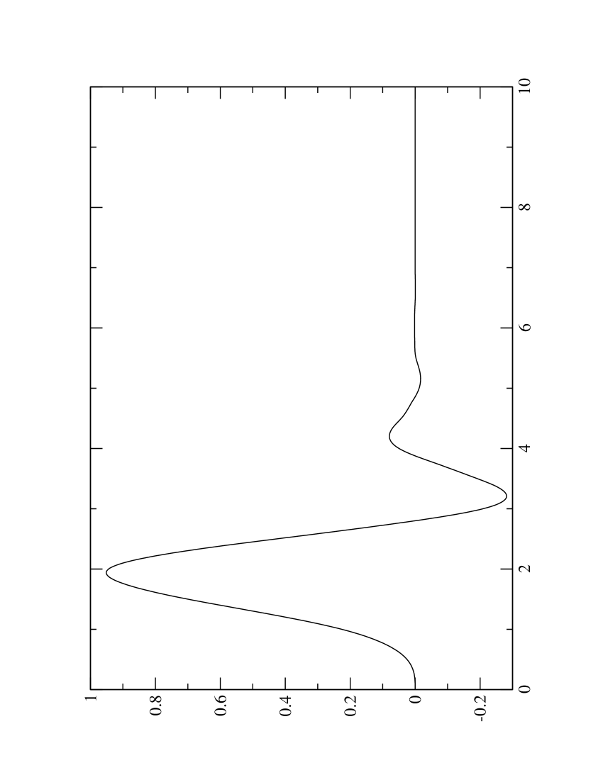
Figure 3: Daubechies’ $K=3$ autocorrelation function.

Using (78) in (76) gives the additional linear constraint on the integrals $\bar{J}_{n}$:

$$-i\pi=-\int^{m}_{-m}{dx\over x-i0^{+}}=$$

$$-\sum_{n}\int^{m}_{-m}dx{\Phi(x+n)\over x-i0^{+}}=$$

$$-\sum_{n}\int^{n+m}_{n-m}dx{\Phi(x)\over x-n-i0^{+}}$$ (79)

which holds for any $m$. Replacing $-i\pi$ on the left side of equation (79) by zero gives the principal value; by $+i0^{+}$ gives the limit on the other side of the real line.

If $m>4K-2$ equation (79) can be expressed as

$$-i\pi=\sum_{n=-m}^{m}\bar{J}_{n}$$

$$+\sum_{n=m+1}^{m+4K-3}\int_{n-m}^{4K-2}{\Phi(x)\over n-x+i0^{+}}dx$$

$$+\sum_{n=-m+1}^{-m+4K-3}\int_{0}^{n+m}{\Phi(x)\over n-x+i0^{+}}dx.$$ (80)

For $|n|>4K-2$ the boundary integrals

$$\int_{n-m}^{4K-2}{\Phi(x)\over n-x+i0^{+}}dx=\int_{n-m}^{\infty}{\Phi(x)\over n-x+i0^{+}}dx$$ (81)

and

$$\int_{0}^{n+m}{\Phi(x)\over n-x+i0^{+}}dx=\int_{-\infty}^{n+m}{\Phi(x)\over n-x+i0^{+}}dx$$ (82)

can be expanded in a convergent power series in terms of partial moments of the autocorrelation function

$$\int_{n-m}^{4K-2}{\Phi(x)\over n-x+i0^{+}}dx={1\over n}\sum_{k=0}^{\infty}{1\over n^{k}}\int_{n-m}^{\infty}\Phi(x)x^{k}dx$$ (83)

and

$$\int_{0}^{n+m}{\Phi(x)\over n-x+i0^{)}}dx={1\over n}\sum_{k=0}^{\infty}{1\over n^{k}}\int_{-\infty}^{n-m}\Phi(x)x^{k}dx$$ (84)

The error after truncating the series in (83) or (84) after $N$ terms is bounded by

$$\left({4K-2\over n}\right)^{N+1}{4K-2\over n-4K+2}\Phi_{max}$$ (85)

where $\Phi_{max}<1$ is the maximum value of the autocorrelation function. It is easy to compute these quantities to machine accuracy. The partial moments of the autocorrelation function in (83) and (84), which are needed as input to (80) can be computed analytically. This calculation is discussed in the appendix.

Equations (74) and (80) can be solved for the $\bar{J}_{n}$ for $0\leq n\leq 4K-2$ in terms of left side of (80), the partial moments of the autocorrelation function, and the integrals for $|n|>4K-2$. The results of these calculations are the nine complex numbers in Table 5. This gives values of $\bar{J}_{m}$ for all $m$. The solution for principal value is given by the real values in table 5, while thc conjugate of the values in table gives the singular integral approaching the real line from the other side.

Table 5 - $\bar{J}_{n}$
m J 0 $-6.400535e-01+i0.000000e+00$ 1 $-1.570288e+00-i7.088321e-01$ 2 $\phantom{-}6.615596e-01-i2.966393e+00$ 3 $\phantom{-}1.719674e+00+i6.560028e-01$ 4 $\phantom{-}6.721642e-02-i1.554882e-01$ 5 $\phantom{-}3.595012e-01+i3.858342e-02$ 6 $\phantom{-}2.261977e-01-i5.023224e-03$ 7 $\phantom{-}1.853414e-01-i4.383938e-04$ 8 $\phantom{-}1.569998e-01-i3.586652e-06$ 9 $\phantom{-}1.357112e-01-i4.424016e-09$ 10 $\phantom{-}1.195044e-01+i0.000000e+00$

The quantity that appears in the integral equation (49) is $J_{mn}(k)$. In order to evaluate this quantity first note that it is symmetric in $m$ and $n$ so we can assume $m\geq n$. For $n\geq 0$ we can express $J_{mn}(k)$ in terms of $\bar{J}_{n}$;

$$J_{mn}(k)=\bar{J}_{k-m-n}.$$ (86)

When either $m$ or $n$ is less than $-2K+2$ then

$$J_{mn}(k)=0$$ (87)

The non-trivial values of $J_{mn}(k)$ correspond to $m$ non-negative and $-2K+2\leq n\leq-1$, and both $-2K+2\leq n,m\leq-1$. This still includes an infinite number of integrals because $k$ can take on any value.

We discuss the treatment of $m$ non-negative and $-2K+2\leq m\leq-1$ separately. When $m$ is non-negative the integral becomes

$$J_{mn}(k)=J_{n}(k-m)$$ (88)

where

$$J_{n}(m):=\int_{0}^{\infty}dx\int_{-\infty}^{\infty}dy{\phi(x-n)\phi(y)\over m-x-y+i0^{+}}.$$ (89)

Because in this case $n$ is within $2K-2$ of zero, for large $|m|$ this can be computed in terms of moments (23) and partial moments (24) of the scaling function using the series method:

$$J_{n}(m)=\sum_{l}{1\over(m-n)^{l+1}}\sum_{k=0}^{l}\langle x^{k}\rangle_{[-n,2K-1]}\langle x^{l-k}\rangle.$$ (90)

The error made by keeping $N$ terms in the $l$ sum is bounded by

$$\left({2K-1\over m-n}\right)^{N+1}{(2K-1)^{2}\over m-n-2K+1}(\phi_{max})^{2}$$ (91)

which can be made as small as desired by choosing a large enough $m$.

Using (64) in (89) gives

$$J_{n}(m)=\sum_{l=0}^{2K-1}\sum_{l^{\prime}=0}^{2K-1}h_{l}h_{l^{\prime}}J_{2n+l}(2m-l^{\prime})$$ (92)

relations among these integrals for different values of $m$ and $n$. Equation (92) can be used to recursively step down from large values of $|m|$ to $m=-1$ from below and $m=2K$ from above. Some terms in this recursion will be complex because they involve the integrals $\bar{J}_{n}$ for $1\leq n\leq 4K-3$.

The values of $J_{n}(m)$ that cannot be computed directly from the moments or by using the recursion correspond $-2K+2\leq n\leq-1$ and $0\leq m\leq 2K-1$. These can be computed by treating (92) as a system of linear equations for the unknown $J_{n}(m)$s. This works because the terms in (92) include some of the previously computed integrals. The results of this calculation are shown in Table 6.

Table 6 - $J_{m}(n)$
m n $J$ -4 0 $-5.270534e-05+i0.000000e-00$ -4 1 $\phantom{-}1.328492e-04-i1.360295e-03$ -4 2 $\phantom{-}4.129155e-04+i3.906821e-04$ -4 3 $-9.487772e-05-i9.892161e-05$ -4 4 $\phantom{-}3.178448e-06-i1.800341e-06$ -4 5 $\phantom{-}1.039698e-07-i6.117942e-09$ -3 0 $-4.625359e-03+i0.000000e-00$ -3 1 $-2.620525e-03-i5.640861e-02$ -3 2 $\phantom{-}2.569291e-02+i1.368533e-02$ -3 3 $-2.507103e-04-i2.505784e-03$ -3 4 $-1.189214e-03-i3.325919e-04$ -3 5 $\phantom{-}8.403857e-05+i4.945118e-06$ -2 0 $\phantom{-}5.719523e-02+i0.000000e-00$ -2 1 $\phantom{-}8.006177e-02+i3.624922e-01$ -2 2 $-2.606313e-01-i7.778517e-02$ -2 3 $\phantom{-}3.145142e-02+i2.488590e-02$ -2 4 $-1.188904e-02-i5.439550e-03$ -2 5 $-9.599595e-03-i4.332178e-04$ -1 0 $-2.730099e-01+i0.000000e-00$ -1 1 $-4.302964e-01-i1.483101e+00$ -1 2 $\phantom{-}1.269047e+00+i2.936519e-01$ -1 3 $-2.565108e-01-i9.893945e-02$ -1 4 $\phantom{-}1.173431e-01+i4.010587e-02$ -1 5 $\phantom{-}4.476128e-02-i5.054775e-03$

What remains are the $J_{mn}(k)$ when both $m$ and $n$ fall between $-2K+2$ and $-1$. In this case when $|k|$ is large, $J_{mn}(k)$ can be expressed in the form of a convergent power series in terms of moments and partial moments of the scaling function. The scaling equations can be used to step up or down in $k$ until $k$ is between $0$ and $2K-2$; in addition they can also be used to solve for cases when

$$m,n,k\in[-2K+2,-1]\times[-2K+2,-1]\times[0,2K-1].$$ (93)

In a normal application the value $k$ represents the on-shell energy. It will be large if there are a lot of basis functions with support on either side of the on-shell point. While $J_{mn}(k)$ can be calculated at the points (93) from the known values using the scaling equation (92), these points do not arise in most applications.

This completes the computation of the singular integrals that appear in equation (49).

V Conclusion

In this paper we introduced a method for applying wavelet numerical analysis to solve the relativistic three-body problem. The method starts by making variable changes in the relativistic Faddeev-Lovelace equations so the moving scattering singularity has simple scaling properties.

The next step is to project the equation in the transformed variables on a finite resolution subspace of the three-body Hilbert space. The matrix representation of the integral equation in this approximation space is easily computed by evaluating the driving terms and smooth part of the kernel at the one-point quadrature points. Additional integrals involving the singular part of the kernel over the basis functions are needed to compute the full kernel. These integrals can be calculated either exactly or with precisely controlled errors using the scaling equation (1) and normalization condition (2). Method for computing all of the required integrals are discussed in detail in section IV and the appendix. Explicit values of most of the needed integrals are computed and appear in Tables 3-6. The physics input is in the driving term and smooth part of the kernel. The integrals over the singular part of the kernel are independent of the dynamics. They can be computed from the scaling coefficients by solving a small system of linear equations.

The resulting system of equations in the high resolution basis, while easy to compute, is large. The wavelet transform is used to transform matrix elements in the high-resolution scaling basis to matrix elements in a basis consisting of low resolution scaling functions and wavelet basis functions with resolutions that fall between the high-resolution and low resolution basis. The transformation to this new basis take $O(N)$ steps, which is faster than a fast Fourier transform. In the new basis the kernel can naturally be expressed as the sum of a sparse matrix and a small matrix. The key approximation is to replace the small part of the kernel by zero. The size of the error made in this approximation can be controlled by changing the threshold size for discarding matrix elements.

The sparse matrix can be solved using sparse matrix techniques. In reference kessler04 this was done by first conditioning the matrix and then using the complex bi-conjugate gradient method. The resulting solution can be transformed back to the scaling basis using the inverse wavelet transform. The approximation is improved if the resulting solution is substituted back in the original equation Sloan . The step has the added benefit that the basis functions never have to be calculated.

The key result that was needed to calculate integrals associated with the moving singularities is the observation by Beylkin beylkin1 beylkin2 beylkin3 and collaborators that integrals of scaling functions over moving singularities can be expressed as integrals of the autocorrelation function of the scaling function over a fixed singularity. This leads to a practical and stable method for computing the integrals. The methods do not require subtractions or careful choices of quadrature points; for the Daubechies’ $K=3$ basis they are reduced to solving a system of eleven linear equations. The required properties of the autocorrelation function are derived in the appendix.

The research in references kessler03 and kessler04 demonstrated that the wavelet method led to sparse matrix approximations resulting negligible errors. The structure of the kernel in the relativistic three-body case indicates that the wavelet method will lead to accurate sparse matrix approximations to the relativistic Faddeev-Lovelace equations.

The increase in efficiency in this method is due to the saving in computational effort in going from solving a large dense set of linear equations to an approximately equivalent equations with a sparse matrix. The wavelet method will lead to a significant savings in computational effort for a large system.

Our conclusion is that wavelet numerical analysis can be used to accurately approximate the relativistic Faddeev Lovelace equations by a linear system of equations with a sparse kernel matrix.

Appendix A

The autocorrelation function of the scaling function is defined by

$$\Phi(x)=\int^{\infty}_{-\infty}\phi(x-y)\phi(y)dy.$$ (94)

Because of the support of the scaling function is $[0,2K-1]$, the autocorrelation function has support $[0,4K-2]$.

Using the scaling equation (64) for the scaling function in the definition (94) of the autocorrelation function leads to the scaling equation for the autocorrelation function:

$$\Phi(x)=\sum_{l}\sum_{l^{\prime}}h_{l}h_{l^{\prime}}\Phi(2x-l^{\prime}-l).$$ (95)

If we define

$$a_{l}={1\over\sqrt{2}}\sum_{l^{\prime}=0}^{min(l,2K-1)}h_{l-l^{\prime}}h_{l^{\prime}}\qquad 0\leq l\leq 4K-2$$ (96)

equation (95) can be put in the same form as (1):

$$D\Phi(x)=\sum_{l=0}^{4K-2}a_{l}T^{l}\Phi(x).$$ (97)

The scaling coefficients $a_{k}$ for the Daubechies’ $K=3$ autocorrelation function are given in Table 7.

Table 7: Daubechies’ $K=3$ Autocorrelation Scaling Coefficients
$a_{0}$ $\phantom{-}7.825529e-02$ $a_{1}$ $\phantom{-}3.796160e-01$ $a_{2}$ $\phantom{-}6.767361e-01$ $a_{3}$ $\phantom{-}4.612557e-01$ $a_{4}$ $-4.471656e-02$ $a_{5}$ $-1.687321e-01$ $a_{6}$ $-2.481571e-03$ $a_{7}$ $\phantom{-}3.922363e-02$ $a_{8}$ $-1.563883e-03$ $a_{9}$ $-4.256471e-03$ $a_{10}$ $\phantom{-}8.774429e-04$

Table 8: Daubechies’ $K=3$ Autocorrelation Moments
$\langle x^{0}\rangle_{\Phi}$ $1.000000e+00$ $\langle x^{1}\rangle_{\Phi}$ $1.634802e+00$ $\langle x^{2}\rangle_{\Phi}$ $2.672579e+00$ $\langle x^{3}\rangle_{\Phi}$ $4.167773e+00$ $\langle x^{4}\rangle_{\Phi}$ $5.825913e+00$ $\langle x^{5}\rangle_{\Phi}$ $6.817542e+00$ $\langle x^{6}\rangle_{\Phi}$ $8.807917e+00$ $\langle x^{7}\rangle_{\Phi}$ $4.055470e+01$ $\langle x^{8}\rangle_{\Phi}$ $2.899550e+02$ $\langle x^{9}\rangle_{\Phi}$ $1.695851e+03$ $\langle x^{10}\rangle_{\Phi}$ $8.321402e+03$

The normalization condition (1) of the scaling function can be used in the definition (94) of the autocorrelation function to derive the normalization condition:

$$\int\Phi(x)dx=1.$$ (98)

The scaling equation (95) and the normalization condition (98) can be used calculate moments and partial moments of the autocorrelation function. To calculate the moments of the autocorrelation function use

$$\langle x^{k}\rangle_{\Phi}=\int\Phi(x)x^{k}dx,$$ (99)

$$\langle x^{k}\rangle_{\Phi}={1\over 2^{k+1/2}}\sum_{l}a_{l}\sum_{n=0}^{k}{k!\over n!(k-n)!}l^{n-k}\langle x^{n}\rangle_{\Phi}.$$ (100)

Moving the $n=k$ term to the left side of the equation gives recursion relation

$$\langle x^{k}\rangle_{\Phi}:={1\over 2^{k}-1}{1\over\sqrt{2}}\sum_{l}a_{l}\sum_{n=1}^{k}{k!\over n!(k-n)!}l^{n}\langle x^{k-n}\rangle_{\Phi}.$$ (101)

The recursion is started using the the normalization condition (98). The lowest moments are tabulated in Table 8.

The partial moments of the autocorrelation function satisfy the scaling equation

$$\langle x^{k}\rangle_{\Phi,[m,\infty]}:=\int_{m}^{\infty}\Phi(x)x^{k}dx=$$

$$\sum_{l}a_{l}\sum_{n=0}^{k}{\sqrt{2}\over 2^{k+1}}{k!\over n!(k-n)!}l^{m}\langle x^{k-m}\rangle_{\Phi,[2m-l,\infty]}.$$ (102)

When $m\geq 4K-2$ these partial moments become ordinary moments while when $m\leq 0$ they vanish. This gives us a linear system for partial moments in terms of the full moments and lower partial moments. These equations can be solved recursively. Partial moments corresponding to more general intervals can be computed by subtraction:

$$\langle x^{k}\rangle_{\Phi,[m,n]}=\langle x^{k}\rangle_{\Phi,[m,\infty]}-\langle x^{k}\rangle_{\Phi,[n,\infty]}.$$ (103)

References

- (1) B. M. Kessler, G. L. Payne, W. N. Polyzou, Few-Body Systems, 33,1(2003), nucl-th/0211016.
- (2) B. M. Kessler, G. L. Payne, W. N. Polyzou, Phys. Rev. C70,034003(2004), nucl-th/0406079.
- (3) See http:www.jpeg.org.
- (4) V. G. J. Stoks, R. A. M. Klomp, C. P. F. Terheggen, J. J. de Swart, Phys. Rev. C49,2950(1994).
- (5) R. B. Wiringa, V. G. J. Stoks, R. Schiavilla, Phys. Rev. C51,38(1995), nucl-th/9408016.
- (6) R. Machleit, (2000), nucl-th/0006014
- (7) Steven C. Pieper, R. B. Wiringa, Ann. Rev. Nucl. Part. Sci. 51,53(2001), nucl-th/0103005.
- (8) H. Witala, J. Golak, W. Glöckle, and H. Kamada, Phys. Rev. C71,054001(2005).
- (9) B. D. Keister and W. N. Polyzou in Advances in Nuclear Physics Volume 20, Ed. J. W. Negele and E.W. Vogt ( Plenum Press, New York, 1991).
- (10) W. N. Polyzou J. Math. Phys. 43,6024(2002), nucl-th/0201013.
- (11) Michael G. Fuda, Hamoud Alharbi, Phys. Rev. C68,064002(2003).
- (12) W. N. Polyzou, Phys. Rev. C68,015202(2003), nucl-th/0302023.
- (13) F. Coester, Helv. Phys. Acta, 38,7(1965).
- (14) R. A. Malfliet and J. A. Tjon, Nucl. Phys. A27,161(1969).
- (15) G. L. Payne, J. L. Friar, B. F. Gibson, and I. R. Afnan, Phys. Rev. C22, 823(1980).
- (16) Ingrid Daubechies, Comm. on Pure and Applied Mathematics Vol. XLI, 909-996(1988).
- (17) Ingrid Daubechies,Ten Lecture on Wavelets (SIAM, Philadelphia, PA, 1992)
- (18) G. Kaiser, A Friendly Guide to Wavelets (Birkhäuser, Boston, 1994).
- (19) H. L. Resnikoff and R. O. Wells, Wavelet Analysis: The Scalable Structure of Information (Springer-Verlag, New York, 1998).
- (20) G. Strang, SIAM Review, 31 4,614(1989).
- (21) O. Bratelli and P. Jorgensen, Wavelets Through a Looking Glass, The World of the Spectrum (Birkhäuser. Boston, 2002).
- (22) B. M. Kessler, G. L. Payne, W. N. Polyzou Wavelet Notes, nucl-th/0305025.
- (23) W. H. Press, S. A. Teukolsky, W. T. Vettering, B. P. Flannery, Numerical Recipes in C (Cambridge University Press, Cambridge, 1992).
- (24) G. H. Golub, C. F. Van Loan, Matrix Computations, (Johns Hopkins University Press, Baltimore, 1996).
- (25) I. Sloan, Math. Comp. 30,758(1976).
- (26) W.-C. Shann, Quadrature rules needed in Galerkin-wavelets methods, Proceedings for the 1993 annual meeting of Chinese Mathematics Association(Chiao-Tung Univ, Dec., 1993), http://www.math.ncu.edu.tw/ shann/Math/pre.html
- (27) W.-C. Shann and J.-C. Yan, Quadratures involving polynomials and Daubechies’ wavelets. Technical Report 9301 (Department of Mathematics, National Central University 1993), http://www.math.ncu.edu.tw/ shann/Math/pre.html.
- (28) W. Sweldens and R. Piessens, SIAM J. Numer. Anal., 31,1240(1994).
- (29) G. Beylkin, SIAM Journal on Numerical Analysis, 29,6,1716(December, 1992)
- (30) G. Beylkin and N. Saito, “ Wavelets, their autocorrelation functions, and multiresolution representation of signals”, D.P.Casasent (Ed.), Proc. SPIE: Intelligent Robots and Computer Vision XI: Biological, Neural Net, and 3D Methods, Vol. 1826, SPIE,39(1992).
- (31) N. Saito, G. Beylkin, IEEE Transactions on Signal Processing, 41,12,3584(1993).