EVOLUTION OF OBSERVABLES IN A NUMERICAL KINETIC MODEL.

Abstract

The numerical solutions of the nonrelativistic and relativistic Boltzmann equations have been studied at various initial conditions. Particularly, the known analytical solution of the nonrelativistic Boltzmann equation at spherically symmetric Gaussian initial conditions has been recovered and the corresponding conservation of particle spectra and correlation functions has been confirmed. Similar conservation properties have been found also for a more general class of solutions describing the nonrelativistic and relativistic systems at anisotropic initial conditions.

I Introduction.

The evolution of the matter formed in ultrarelativistic heavy ion collisions is usually described within hydrodynamic and transport models. The former allow one to incorporate the complicated evolution of the hot and dense system (fireball) at the possible phase transitions encoded in corresponding equation of state, while the latter make it possible to evaluate particle spectra taking into account the nonequilibrated character of their formation even at the early evolution stage. However, in realistic conditions, neither of these approaches nor their hybrids are able to reproduce particle spectra and correlations in A+A collisions. At present there is no scenario of the evolution allowing one to describe all the salient features of hadronic observables, including the interferometry or correlation radii related to the space-time scales of the fireball. Particularly, the observed approximate energy independence of the radii is considered as the interferometry puzzle.

It was noted Sinyukov , based on an analysis of the exact solution of the nonrelativistic Boltzmann equation exact ; CCL98 , that under specific conditions which could be realized at the moment when fireball starts to decay, e.g., at the end of the pure hydrodynamic stage of the matter evolution, spectra and interferometry radii may become “frozen” at this early moment despite the particle emission and collisions between hadrons last for a fairly long period of the system decay. It was also proposed Sinyukov that this peculiar theoretical result can be used to test numerical transport models of A+A collisions and this is one of the aims of this paper. Another aim is a study, within kinetic approach, to what extent is the conservation of spectra and interferometry radii violated during the system evolution in the case of more realistic initial conditions. This study is particularly interesting in the context of recently observed akksin approximate conservation of interferometry volume during isentropic and chemically frozen hydrodynamic evolution of hadron-resonance gas and, it can be quite useful to solve the interferometry puzzle.

The analysis of above phenomena has been done within Universal Kinetic Model (UKM) Am2002 , a Monte Carlo event generator, realized as a numerical code written in object oriented C++ language. The UKM gives a possibility to model kinetic processes inside a particle system applying a suitable numerical algorithm. This model is a universal one, since there is a possibility to choose and add particle system (e.g., system of hadrons, system of partons, etc.) and to choose and add a particular numerical algorithm, i.e., to choose and add different kinetic modeler. In our studies, we have used a cascade version of the UKM code, UKM-R UKMRoot , written under the ROOT system ROOT . We use the same numerical cascade algorithm as implemented in the Quark Gluon String model AGTS90 .

The paper is now organized as follows. In section II we relate particle spectra and two–particle correlation function with distribution and emission functions. Section III deals with the theoretical aspects of the spectra formation, including a possible duality between kinetic and hydrodynamic approaches. Section IV is devoted to a brief UKM-R description. In section V we discuss the known exact solution of the nonrelativistic Boltzmann equation for an expanding fireball with the spherically symmetric Gaussian initial conditions. This solution is used in section VI to test the UKM-R. Section VII deals with the influence of anisotropic initial conditions and relativistic effects on the final spectra and interferometry radii. The results are summarized in section VIII.

II Distribution and emission functions.

The inclusive particle spectra are related to the averages of the products of creation and annihilation operators, $a_{p}^{+}$ and $a_{p}$, calculated at sufficiently large time $t_{\mbox{\scriptsize out}}$ or, generally, on an asymptotic hypersurface $\sigma_{\mbox{\scriptsize out}}:t=t_{\mbox{\scriptsize out}}(\mathbf{x})$, guaranteeing the absence of further interactions. Thus

$$p^{0}\frac{d^{3}N}{d^{3}\mathbf{p}}\equiv n(p)=\langle a_{p}^{+}a_{p}\rangle,~{}~{}~{}~{}~{}p_{1}^{0}p_{2}^{0}\frac{d^{6}N}{d^{3}\mathbf{p\mathtt{{}_{1}}}d^{3}\mathbf{p}\mathtt{{}_{2}}}\equiv n(p_{1},p_{2})=\langle a_{p_{1}}^{+}a_{p_{2}}^{+}a_{p_{1}}a_{p_{2}}\rangle.$$ (1)

In the case of independent (chaotic) particle production and subsequent system kinetic evolution, one can express the average of the product of four operators through the irreducible averages $\langle a_{p}^{+}a_{p^{\prime}}\rangle$, similar to Wick theorem for thermal systems. For identical spin-0 bosons

$$n(p_{1},p_{2})=\langle a_{p_{1}}^{+}a_{p_{1}}\rangle\langle a_{p_{2}}^{+}a_{p_{2}}\rangle+\langle a_{p_{1}}^{+}a_{p_{2}}\rangle\langle a_{p_{2}}^{+}a_{p_{1}}\rangle.$$ (2)

In kinetic approach, the irreducible averages are expressed through the integrals or Fourier transforms of the distribution function $f(x,p)$ on the hypersurface $\sigma_{\mbox{\scriptsize out}}$:

$$\langle a_{p}^{+}a_{p}\rangle=\int_{\sigma_{\mbox{\scriptsize out}}}d^{3}\sigma_{\mu}(x)p^{\mu}f(x,p),~{}~{}~{}\langle a_{p_{1}}^{+}a_{p_{2}}\rangle=\int_{\sigma_{\mbox{\scriptsize out}}}d^{3}\sigma_{\mu}(x)p^{\mu}e^{-iqx}f(x,p),$$ (3)

where, in the nondiagonal average in the second integral, $p=(p_{1}+p_{2})/2$ is an off-mass-shell four-momentum and $q=p_{1}-p_{2}$. The actual choice of $t_{\mbox{\scriptsize out}}$ does not matter due to the current conservation for free streaming particles and, due to the fact that, as a consequence of the relation $qp=0$, the four-vector product $qx$ is independent of the position $x$ on the trajectory of a free off-mass-shell particle with four-momentum $p$ (i.e., $qx$ is invariant with respect to transformations $t\to t+\delta t$ and $\mathbf{x}\to\mathbf{x}+(\mathbf{p}/p^{0})\delta t$).

The distribution function $f(x,p)$ is closely related with the current emission function $S^{\sigma}(\bar{x},p)$ on a hypersurface $\sigma:t=t({\bf x})$ since it collects contributions of the emission or scattering points $\bar{x}=\{\bar{t},\mathbf{x}-(\mathbf{p}/p^{0})(t-\bar{t})\}$ starting from those free particles with the three-velocity $\mathbf{p}/p^{0}$ reach a point $x=\{t,\mathbf{x}\}$. Particularly, choosing the hypersurface $\sigma:t=const$, one has

$$p^{0}f(x,p)=\int d^{4}\bar{x}\,\delta^{3}\left(\bar{\mathbf{x}}-\mathbf{x}+(\mathbf{p}/p^{0})(t-\bar{t})\right)S^{\sigma}(\bar{x},p).$$ (4)

Inserting Eq. (4) into Eq. (3) and using the equality $q\bar{x}=qx$, one can rewrite the asymptotic operator averages as four-volume integrals or Fourier transforms of the asymptotic emission function $S(\bar{x},p)\equiv S^{\sigma_{\mbox{\scriptsize out}}}(\bar{x},p)$ als02 :

$$\langle a_{p}^{+}a_{p}\rangle=\int d^{4}\bar{x}S(\bar{x},p),~{}~{}~{}\langle a_{p_{1}}^{+}a_{p_{2}}\rangle=\int d^{4}\bar{x}e^{-iq\bar{x}}S(\bar{x},p).$$ (5)

Using Eqs. (1)-(5), one can write the two-boson correlation function (CF) as

$${\cal R}(p_{1},p_{2})\equiv\frac{n(p_{1},p_{2})}{n(p_{1})n(p_{2})}=1+|{\cal F}(p,q))|^{2}=1+\langle\cos(qx_{12})\rangle^{\prime},$$ (6)

where $x_{12}=x_{1}-x_{2}$,

$${\cal F}(p,q)=\frac{\langle a_{p_{1}}^{+}a_{p_{2}}\rangle}{[\langle a_{p_{1}}^{+}a_{p_{1}}\rangle\langle a_{p_{2}}^{+}a_{p_{2}}\rangle]^{1/2}}$$ (7)

and the quasiaverage

$$\langle\cos(qx_{12})\rangle^{\prime}=\frac{\int d^{3}\sigma_{\mu}(x_{1})d^{3}\sigma_{\nu}(x_{2})p^{\mu}p^{\nu}f(x_{1},p)f(x_{2},p)\cos(qx_{12})}{\int d^{3}\sigma_{\mu}(x_{1})d^{3}\sigma_{\nu}(x_{2})p_{1}^{\mu}p_{2}^{\nu}f(x_{1},p_{1})f(x_{2},p_{2})}$$

$$=\frac{\int d^{4}\bar{x}_{1}d^{4}\bar{x}_{2}\,\cos(q\bar{x}_{12})\,S\left(\bar{x}_{1},p\right)S\left(\bar{x}_{2},p\right)}{\int d^{4}\bar{x}_{1}\,S\left(\bar{x}_{1},p_{1}\right)\int d^{4}\bar{x}_{2}\,S\left(\bar{x}_{2},p_{2}\right)}.$$ (8)

Obviously, the CF decreases from 2 at $q=0$ to unity at large $|q^{\mu}|$ and the width of this Bose-Einstein enhancement is inversely related to the effective system size which is usually encoded in so called interferometry radii.

In this paper, we will also use Eqs. (1)-(8) to calculate spectra and CF’s at any earlier evolution times $t_{\sigma}<t_{\sigma_{\mbox{\scriptsize out}}}$ on a hypersurface $\sigma$. To do so, one has to make only the substitutions $\sigma_{\mbox{\scriptsize out}}\to\sigma$ and $S(\bar{x},p)\to S^{\sigma}(\bar{x},p)$. Note that the current emission function $S^{\sigma}(\bar{x},p)$ takes into account the kinetic evolution up to the evolution time $t_{\sigma}$ only and satisfies the obvious relations: $S^{\sigma}(\bar{x},p)\geq S(\bar{x},p)$ for $\bar{t}\leq t_{\sigma}$ and $S^{\sigma}(\bar{x},p)=0$ for $\bar{t}>t_{\sigma}$. Particularly, for a system of noninteracting particles the emission function is independent of the evolution time and the asymptotic one, $S(\bar{x},p)$, coincides with that, $S^{\sigma_{0}}(\bar{x},p)$, determined on the initial hypersurface $\sigma_{0}:~{}t=t_{0}(\mathbf{x})$.

To calculate the kinetic evolution, we will use the simple ansatz $S^{\sigma_{0}}(\bar{x},p)=p^{0}f(\bar{x},p)\delta(\bar{t})$ for the initial emission function on the hypersurface $\sigma_{0}:~{}t=0$. Though this ansatz generally violates the uncertainty relation $\Delta\bar{t}\cdot\Delta p^{0}\geq 1$, it causes no problem since the evolution initial condition is determined by the initial distribution function only and since there exist a whole family of the initial emission functions of a finite time width recovering the latter in accordance with Eq. (4).

III Theoretical aspects of the spectra formation.

The distribution function describes an expanding system of interacting particles and satisfies Boltzmann equation (BE) which, in the case of no external forces, has the form:

$${p^{\mu}}\frac{\partial f(x,p)}{\partial x^{\mu}}=C_{\mbox{\scriptsize gain}}(x,p)-C_{\mbox{\scriptsize loss}}(x,p).$$ (9)

The collision terms $C_{\mbox{\scriptsize gain}}$ and $C_{\mbox{\scriptsize loss}}$ are associated with the numbers of particles that respectively come to the phase space point $(x,p)$ and leave this point because of collisions. Let us follow Ref. Sinyukov and split the distribution function at each space-time point $x$ into two terms: $f(x,p)=f_{\mbox{\scriptsize int}}(x,p)+f_{\mbox{\scriptsize esc}}(x,p)$. The first one, $f_{\mbox{\scriptsize int}}(x,p)$, describes the particles continuing to interact after the time $t$. The second one, $f_{\mbox{\scriptsize esc}}(x,p)$, describes the particles that do not interact any more after the time $t$. Introducing escape probability $P(x,p)$, i.e., the probability that any given particle at phase space point $(x,p)$ does not interact any more and propagates freely, one can write

$$f_{\mbox{\scriptsize esc}}(x,p)=P(x,p)\,f(x,p).$$ (10)

At large enough times $t\sim t_{\mbox{\scriptsize out}}$, $P(x,p)\rightarrow 1$ and $f_{\mbox{\scriptsize esc}}(x,p)\rightarrow f(x,p)$. Since in the evolution of $f_{\mbox{\scriptsize esc}}(x,p)$ there is no loss of particles and the gain is associated with the part of the emission function, $S_{\mbox{\scriptsize g}}(x,p)=[1-\theta(t_{0}-t)]S(x,p)$, developed during the kinetic evolution starting at a hypersurface $\sigma_{0}$ and describing particles suffering last collisions at space-time point $x$, the escape function satisfies the following BE Sinyukov :

$$p^{\mu}\frac{\partial}{\partial x^{\mu}}f_{\mbox{\scriptsize esc}}(x,p)=P(x,p)C_{\mbox{\scriptsize gain}}(x,p)\,\equiv S_{\mbox{\scriptsize g}}(x,p).$$ (11)

Noting that $\partial_{\mu}[p^{\mu}\exp{(-iqx)}]=0$ and that $f_{\mbox{\scriptsize esc}}(x,p)=f(x,p)$ on the asymptotic hypersurface ${\sigma_{\mbox{\scriptsize out}}}$, one obtains, applying the Gauss theorem to the Fourier transform of the distribution function in Eq. (3) and using respectively general equations (11) and (9) analytically continued to off-mass-shell four-momenta $p$:

$$\langle a_{p_{1}}^{+}a_{p_{2}}\rangle=\int_{\sigma_{0}}d^{3}\sigma_{\mu}(x_{0})p^{\mu}f_{\mbox{\scriptsize esc}}(x_{0},p)e^{{-iqx_{0}}}+\int_{\sigma_{0}}^{\sigma_{\mbox{\scriptsize out}}}\!d^{4}x\,S_{\mbox{\scriptsize g}}(x,p)e^{{-iqx}},$$ (12)

$$\langle a_{p_{1}}^{+}a_{p_{2}}\rangle=\int_{\sigma_{0}}d^{3}\sigma_{\mu}(x_{0})p^{\mu}f(x_{0},p)e^{{-iqx_{0}}}+\int_{\sigma_{0}}^{\sigma_{\mbox{\scriptsize out}}}d^{4}x\,\left[C_{\mbox{\scriptsize gain}}(x,p)\!-\!C_{\mbox{\scriptsize loss}}(x,p)\right]e^{{-iqx}},$$ (13)

where $S_{\mbox{\scriptsize g}}(x,p)=PC_{\mbox{\scriptsize gain}}$ is defined in Eq. (11), $f_{\mbox{\scriptsize esc}}(x_{0},p)$ corresponds to the portion of the particles that are already free at initial time $t_{0}$ (generally, at initial hypersurface $\sigma_{0}$) and $f(x_{0},p)$ is the distribution function at $\sigma_{0}$. Thus, as stated in Eqs. (3) and (5), the Fourier transform of the distribution or escape function on the asymptotic hypersurface $\sigma_{\mbox{\scriptsize out}}$ is equivalent to the four-volume Fourier transform of the emission function, the latter being represented by the emission function $S_{\mbox{\scriptsize g}}=PC_{\mbox{\scriptsize gain}}$ developed during the kinetic evolution starting from the initial hypersurface $\sigma_{0}$, together with the emission function $\theta(t_{0}-\bar{t})S(\bar{x},p)$ corresponding to emission times $\bar{t}\leq t_{\sigma_{0}}$. The latter determines the escape function $f_{\mbox{\scriptsize esc}}(x_{0},p)$ on the hypersurface $\sigma_{0}$ through Eq. (4) modified by the substitutions $f\to f_{\mbox{\scriptsize esc}},~{}S^{\sigma}\to\theta(t_{0}-\bar{t})S(\bar{x},p)$.

One may see from Eq. (13) that for a quasifree system characterized by the equality $C_{\mbox{\scriptsize gain}}=C_{\mbox{\scriptsize loss}}$, the spectra and correlations are not affected by the kinetic evolution and are completely determined by the initial distribution function. An example is the system of nonrelativistic particles with the initial spherically symmetric Gaussian distribution function Sinyukov ; CCL98 .

In hydrodynamic approach, the Landau freeze-out criterion of locally equilibrium (leq) hydrodynamic momentum spectra and corresponding Cooper-Frye prescription, defined by Eq. (3) with substitutions $\sigma_{\mbox{\scriptsize out}}\!\rightarrow\sigma_{\mbox{\scriptsize f}}$ and $f\!\rightarrow f_{\mbox{\scriptsize leq}}$, treats particle spectra as a result of rapid conversion of a hadron system in local equilibrium into a gas of free particles on some freeze-out hypersurface $\sigma_{\mbox{\scriptsize f}}$. Formally, it corresponds to taking the cross section tending to infinity at $t<t_{\sigma_{\mbox{\scriptsize f}}}$ (to keep the system in local equilibrium) and zero beyond $t_{\sigma_{\mbox{\scriptsize f}}}$. Then $C_{\mbox{\scriptsize gain}}=C_{\mbox{\scriptsize loss}}$, $P(x,p)=\theta(t-t_{\sigma_{\mbox{\scriptsize f}}})$, $f_{\mbox{\scriptsize esc}}=\theta(t-t_{\sigma_{\mbox{\scriptsize f}}})f_{\mbox{\scriptsize leq}}$ and $S=p^{0}\delta(t-t_{\sigma_{\mbox{\scriptsize f}}})f_{\mbox{\scriptsize leq}}$. However, as stressed in Ref. Borysova , in the realistic case of continuous freeze-out the emission function $S(x,p)$ is no more proportional to the distribution function $f(x,p)$. At the same time, the spectra and the interferometry radii can be simply determined using the Cooper-Frye prescription for the fireball characterized by the thermal distribution function at the moment before it starts to emit particles and decays. As analyzed in detail in Ref. Sinyukov , such a duality between hydrodynamic and transport approaches can happen when the integral of the difference $C_{\mbox{\scriptsize gain}}-C_{\mbox{\scriptsize loss}}$ in Eq. (13) vanishes, as is the case for a system of nonrelativistic particles with the initial spherically symmetric Gaussian distribution function (see sections V and VI), or, when this integral is small, what can happen for a more wide class of initial conditions (see section VII).

IV Universal kinetic model.

In our studies, we have used the UKM-R code UKMRoot written under ROOT system. In this code one deals with particle objects and their lists. Any particle object has its static and dynamic attributes. The static attributes are such as particle names, charges, masses or widths. The dynamic attributes are particle four-coordinates and four-momenta. The particle objects are grouped into particle lists. The ROOT classes are used to describe particle properties, to operate with three- and four-vectors and to organize containers.

In the present work, we have considered only one type of particles and taken into account only their elastic binary collisions. We have thus created a specific list of primary particles specifying their spatial and momentum distributions and derived the Elastic interaction and Cascade model classes from the respective UKM Particle interaction and Universal kinetic algorithm ones. The Cascade model class represents the BE solver. The used UKM-R deals with the following lists:

(i) Primaries, (ii) Collisions, (iii) Secondaries, (iv) New secondaries
and the following basic classes:

(i) Initial state, (ii) Elastic interaction, (iii) Cascade model.

The numerical algorithm AGTS90 can be described as follows:

1. The list of primaries is initialized and an initial value of the current time is set.

2. At first, all possible pairs of colliding particles from the primaries list are searched for and the collision list is filled in according to the increasing collision time. The binary particle collision is considered as possible whenever the distance $d$ of closest approach of the two particles in their c.m. system is less than the collision distance calculated from the total collision cross section which is a function of the two–particle c.m. energy $\sqrt{s}$, i.e.,

   $$d<\left[{\sigma\left(\sqrt{s}\right)/{\pi}}\right]^{1/2}.$$ (14)

   In the present study, only elastic scattering is considered and a constant test cross section is used.

3. The earliest collision is simulated, the two collided particles are removed from all lists and the created particles are put in the list of new secondaries. The particle coordinates are shifted in accordance with the time of simulated collision and particle velocity vectors.

4. The collisions of the particles from new secondaries list with all particles from primaries and secondaries lists are searched for and the time ordered collision list is updated.

5. The content of new secondaries list is moved to secondaries list and simulation continues starting from step 3 or stops when the collision list is empty or the current time exceeds the user defined value of the stop time.

It should be noted that the above algorithm violates the Lorentz covariance Covariance98 since the condition $(\ref{B5})$ introduces action at distance and breaks local character of the BE (see Eqs. (9) and (15)). One can use the invariance of the BE with respect to the transformation $f\rightarrow kf,~{}\sigma\rightarrow\sigma/k$ and diminish nonlocality of the algorithm by simultaneously increasing the number of particles and the inverse interaction cross section by the same factor $k$.

V Exact solution of nonrelativistic BE.

Let us consider the kinetic evolution of a system of $N$ nonrelativistic identical spin-0 particles of mass $m$ assuming the initial conditions corresponding to the global thermal Boltzmann distribution with temperature $T_{0}$ (i.e., the absent initial flow) and spherically symmetric Gaussian profile of particle density with radius $R_{0}$. Assuming further only elastic binary collisions in the system, the collision integral in BE (9) takes the form

$$C_{\mbox{\scriptsize gain}}(x,p)-C_{\mbox{\scriptsize loss}}(x,p)=\int\frac{d^{3}\mathbf{p}_{1}}{2p_{1}^{0}}d\Omega[f(x,p^{\prime})f(x,p_{1}^{\prime})-f(x,p)f(x,p_{1})]F(s)\sigma(\sqrt{s},\theta),$$ (15)

where the particle four-momenta in the binary scattering satisfy the conservation law: $p+p_{1}=p^{\prime}+p^{\prime}_{1}$, $d\Omega=d\cos\theta d\phi$, $\cos\theta=1+2t/(s-4m^{2})$, $s=(p+p_{1})^{2}$, $t=(p-p^{\prime})^{2}$, $F(s)=\frac{1}{2}[s(s-4m^{2})]^{1/2}$ is the invariant flow of two colliding particles of mass $m$ at c.m. energy $\sqrt{s}$ and $\sigma(\sqrt{s},\theta)={d\sigma_{el}}/{d\Omega}$ is the differential cross section of the elastic scattering on the c.m. angle $\theta$. Then, in the nonrelativistic case, the BE has the following analytical solution for the distribution function $f(x,p)\equiv f(t,\mathbf{r},\mathbf{p})$ exact :

$$f(t,\mathbf{r},\mathbf{p})=\frac{N}{\left[2\pi R_{0}(mT_{0})^{1/2}\right]^{3}}\,\exp\left(-\frac{(\mathbf{r}-t\mathbf{p}/m)^{2}}{2R_{0}^{2}}-\frac{\mathbf{p}^{2}}{2mT_{0}}\right).$$ (16)

Since Eq. (16) represents also special case of the solution of hydrodynamic equations for ideal fluid with the radial initial flow, it can be rewritten in the local equilibrium form CCL98 :

$$f(t,\mathbf{r},\mathbf{p})=f_{\mbox{\scriptsize leq}}=\frac{N}{\left[2\pi R_{0}(mT_{0})^{1/2}\right]^{3}}\,\exp\left(-\frac{\mathbf{r}^{2}}{2R^{2}(t)}-\frac{(\mathbf{p}-m\mathbf{u}(t,\mathbf{r}))^{2}}{2mT(t)}\right),$$ (17)

where $T(t)=T_{0}/\varphi(t)$, $R^{2}(t)=R_{0}^{2}\varphi(t)$ and $\mathbf{u}(t,\mathbf{r})=\mathbf{r}\dot{\varphi}(t)/\varphi(t)=\mathbf{r}tT(t)/(mR_{0}^{2})$ are respectively the temperature, the system Gaussian radius squared and the flow velocity, $\varphi(t)=1+T_{0}t^{2}/(mR_{0}^{2})$; the corresponding chemical potential $\mu(t,r)=-\frac{1}{2}T(t)\mathbf{r}^{2}/R^{2}(t)$.

Inserting solution (16) into the BE, one can check that its l.h.s. vanishes, $m{\partial f}/{\partial t}+{\mathbf{p}}{\partial f}/{\partial\mathbf{r}}=0,$ so the collision integral (its r.h.s.) should also vanish. Indeed, inserting the solution (17) into the factor in square brackets in Eq. (15), one can see that the collision integral vanishes (irrespective of energy and angular dependence of the elastic cross section) as a consequence of the energy and three-momentum conservation:

$$[f(x,p^{\prime})f(x,p_{1}^{\prime})-f(x,p)f(x,p_{1})] \propto \exp\left(-\frac{\mathbf{p}^{\prime 2}+\mathbf{p}_{1}^{\prime 2}}{2mT(t)}+\frac{\mathbf{p}^{\prime}+\mathbf{p}_{1}^{\prime}}{T(t)}\mathbf{u}(t,\mathbf{r})\right)$$ (18)

$$- \exp\left(-\frac{\mathbf{p}^{2}+\mathbf{p}_{1}^{2}}{2mT(t)}+\frac{\mathbf{p}+\mathbf{p}_{1}}{T(t)}\mathbf{u}(t,\mathbf{r})\right)=0.$$

This solution thus corresponds to a quasifree motion and so, as discussed in section III (see, e.g., Eq. (13)), the particle spectra and correlations are not affected by the kinetic evolution and stay unchanged at any times Sinyukov ; CCL98 . One may see from Eqs. (16) and (17) that the conservation of the momentum spectrum is related to the fact that the decreasing temperature is compensated by increasing flow velocity. The latter also compensates the effect of increasing system size on the two-boson CF thus guaranteeing the conserved interferometry radius. Indeed, using distribution function (16), explicit calculations yield time-independent momentum spectrum and correlation function:

$$\frac{d^{3}N(t;\mathbf{p})}{d^{3}\mathbf{p}}=\frac{N}{\left(2\pi mT_{0}\right)^{3/2}}\exp\left(-\frac{\mathbf{p}^{2}}{2mT_{0}}\right),$$ (19)

$${\cal R}(t;\mathbf{p}_{1},\mathbf{p}_{2})=1+\exp\left[-\left(R_{0}^{2}-\frac{1}{4mT_{0}}\right)\mathbf{q}^{2}\right],$$ (20)

where $(4mT_{0})^{-1/2}\equiv R_{\mbox{\scriptsize th}}$ measures the characteristic thermal size (heat de Broglie length) of the single-pion emitter. At the same time, as seen from Eq. (17), the system expands and spatial density decreases with increasing time:

$$\frac{d^{3}N(t;\mathbf{r})}{d^{3}\mathbf{r}}=\frac{N}{\left(2\pi R^{2}(t)\right)^{3/2}}\!\exp\left(-\frac{\mathbf{r}^{2}}{2R^{2}(t)}\right),$$ (21)

where $R^{2}(t)=R_{0}^{2}+t^{2}T_{0}/m$.

VI Test of the UKM-R algorithm.

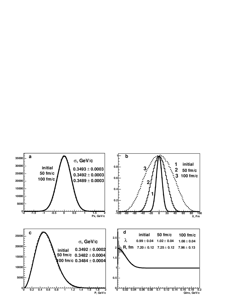
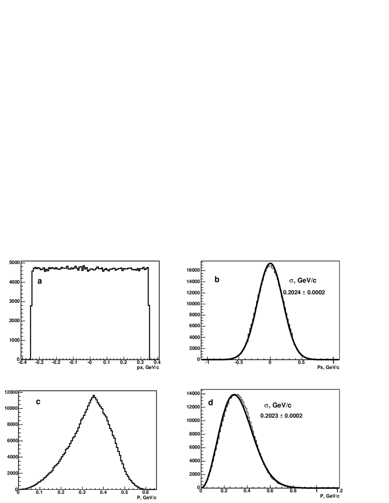
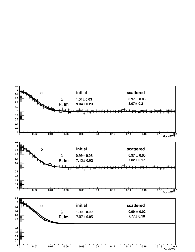
To test the UKM-R algorithm, we have implemented the above spherically symmetric Gaussian initial conditions and simulated the kinetic evolution in a number of events with fixed boson multiplicity $N=400$, choosing $T_{0}=0.130$ GeV and $R_{0}=7$ fm. To guarantee the nonrelativistic particle momenta, we have put $m=0.938$ GeV/c². The initial momentum and coordinate distributions are shown in Fig. 1. We have done two sets of simulations with the elastic cross sections $\sigma_{el}=$ $40$ and $400~{}$mb, assuming the isotropic scattering in the two-particle c.m. system. We have checked that the final results remain unchanged when introducing the cross section anisotropy.

Instead of the six-dimensional CF in Eq. (6), we have calculated one-dimensional ones integrating in numerator and denominator over all kinematic variables except a chosen one, e.g., the modulus ${\rm q}=|\mathbf{q}|$ of the relative momentum vector or its projections, or, the invariant relative momentum $q_{inv}=(\mathbf{q}^{2}-q_{0}^{2})^{1/2}=\mathrm{q}(1-v_{q}^{2})^{1/2}$, where $v_{q}$ is the projection of the pair velocity vector on the $\mathbf{q}$-direction; for nonrelativistic particles $v_{q}^{2}\ll 1$ and $q_{inv}\doteq{\rm q}$. As usual, we have assumed sufficiently smooth behaviour of the single-particle momentum spectrum (i.e., in our case, the initial thermal radius $R_{\mbox{\scriptsize th}}$ much smaller than the initial system radius $R_{0}$) and substituted the quasiaverages in Eq. (8) by the averages making the respective substitutions $x_{i},p\to x_{i},p_{i}$ and $\bar{x}_{i},p\to\bar{x}_{i},p_{i}$ in the arguments of the distribution and emission functions in the numerators. Explicit calculation at $t=0$ then leads to the Gaussian CF in Eq. (20) with the substitution $R_{0}^{2}-R_{\mbox{\scriptsize th}}^{2}\to R_{0}^{2}$. It should be noted however that this approximation violates the invariance of the four-vector product $qx$ on the trajectory of a free streaming particle (the invariance is guaranteed only for free streeming particle with the off-mass-shell four-momentum $p=(p_{1}+p_{2})/2$). As a result, the averages with distribution and emission functions are no more equivalent, the latter being preferable since it avoids free streaming from the emission or collision point to a given hypersurface $\sigma$.

Concerning the approximate averaging using the distribution function, at large evolution times $t$ as compared with the the mean emission time $\langle\bar{t}\rangle$, it leads to the additional oscillating factor in the CF,

$${\cal R}(t;\mathbf{p}_{1},\mathbf{p}_{2})\doteq 1+\exp\left(-R_{0}^{2}\mathbf{q}^{2}\right)\cos\left(\frac{t}{m}q_{inv}^{2}\right).$$ (22)

The oscillating factor invalidates the smoothness approximation at very large times and, at moderate times, it leads to an increase of the correlation radius, roughly,

$$R_{0}^{2}\to R_{0}^{2}+\left(\frac{kt}{mR_{0}}\right)^{2},$$ (23)

where the factor $k\sim 1$. For heavy particles of mass $m=0.938$ GeV/c² and the initial system radius $R_{0}=7$ fm, this increase does not exceed $10\%$ provided $t<100$ fm/c.

Similarly, the approximate averaging using the emission function at a current evolution time $t$ yields

$${\cal R}(t;\mathbf{p}_{1},\mathbf{p}_{2})\doteq 1+\exp\left(-R_{0}^{2}\mathbf{q}^{2}\right)\left\langle\cos\left(\frac{\bar{t}_{12}}{m}q_{inv}^{2}\right)\right\rangle_{\bar{t}_{1,2}\leq t},$$ (24)

where $\bar{t}_{12}=(\bar{t}_{1}+\bar{t}_{2})/2$ and the averaging is done over the emission times $\bar{t}_{1,2}\leq t$. For large evolution times, $t\sim t_{\mbox{\scriptsize out}}$, the distortion factor in Eq. (24) is independent of $t$ and its effect on the CF is determined by $\langle\bar{t}_{12}\rangle\ll t_{\mbox{\scriptsize out}}$. It thus leads to only a slight increase of the correlation radius, roughly determined by Eq. (23) with the substitution $t\to\langle\bar{t}_{12}\rangle$.

Practically, we have calculated the one–dimensional CF in the bins of a chosen variable $q_{j}$ (e.g., $q_{inv}$) as

$${\cal R}(q_{j})=\frac{1}{\Delta N(q_{j})}\sum_{i=1}^{\Delta N(q_{j})}[1+\cos(q^{(i)}x_{12}^{(i)})],$$ (25)

where $\Delta N(q_{j})$ is the number of simulated pairs in a given bin, consisting of the particles from the same event only; i.e., each pair from the same event was attributed the weight $[1+\cos(q^{(i)}x_{12}^{(i)})]$ and the weighted histogram of $q_{j}$ was produced. To determine the corresponding interferometry radius $R_{j}$, the constructed CF has been fitted as

$${\cal R}(q_{j})=1+\lambda\exp(-R_{j}^{2}q_{j}^{2}).$$ (26)

To check the exact solutions for the momentum and coordinate distributions in Eqs. (19) and (21) and the CF in Eq. (20), the particle coordinates and momenta have been evaluated at the following values of the evolution time $t$: 0, 50 and 100 fm/c. In Fig. 1 we show the results of the UKM-R simulations corresponding to the elastic cross section $\sigma_{el}=400$ mb; we have checked that they coincide with those obtained for $\sigma_{el}=40$ mb. These results confirm the independence of the momentum spectrum and the CF on the evolution time despite that a huge number of collisions happened during the evolution. A slight increase of the fitted interferometry radius at $t=100$ fm/c is a consequence of the smoothness approximation and agrees with Eqs. (22) and (23). As for the coordinate distribution, panel b of Fig. 1 confirms the increase of the system Gaussian radius with the evolution time in accordance with the law $R^{2}(t)=R_{0}^{2}+t^{2}T_{0}/m$. The results shown in Fig. 1 are in full correspondence with the exact solution of the BE for distribution function and thus confirm the correctness of the kinetic simulation.

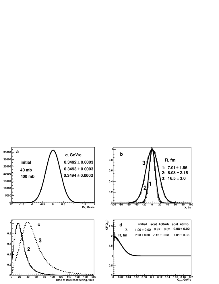
As noted after Eq. (22), the use of the smoothness approximation in the calculation of the CF with the help of the distribution function is invalidated at large evolution times. This is demonstrated in Fig. 2, where the appearance of the artificial zero of ${\cal R}(q_{inv})-1$ at $q_{inv}=(\pi m/2t)^{1/2}\approx 0.02$ GeV/c due to the oscillating factor in Eq. (22) is clearly seen in the CF calculated from boson coordinates at the evolution time $t=700$ fm/c. To calculate the correct CF at asymptotic times, we have therefore followed the system evolution up to a sufficiently large time ($t\sim 200$ fm/c for $\sigma_{el}=400$ mb) and taken as the particle four-coordinates those of the last emission or collision points. This corresponds to the system description with the help of the asymptotic emission function $S(x,p)$ which is much less affected by the smoothness approximation as compared with the distribution function. The spatial and time distributions of these points, corresponding to $\sigma_{el}=40$ and 400 mb, are shown in the panels ${\bf b}$ and ${\bf c}$ of Fig. 3. For $\sigma_{el}=40$ mb, one may see only a slight broadening of the spatial distribution as compared with the initial one and a quite narrow time distribution with a noticeable number of nonscattered particles ($t=0$) and the asymptotic time of $\sim 100$ fm/c. For $\sigma_{el}=400$ mb, the spatial and time distributions are much broader, almost all particles scatter at least once and the asymptotic time is $\sim 200$ fm/c. As for the asymptotic momentum spectra and interferometry radii, one may see from the panels ${\bf a}$ and ${\bf d}$ of Fig. 3 that they coincide with the initial ones within the errors for both values of $\sigma_{el}$.

VII Anisotropic, non-Gaussian and relativistic systems.

We have also studied to what extent are the spectra and CF’s conserved in kinetic evolution of nonrelativistic and relativistic systems characterized by initial conditions different from the spherically symmetric Gaussian ones given in Eq. (16) at $t=0$.

VII.1 Nonrelativistic systems.

VII.1.1 Anisotropic non-Gaussian spatial distribution.

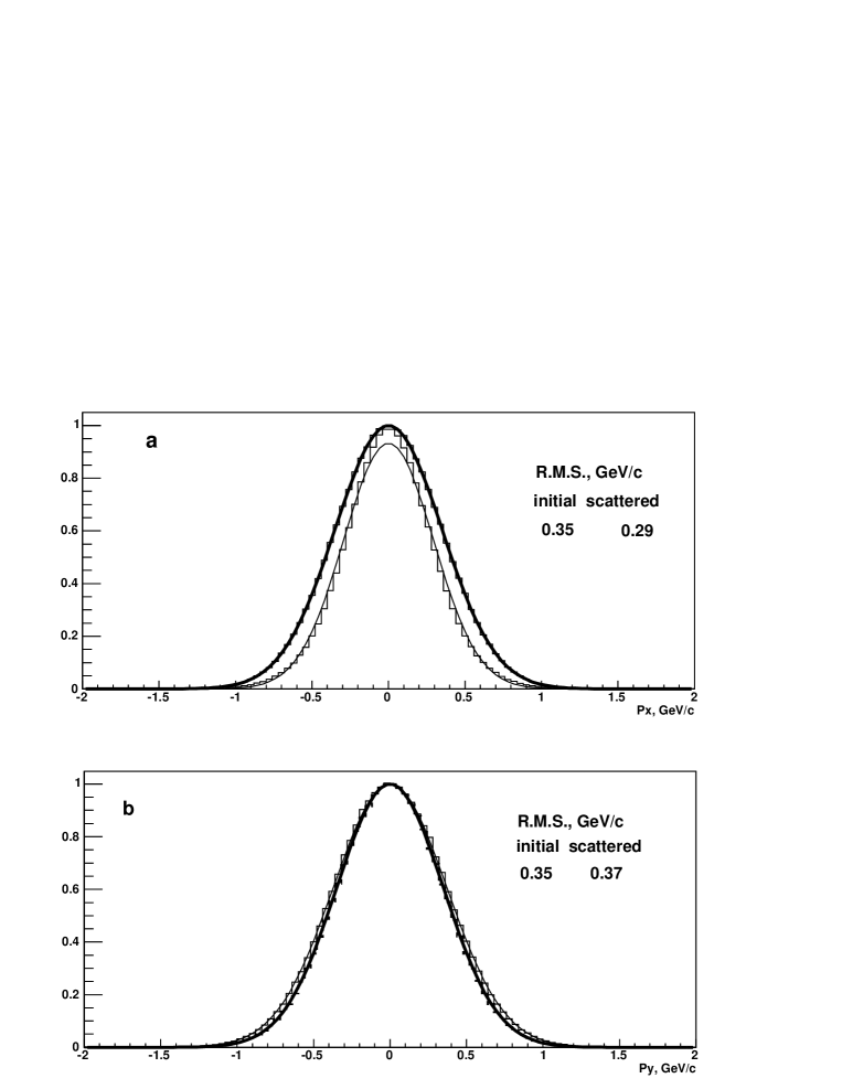
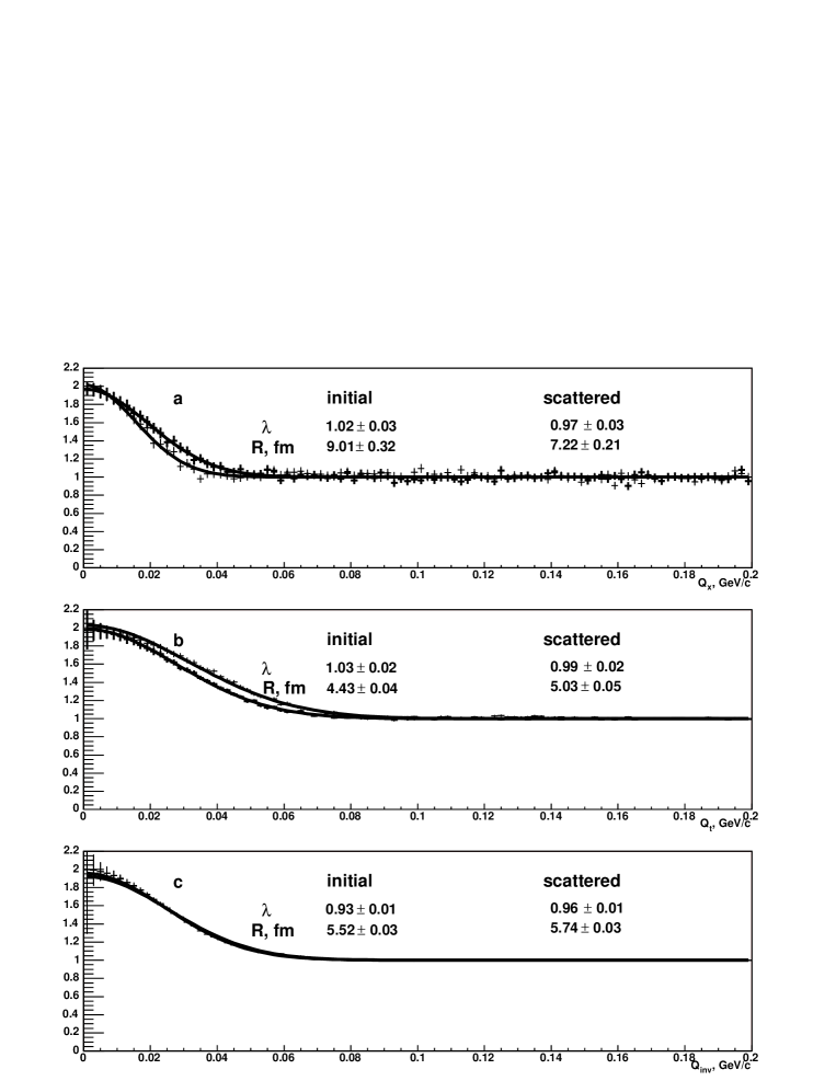
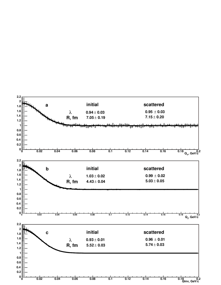
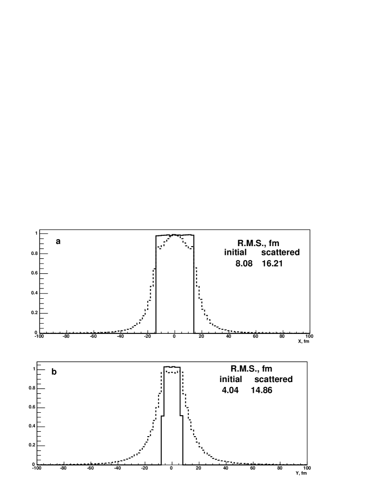
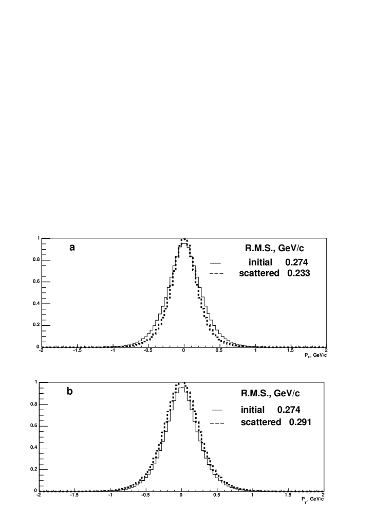
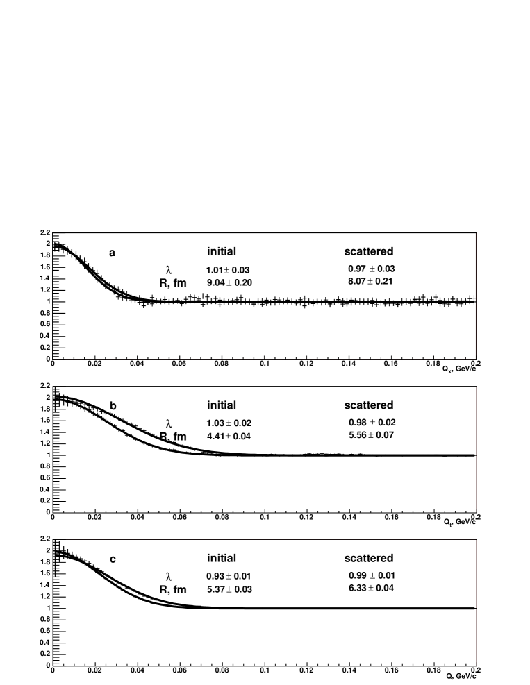
As in section VI, we have considered the nonrelativistic system of $N=400$ heavy spin-0 bosons of mass $m=0.938$ GeV/c² and the initial momentum distribution given in Eq. (19) with $T_{0}=0.130$ GeV. However, the initial spherically symmetric Gaussian spatial distribution was substituted by a uniformly populated parallelepiped defined by $|x|\leq 14$ fm and $|y|,|z|\leq 7$ fm (Fig. 4); the corresponding initial volume is about twice as large than in the previous case. The kinetic evolution was performed with two values of the elastic cross section, $\sigma_{el}=$ $40$ and $400~{}$mb. In the former case, the collisions are quite rare so the original spatial and momentum distributions, as well as the CF, are practically not changed during the evolution. In the latter case, the collisions are much more frequent and force the spatial distribution of the emission or last collision points to become close to a spherically symmetric Gaussian one (see dashed histograms in panels a and c of Fig. 4). On the other hand, as shown in Fig. 5, the initial space anisotropy is transformed in the anisotropy of the final three-momentum distribution. As compared with the originally spherically symmetric three-momentum distribution, the final one becomes softer in the $x$-direction and harder in the $(y,z)$-plane. As for the CF’s, one may see from Fig. 6 that their evolution reflects the one of the emission points, the final CF’s becoming closer to spherical symmetry. It is interesting to note that despite of the noticeable difference of the initial and final CF’s, the interferometry volume, $R_{x}R_{t}^{2}$, is practically not changed during the evolution, the initial and final one composing $177\pm 6$ and $182\pm 6$ fm³ respectively. Also the $q_{inv}$ projection of the CF is changed only slightly (see panel c in Fig. 4). The effect of approximate conservation of the interferometry volume is in correspondence with a similar result found for the chemically frozen hydrodynamic evolution akksin .

VII.1.2 Nonthermal momentum distribution

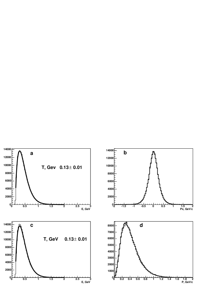
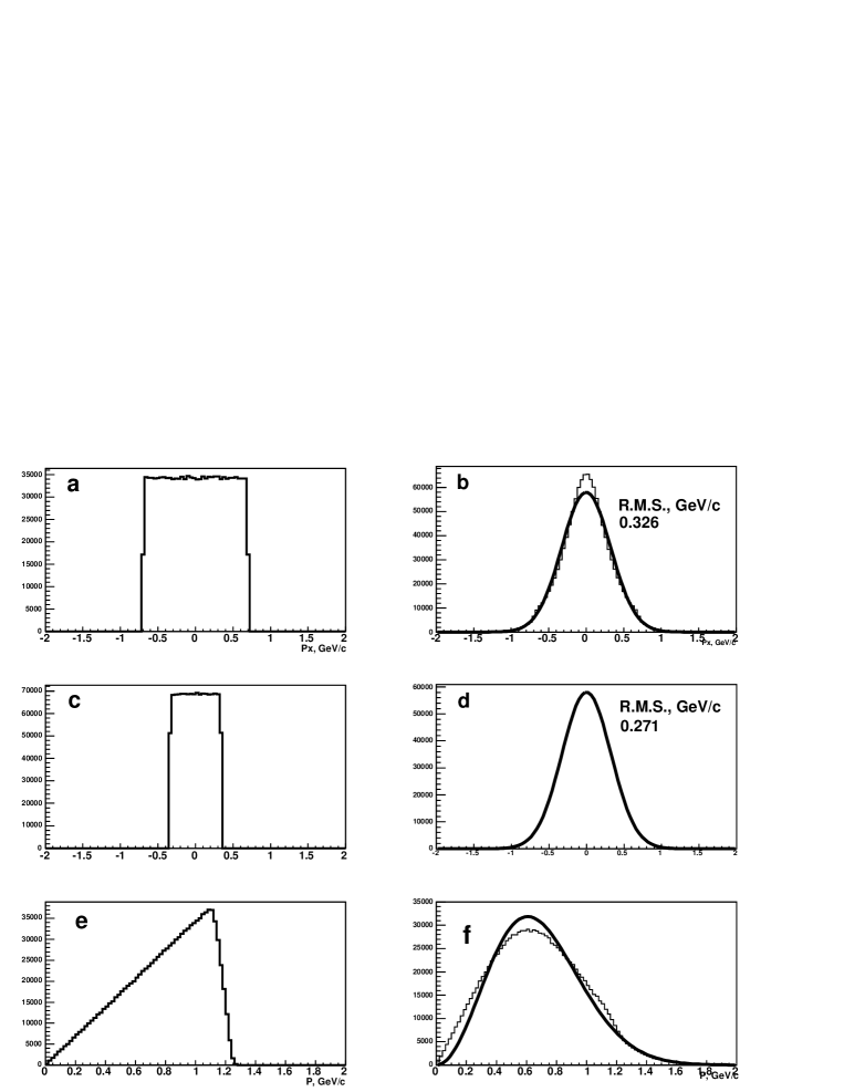
We have further considered the same initial conditions as in section VI except for the thermal Gaussian three–momentum distribution which has been substituted by a uniformly populated cube defined by $|p_{x}|,|p_{y}|,|p_{z}|\leq(T_{0}m)^{1/2}$, $T_{0}$ = 0.130 GeV, $m=$0.938 GeV/c² (Fig. 7). The results of the kinetic evolution of the momentum distribution and the CF’s corresponding to the initial Gaussian radius $R_{0}=7$ fm and the elastic cross section $\sigma_{el}=400$ mb are shown in figures 7 and 8; similar results have been obtained with $\sigma_{el}=40$ mb. One may see that the collisions force the initially nonthermal distribution to take the thermal Gaussian form. At the same time, r.m.s. of the initial distribution of the momentum components, $\sigma=(mT_{0}/3)^{1/2}=201.6$ MeV/c, as well as the initial CF and the interferometry radius of 7 fm, are practically conserved. E.g., the Gaussian fits of the $p_{x}$ distribution and the $q_{t}$ projection of the CF yield $\sigma=202.4\pm 0.2$ MeV/c and $R_{t}=7.14\pm 0.11$ fm respectively.

VII.2 Relativistic systems.

We have also studied the kinetic evolution of the relativistic hadronic gas ($m\sim T_{0}$) choosing the particle mass $m=0.140$  GeV/c² and the initial temperature $T_{0}=0.130$ GeV. It is well known that the only relativistic solution of the BE with vanishing collision term is the $x$-independent Jüttner distribution function,

$$f(x,p)=\frac{1}{(2\pi)^{3}}\exp\left(\frac{\mu-p^{\mu}U_{\mu}}{T}\right),$$ (27)

corresponding to a global thermal equilibrium with temperature $T$, chemical potential $\mu$ and system four-velocity $U$. Particularly, the relativistic generalization of the distribution function in Eq. (16),

$$f(x,p)\propto\exp\left(-\frac{(\mathbf{r}-t\mathbf{p}/p^{0})^{2}}{2R_{0}^{2}}-\frac{p^{0}}{T_{0}}\right),$$ (28)

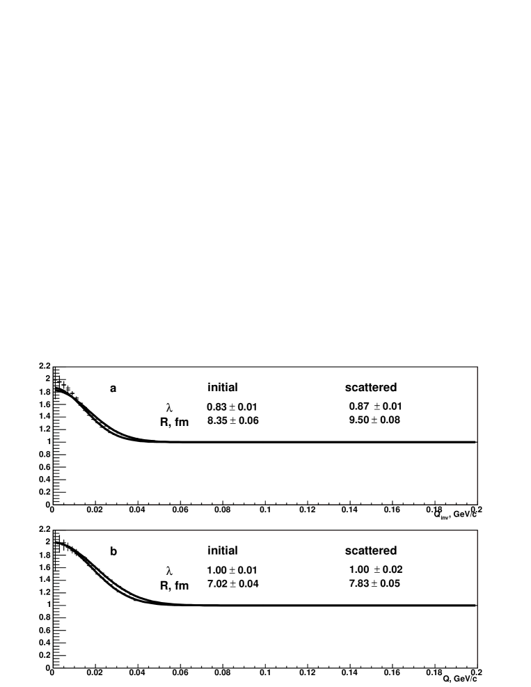
represents only an approximate solution of the BE, leading to vanishing l.h.s. but retaining a nonzero r.h.s. collision term. Generally, one may expect that, irrespective of initial conditions, the distribution function formed in the kinetic evolution should tend to the Jüttner one, i.e., the spatial distribution should expand and the three–momentum distribution $d^{3}N/d^{3}{\bf p}$ should tend to the thermal one $\propto\exp[-({\bf p}^{2}+m^{2})^{1/2}/T]$. Particularly, starting the kinetic evolution from the initial conditions corresponding to Eq. (28) at $t=0$, one may expect an increase of the system Gaussian radius with the evolution time and conserved momentum distribution. Based on the analogy with the nonrelativistic system, one can also expect an approximate conservation of the correlation radius. To check these expectations, we have put the initial Gaussian radius $R_{0}=7$ fm and simulated the kinetic evolution for $N=400$ particles with the elastic cross section $\sigma_{el}=400$ mb. The simulation results shown in figures 9 and  10 indeed confirm the conservation of the momentum spectrum and approximate conservation of the CF, the final correlation radius exceeding the initial one by $\sim 9\%$ only. We have obtained the same results for $N=40000$ particles and $\sigma_{el}=4$ mb thus proving the negligible effect of the violation of Lorentz covariance introduced by the nonlocal condition in Eq. (14); some deviations start to appear only at $\sigma_{el}\sim 1000$ mb.

VII.2.1 Anisotropic non-Gaussian spatial distribution.

We have considered the same initial anisotropic coordinate distributions as for the nonrelativistic bosons. Comparing figures 4-6 and 11-13 corresponding respectively to nonrelativistic and relativistic bosons, one observes similar isotropisation effects in the distributions of the emission points and CF’s, as well as similar anisotropy transfer from spatial to momentum components of the phase space emission points. The interferometry volume is however conserved only approximately, it increases by $\sim 30\%$ from the initial value of $\sim 176~{}$ fm³ to the final one of $\sim$ 250  fm³.

VII.2.2 Nonthermal anisotropic momentum distribution

We have further considered the same initial conditions as in Fig. 9 except for the thermal momentum distribution which has been substituted by a uniformly populated parallelepiped defined by $|p_{x}|\leq 0.7$ GeV/c, $|p_{y}|,|p_{z}|\leq 0.35$ GeV (Fig. 14). The results of the kinetic evolution of the three-momentum distribution and the CF’s are shown in figures 14 and 15. One may see that the collisions force the initially nonthermal distribution to become close to the thermal one. The final interferometry radii are $\sim 10\%$ higher than the initial one of 7 fm, similar to the case of the initial thermal momentum distribution.

VIII Conclusions and outlook

We have studied numerical solutions of the Boltzmann equation in the Universal Kinetic Model. First, we have tested the model kinetic algorithm recovering the known nonrelativistic solution [1-3] for the spherically symmetric Gaussian initial conditions up to the elastic cross section of 1000 mb. Particularly, we have checked that despite a huge number of collisions the momentum spectra and interferometry radii remain unchanged during the evolution. Further, we have modified the initial conditions and found that with the increasing elastic cross section the system of nonrelativistic particles more and more recovers spherical symmetry and thermal momentum distribution. At the same time, similar to the above case, the momentum dispersion and the interferometry volume is practically conserved during the evolution. The conservation effect takes place also in the evolution of the system of relativistic particles, except for some increase ($\sim 30\%$ at 400 mb) of the final interferometry volume. Our studies thus support similar results obtained in hydrodynamic approximation in Ref. akksin .

It is worth to note that the initially anisotropic system tends to an isotropic one and, after sufficiently large number of collisions, the spectra and interferometry radii are approximately conserved in subsequent evolution. In such a case one can exploit the idea of duality of hydrodynamic and kinetic descriptions of interferometry volumes and effective temperatures (momentum dispersions) Borysova , i.e. estimate their values from the thermal hadronic distribution function in the initially formed hadronic fireball instead of a detailed analysis based on the complicated asymptotic distribution or emission functions.

We plan to extend the analysis of kinetic evolution of the spectra and interferometry radii to many component hadron gases, including inelastic collisions and resonance decays.

Figure 1: Distributions of the $x$-components of particle three-momentum (a) and three-coordinate (b), particle momentum (c) and the corresponding CF’s as functions of $q_{inv}$ (d) obtained in the UKM-R simulation of the kinetic evolution of $N=400$ heavy spin-0 bosons of mass $m=0.938$ GeV/c² at the evolution time $t=0$, 50 and 100 fm/c. The elastic cross section $\sigma_{el}=400$ mb, the initial Gaussian radius $R_{0}=7$ fm and the initial temperature $T_{0}=0.130$ GeV. The shown results of Gaussian fits of the momentum distributions and the CF’s agree with the input initial values $\sigma=(mT_{0})^{1/2}=0.3492$ GeV/c and $\lambda=1$, $R_{0}=7$ fm respectively.

Figure 2: CF’s obtained from four-coordinates of free streaming ($\sigma_{el}=0$) heavy spin-0 bosons of mass $m=0.938$ GeV/c² obtained in the UKM-R simulation on the same conditions as in Fig. 1 at the evolution times $100$ and 700 fm/c.

Figure 3: Initial and final distributions of the $x$-components of particle three-momentum (a), spatial $x$- (b) and time (c) coordinates of the emission or last collision points and the CF’s corresponding to these points as functions of $q_{inv}$ (d) obtained in the UKM-R simulation of $N=400$ heavy spin-0 bosons of mass $m=0.938$ GeV/c² at the evolution time $t=$ 200 fm/c. The histograms 1, 2 and 3 in panels b and c correspond to $\sigma_{el}=$ 0 (initial $x$-distribution), 40 and 400 mb respectively. The shown results of Gaussian fits of the momentum distributions and the CF’s agree with the input initial values $\sigma=(mT_{0})^{1/2}=0.3492$ GeV/c and $\lambda=1$, $R_{0}=7$ fm respectively.

Figure 4: Final distributions of $x$- and $y$-coordinates of the emission or last collision points (dashed histograms) obtained in the UKM-R simulation on the same conditions as in Fig. 3 except for the initial distributions of spatial coordinates (solid histograms): $|x|\leq 14$ Fm, $|y|,|z|\leq 7$ Fm. The panels a, c and b, d correspond to $\sigma_{el}=$ 400 and 40 mb respectively.

Figure 5: Initial (thick) and final (thin) histograms of the components of particle three–momentum obtained in the UKM-R simulation on the same conditions as in Fig. 4.

Figure 6: Initial and final CF’s corresponding to the UKM-R coordinate distributions in panels a and c of Fig. 4 ($\sigma_{el}=400$ mb). The CF’s are shown as functions of $q_{x}$ ($q_{t}\leq 10$ MeV/c) (a), $q_{t}=({q_{y}}^{2}+{q_{z}}^{2})^{1/2}$ ($q_{x}\leq 7$ MeV/c) (b) and $q_{inv}$ (c). The results of Gaussian fits are shown. The fitted initial Gaussian radii in panels a and b are close to the r.m.s. values 8.08 and 4.04 fm of the corresponding initial $x$- and $y$-coordinate distributions in panels a and c of Fig. 4.

Figure 7: Final distributions of the $x$-component (b) and the magnitude of particle three–momentum (d) obtained in the UKM-R simulation with $\sigma_{el}=$ 400 mb on the same conditions as in Fig. 3 except for the initial three–momentum distribution (a and c) defined by $|p_{x}|,|p_{y}|,|p_{z}|\leq(T_{0}m)^{1/2}$, $T_{0}$ = 0.130 GeV, $m=$0.938 GeV/c². The fitted Gaussian widths of final distributions, shown in panels b and d, are close to the r.m.s. value $(mT_{0}/3)^{1/2}$ = 0.2016 GeV of the initial $p_{x}$-distribution.

Figure 8: Initial and final CF’s corresponding to the UKM-R simulation specified in the caption of Fig. 7. The CF’s are shown as functions of $q_{x}$ ($q_{t}\leq 10$ MeV/c) (a), $q_{t}=({q_{y}}^{2}+{q_{z}}^{2})^{1/2}$ ($q_{x}\leq 7$ MeV/c) (b) and $q_{inv}$ (c). The results of Gaussian fits are shown. The fitted correlation radii are close to the initial system Gaussian radius $R_{0}=7$ fm.

Figure 9: Distributions of particle energy (a, c), momentum (d) and $x$-component of particle three-momentum (b) obtained in the UKM-R simulation of the kinetic evolution of $N=400$ light spin-0 bosons of mass $m=0.140$ GeV/c² and elastic cross section $400$ mb. The initial three–coordinates and three–momenta have been respectively distributed according to Gaussian of the radius $R_{0}=7$ fm and relativistic thermal distribution with the temperature $T_{0}=0.130$ GeV. The initial distributions are shown as solid histograms in panels a, b, d and the final ones - as solid histogram in panel c and dashed histograms in panels b, d. The fitted values of the initial and final temperature shown in panels a and c coincide with $T_{0}$.

Figure 10: Initial and final CF’s corresponding to the UKM-R simulation specified in the caption of Fig. 9. The CF’s are shown as functions of $q_{inv}$ (a) and ${\rm q}=|{\bf q}|$ (b).

Figure 11: Final distributions of $x$- (a) and $y$- (b) coordinates of the emission or last collision points (dashed histograms) obtained in the UKM-R simulation on the same conditions as in Fig. 9 except for the initial distributions of spatial coordinates (solid histograms): $|x|\leq 14$ Fm, $|y|,|z|\leq 7$ Fm.

Figure 12: Initial (solid) and final (dashed) histograms of the components of particle three–momentum obtained in the UKM-R simulation on the same conditions as in Fig. 11.

Figure 13: Initial and final CF’s corresponding to the UKM-R simulation specified in the caption of Fig. 11. The CF’s are shown as functions of $q_{x}$ ($q_{t}\leq 10$ MeV/c), $q_{t}=({q_{y}}^{2}+{q_{z}}^{2})^{1/2}$ ($q_{x}\leq 7$ MeV/c) and ${\rm q}=|{\bf q}|$.

Figure 14: Final distributions of the components (b, d) and the magnitude (f) of particle three–momentum obtained in the UKM-R simulation with $\sigma_{el}=$ 400 mb on the same conditions as in Fig. 9 except for the initial three–momentum distribution (a, c, e) defined by $|p_{x}|\leq 0.7$ GeV/c, $|p_{y}|,|p_{z}|\leq 0.35$ GeV/c. The fitted Gaussian widths of final distributions are shown in panels b, d and f.

Figure 15: Initial and final CF’s corresponding to the UKM-R simulation specified in the caption of Fig. 14. The CF’s are shown as functions of $q_{x}$ ($q_{t}\leq 10$ MeV/c), $q_{t}=({q_{y}}^{2}+{q_{z}}^{2})^{1/2}$ ($q_{x}\leq 7$ MeV/c) and ${\rm q}=|{\bf q}|$.