Exact Analytical Solution of the Constrained Statistical Multifragmentation Model and Phase Transitions in Finite Systems

Abstract

We discuss an exact analytical solution of a simplified version of the statistical multifragmentation model with the restriction that the largest fragment size cannot exceed the finite volume of the system. A complete analysis of the isobaric partition singularities of this model is done for finite volumes. It is shown that the real part of any simple pole of the isobaric partition defines the free energy of the corresponding state, whereas its imaginary part, depending on the sign, defines the inverse decay/formation time of this state. The developed formalism allows us, for the first time, to exactly define the finite volume analogs of gaseous, liquid and mixed phases of this model from the first principles of statistical mechanics and demonstrate the pitfalls of earlier works. The finite size effects for large fragments and the role of metastable (unstable) states are discussed.

PACS numbers: 25.70. Pq, 21.65.+f, 24.10. Pa

I Introduction

A great deal of progress was recently achieved in our understanding of the multifragmentation phenomenon Bondorf:95 ; Gross:97 ; Moretto:97 when an exact analytical solution of a simplified version of the statistical multifragmentation model (SMM) Gupta:98 ; Gupta:99 was found in Refs. Bugaev:00 ; Bugaev:01 ; Reuter:01 . An invention of a new powerful mathematical method Bugaev:04a , the Laplace-Fourier transform, allowed us not only to solve this version of SMM analytically for finite volumes Bugaev:04a , but to find the surface partition and surface entropy of large clusters for a variety of statistical ensembles Bugaev:04b . It was shown Bugaev:04a that for finite volumes the analysis of the grand canonical partition (GCP) of the simplified SMM is reduced to the analysis of the simple poles of the corresponding isobaric partition, obtained as a Laplace-Fourier transform of the GCP. This method opens a principally new possibility to study the nuclear liquid-gas phase transition directly from the partition of finite system and without taking its thermodynamic limit.

Exactly solvable models with phase transitions play a special role in the statistical physics - they are the benchmarks of our understanding of critical phenomena that occur in more complicated substances. They are our theoretical laboratories, where we can study the most fundamental problems of critical phenomena which cannot be studied elsewhere. Note that these questions in principle cannot be clarified either within the widely used mean-filed approach or numerically.

Despite this success, the application of the exact solution Bugaev:00 ; Bugaev:01 ; Reuter:01 to the description of experimental data is limited because this solution corresponds to an infinite system volume. Therefore, from a practical point of view it is necessary to extend the formalism for finite volumes. Such an extension is also necessary because, despite a general success in the understanding the nuclear multifragmentation, there is a lack of a systematic and rigorous theoretical approach to study the phase transition phenomena in finite systems. For instance, even the best formulation of the statistical mechanics and thermodynamics of finite systems by Hill Hill is not rigorous while discussing the phase transitions. Exactly solvable models of phase transitions applied to finite systems may provide us with the first principle results unspoiled by the additional simplifying assumptions. Here we present a finite volume extension of the SMM.

To have a more realistic model for finite volumes, we would like to account for the finite size and geometrical shape of the largest fragments, when they are comparable with the system volume. For this we will abandon the arbitrary size of largest fragment and consider the constrained SMM (CSMM) in which the largest fragment size is explicitly related to the volume $V$ of the system. A similar model, but with the fixed size of the largest fragment, was recently analyzed in Ref. CSMM .

In this work we will: solve the CSMM analytically at finite volumes using a new powerful method; consider how the first order phase transition develops from the singularities of the SMM isobaric partition Goren:81 in thermodynamic limit; study the finite volume analogs of phases; and discuss the finite size effects for large fragments.

II Laplace-Fourier Transformation

The system states in the SMM are specified by the multiplicity sets $\{n_{k}\}$ ($n_{k}=0,1,2,...$) of $k$-nucleon fragments. The partition function of a single fragment with $k$ nucleons is Bondorf:95 : $V\phi_{k}(T)=V\left(mTk/2\pi\right)^{3/2}~{}z_{k}~{}$, where $k=1,2,...,A$ ($A$ is the total number of nucleons in the system), $V$ and $T$ are, respectively, the volume and the temperature of the system, $m$ is the nucleon mass. The first two factors on the right hand side (r.h.s.) of the single fragment partition originate from the non-relativistic thermal motion and the last factor, $z_{k}$, represents the intrinsic partition function of the $k$-nucleon fragment. Therefore, the function $\phi_{k}(T)$ is a phase space density of the k-nucleon fragment. For $k=1$ (nucleon) we take $z_{1}=4$ (4 internal spin-isospin states) and for fragments with $k>1$ we use the expression motivated by the liquid drop model (see details in Ref. Bondorf:95 ): $z_{k}=\exp(-f_{k}/T),$ with fragment free energy

$$f_{k}=-W(T)~{}k+\sigma(T)~{}k^{2/3}+(\tau+3/2)T\ln k~{},$$ (1)

with $W(T)=W_{\rm o}+T^{2}/\epsilon_{\rm o}$. Here $W_{\rm o}=16$ MeV is the bulk binding energy per nucleon. $T^{2}/\epsilon_{\rm o}$ is the contribution of the excited states taken in the Fermi-gas approximation ($\epsilon_{\rm o}=16$ MeV). $\sigma(T)$ is the temperature dependent surface tension parameterized in the following relation: $\sigma(T)=\sigma_{\rm o}[(T_{c}^{2}~{}-~{}T^{2})/(T_{c}^{2}~{}+~{}T^{2})]^{5/4},$ with $\sigma_{\rm o}=18$ MeV and $T_{c}=18$ MeV ($\sigma=0$ at $T\geq T_{c}$). The last contribution in Eq. (1) involves the famous Fisher’s term with dimensionless parameter $\tau$.

The canonical partition function (CPF) of nuclear fragments in the SMM has the following form:

$$Z^{id}_{A}(V,T)=\sum_{\{n_{k}\}}\biggl{[}\prod_{k=1}^{A}\frac{\left[V~{}\phi_{k}(T)\right]^{n_{k}}}{n_{k}!}\biggr{]}{\textstyle\delta(A-\sum_{k}kn_{k})}\,.$$ (2)

In Eq. (2) the nuclear fragments are treated as point-like objects. However, these fragments have non-zero proper volumes and they should not overlap in the coordinate space. In the excluded volume (Van der Waals) approximation this is achieved by substituting the total volume $V$ in Eq. (2) by the free (available) volume $V_{f}\equiv V-b\sum_{k}kn_{k}$, where $b=1/\rho_{{\rm o}}$ ($\rho_{{\rm o}}=0.16$ fm^-3 is the normal nuclear density). Therefore, the corrected CPF becomes: $Z_{A}(V,T)=Z^{id}_{A}(V-bA,T)$. The SMM defined by Eq. (2) was studied numerically in Refs. Gupta:98 ; Gupta:99 . This is a simplified version of the SMM, e.g. the symmetry and Coulomb contributions are neglected. However, its investigation appears to be of principal importance for studies of the liquid-gas phase transition.

The calculation of $Z_{A}(V,T)$ is difficult due to the constraint $\sum_{k}kn_{k}=A$. This difficulty can be partly avoided by evaluating the grand canonical partition (GCP)

$${\cal Z}(V,T,\mu)~{}\equiv~{}\sum_{A=0}^{\infty}\exp\left({\textstyle\frac{\mu A}{T}}\right)Z_{A}(V,T)~{}\Theta(V-bA)~{},$$ (3)

where $\mu$ denotes a chemical potential. The calculation of ${\cal Z}$ is still rather difficult. The summation over $\{n_{k}\}$ sets in $Z_{A}$ cannot be performed analytically because of additional $A$-dependence in the free volume $V_{f}$ and the restriction $V_{f}>0$. This problem was resolved Bugaev:00 ; Bugaev:01 by the Laplace transformation method to the so-called isobaric ensemble Goren:81 .

In this work we would like to consider a more strict constraint $\sum\limits_{k}^{K(V)}k~{}n_{k}=A$ , where the size of the largest fragment $K(V)=\alpha V/b$ cannot exceed the total volume of the system (the parameter $\alpha\leq 1$ is introduced for convenience). The case $K(V)=Const$ is also included in our treatment. A similar restriction should be also applied to the upper limit of the product in all partitions $Z_{A}^{id}(V,T)$, $Z_{A}(V,T)$ and ${\cal Z}(V,T,\mu)$ introduced above (how to deal with the real values of $K(V)$, see later). Then the model with this constraint, the CSMM, cannot be solved by the Laplace transform method, because the volume integrals cannot be evaluated due to a complicated functional $V$-dependence. However, the CSMM can be solved analytically with the help of the following identity

$$G(V)=\int\limits_{-\infty}^{+\infty}d\xi~{}\int\limits_{-\infty}^{+\infty}\frac{d\eta}{{2\pi}}~{}{\textstyle e^{i\eta(V-\xi)}}~{}G(\xi)\,,$$ (4)

which is based on the Fourier representation of the Dirac $\delta$-function. The representation (4) allows us to decouple the additional volume dependence and reduce it to the exponential one, which can be dealt by the usual Laplace transformation in the following sequence of steps

$$\hat{\cal Z}(\lambda,T,\mu)~{}\equiv~{}\int_{0}^{\infty}dV~{}{\textstyle e^{-\lambda V}}~{}{\cal Z}(V,T,\mu)=$$

$$\int_{0}^{\infty}dV^{\prime}\int\limits_{-\infty}^{+\infty}d\xi~{}\int\limits_{-\infty}^{+\infty}\frac{d\eta}{{2\pi}}~{}{\textstyle e^{i\eta(V^{\prime}-\xi)-\lambda V^{\prime}}}\times$$

$$\sum_{\{n_{k}\}}\left[\prod_{k=1}^{K(\xi)}~{}\frac{1}{n_{k}!}~{}\left\{V^{\prime}~{}{\textstyle\phi_{k}(T)\,e^{\frac{(\mu-(\lambda-i\eta)bT)k}{T}}}\right\}^{n_{k}}\right]\Theta(V^{\prime})=$$

$$\int_{0}^{\infty}dV^{\prime}\int\limits_{-\infty}^{+\infty}d\xi~{}\int\limits_{-\infty}^{+\infty}\frac{d\eta}{{2\pi}}~{}{\textstyle e^{i\eta(V^{\prime}-\xi)-\lambda V^{\prime}+V^{\prime}{\cal F}(\xi,\lambda-i\eta)}}\,.$$ (5)

After changing the integration variable $V\rightarrow V^{\prime}=V-b\sum\limits_{k}^{K(\xi)}k~{}n_{k}$, the constraint of $\Theta$-function has disappeared. Then all $n_{k}$ were summed independently leading to the exponential function. Now the integration over $V^{\prime}$ in Eq. (II) can be straightforwardly done resulting in

$$\hat{\cal Z}(\lambda,T,\mu)=\int\limits_{-\infty}^{+\infty}d\xi\int\limits_{-\infty}^{+\infty}\frac{d\eta}{{2\pi}}~{}\frac{\textstyle e^{-i\eta\xi}}{{\textstyle\lambda-i\eta~{}-~{}{\cal F}(\xi,\lambda-i\eta)}}~{},$$ (6)

where the function ${\cal F}(\xi,\tilde{\lambda})$ is defined as follows

$${\cal F}(\xi,\tilde{\lambda})=\sum\limits_{k=1}^{K(\xi)}\phi_{k}(T)~{}e^{\frac{(\mu-\tilde{\lambda}bT)k}{T}}=$$

$$\left(\frac{mT}{2\pi}\right)^{\frac{3}{2}}\biggl{[}z_{1}~{}{\textstyle e^{\frac{\mu-\tilde{\lambda}bT}{T}}}+\sum_{k=2}^{K(\xi)}k^{-\tau}e^{\frac{(\mu+W-\tilde{\lambda}bT)k-\sigma k^{2/3}}{T}}\biggr{]}\,.\,$$ (7)

As usual, in order to find the GCP by the inverse Laplace transformation, it is necessary to study the structure of singularities of the isobaric partition (II).

III Isobaric Partition Singularities

The isobaric partition (II) of the CSMM is, of course, more complicated than its SMM analog Bugaev:00 ; Bugaev:01 because for finite volumes the structure of singularities in the CSMM is much richer than in the SMM, and they match in the limit $V\rightarrow\infty$ only. To see this let us first make the inverse Laplace transform:

$${\cal Z}(V,T,\mu)~{}=\int\limits_{\chi-i\infty}^{\chi+i\infty}\frac{d\lambda}{2\pi i}~{}\hat{\cal Z}(\lambda,T,\mu)~{}e^{\textstyle\lambda\,V}=$$

$$\int\limits_{-\infty}^{+\infty}d\xi\int\limits_{-\infty}^{+\infty}\frac{d\eta}{{2\pi}}\int\limits_{\chi-i\infty}^{\chi+i\infty}\frac{d\lambda}{2\pi i}~{}\frac{\textstyle e^{\lambda\,V-i\eta\xi}}{{\textstyle\lambda-i\eta~{}-~{}{\cal F}(\xi,\lambda-i\eta)}}~{}=$$

$$\int\limits_{-\infty}^{+\infty}d\xi\int\limits_{-\infty}^{+\infty}\frac{d\eta}{{2\pi}}\,{\textstyle e^{i\eta(V-\xi)}}\sum_{\{\lambda_{n}\}}e^{\textstyle\lambda_{n}\,V}{\textstyle\left[1-\frac{\partial{\cal F}(\xi,\lambda_{n})}{\partial\lambda_{n}}\right]^{-1}}\,,$$ (8)

where the contour $\lambda$-integral is reduced to the sum over the residues of all singular points $\lambda=\lambda_{n}+i\eta$ with $n=1,2,..$, since this contour in the complex $\lambda$-plane obeys the inequality $\chi>\max(Re\{\lambda_{n}\})$. Now both remaining integrations in (III) can be done, and the GCP becomes

$${\cal Z}(V,T,\mu)~{}=\sum_{\{\lambda_{n}\}}e^{\textstyle\lambda_{n}\,V}{\textstyle\left[1-\frac{\partial{\cal F}(V,\lambda_{n})}{\partial\lambda_{n}}\right]^{-1}}\,,$$ (9)

i.e. the double integral in (III) simply reduces to the substitution $\xi\rightarrow V$ in the sum over singularities. This is a remarkable result which can be formulated as the following theorem: if the Laplace-Fourier image of the excluded volume GCP exists, then for any additional $V$-dependence of ${\cal F}(V,\lambda_{n})$ or $\phi_{k}(T)$ the GCP can be identically represented by Eq. (9).

The simple poles in (III) are defined by the equation

$$\lambda_{n}~{}=~{}{\cal F}(V,\lambda_{n})\,.$$ (10)

In contrast to the usual SMM Bugaev:00 ; Bugaev:01 the singularities $\lambda_{n}$ are (i) are volume dependent functions, if $K(V)$ is not constant, and (ii) they can have a non-zero imaginary part, but in this case there exist pairs of complex conjugate roots of (10) because the GCP is real.

Introducing the real $R_{n}$ and imaginary $I_{n}$ parts of $\lambda_{n}=R_{n}+iI_{n}$, we can rewrite Eq. (10) as a system of coupled transcendental equations

$$R_{n}=~{}\sum\limits_{k=1}^{K(V)}\tilde{\phi}_{k}(T)~{}{\textstyle e^{\frac{Re(\nu_{n})\,k}{T}}}\cos(I_{n}bk)\,,$$ (11)

$$I_{n}=-\sum\limits_{k=1}^{K(V)}\tilde{\phi}_{k}(T)~{}{\textstyle e^{\frac{Re(\nu_{n})\,k}{T}}}\sin(I_{n}bk)\,,$$ (12)

where we have introduced the set of the effective chemical potentials $\nu_{n}\equiv\nu(\lambda_{n})$ with $\nu(\lambda)=\mu+W(T)-\lambda b\,T$, and the reduced distributions $\tilde{\phi}_{1}(T)=\left(\frac{mT}{2\pi}\right)^{\frac{3}{2}}z_{1}\exp(-W(T)/T)$ and $\tilde{\phi}_{k>1}(T)=\left(\frac{mT}{2\pi}\right)^{\frac{3}{2}}k^{-\tau}\,\exp(-\sigma(T)~{}k^{2/3}/T)$ for convenience.

Consider the real root $(R_{0}>0,I_{0}=0)$, first. For $I_{n}=I_{0}=0$ the real root $R_{0}$ exists for any $T$ and $\mu$. Comparing $R_{0}$ with the expression for vapor pressure of the analytical SMM solution Bugaev:00 ; Bugaev:01 shows that $TR_{0}$ is a constrained grand canonical pressure of the gas. As usual, for finite volumes the total mechanical pressure Hill , as we will see in section V, differs from $TR_{0}$. Equation (12) shows that for $I_{n>0}\neq 0$ the inequality $\cos(I_{n}bk)\leq 1$ never become the equality for all $k$-values simultaneously. Then from Eq. (11) one obtains ($n>0$)

$$R_{n}<\sum\limits_{k=1}^{K(V)}\tilde{\phi}_{k}(T)~{}{\textstyle e^{\frac{Re(\nu_{n})\,k}{T}}}\quad\Rightarrow\quad R_{n}<R_{0}\,,$$ (13)

where the second inequality (13) immediately follows from the first one. In other words, the gas singularity is always the rightmost one. This fact plays a decisive role in the thermodynamic limit $V\rightarrow\infty$.

The interpretation of the complex roots $\lambda_{n>0}$ is less straightforward. According to Eq. (9), the GCP is a superposition of the states of different free energies $-\lambda_{n}VT$. (Strictly speaking, $-\lambda_{n}VT$ has a meaning of the change of free energy, but we will use the traditional term for it.) For $n>0$ the free energies are complex. Therefore, $-\lambda_{n>0}T$ is the density of free energy. The real part of the free energy density, $-R_{n}T$, defines the significance of the state’s contribution to the partition: due to (13) the largest contribution always comes from the gaseous state and has the smallest real part of free energy density. As usual, the states which do not have the smallest value of the (real part of) free energy, i. e. $-R_{n>0}T$, are thermodynamically metastable. For infinite volume they should not contribute unless they are infinitesimally close to $-R_{0}T$, but for finite volumes their contribution to the GCP may be important.

As one sees from (11) and (12), the states of different free energies have different values of the effective chemical potential $\nu_{n}$, which is not the case for infinite volume Bugaev:00 ; Bugaev:01 , where there exists a single value for the effective chemical potential. Thus, for finite $V$ the states which contribute to the GCP (9) are not in a true chemical equilibrium.

The meaning of the imaginary part of the free energy density becomes clear from (11) and (12): as one can see from (11) the imaginary part $I_{n>0}$ effectively changes the number of degrees of freedom of each $k$-nucleon fragment ($k\leq K(V)$) contribution to the free energy density $-R_{n>0}T$. It is clear, that the change of the effective number of degrees of freedom can occur virtually only and, if $\lambda_{n>0}$ state is accompanied by some kind of equilibration process. Both of these statements become clear, if we recall that the statistical operator in statistical mechanics and the quantum mechanical convolution operator are related by the Wick rotation Feynmann . In other words, the inverse temperature can be considered as an imaginary time. Therefore, depending on the sign, the quantity $I_{n}bT\equiv\tau_{n}^{-1}$ that appears in the trigonometric functions of the equations (11) and (12) in front of the imaginary time $1/T$ can be regarded as the inverse decay/formation time $\tau_{n}$ of the metastable state which corresponds to the pole $\lambda_{n>0}$ (for more details see next sections). As will be shown further, for $\mu\rightarrow\infty$ the inverse chemical potential can be considered as a characteristic equilibration time as well.

This interpretation of $\tau_{n}$ naturally explains the thermodynamic metastability of all states except the gaseous one: the metastable states can exist in the system only virtually because of their finite decay/formation time, whereas the gaseous state is stable because it has an infinite decay/formation time.

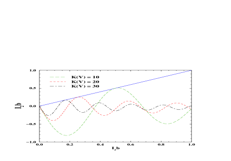
Figure 1: A graphical solution of Eq. (12) for $T=10$ MeV and $\tau=1.825$. The l.h.s. (straight line) and r.h.s. of Eq. (12) (all dashed curves) are shown as the function of dimensionless parameter $I_{1}\,b$ for the three values of the largest fragment size $K(V)$. The intersection point at $(0;\,0)$ corresponds to a real root of Eq. (10). Each tangent point with the straight line generates two complex roots of (10).

IV No Phase Transition Case

It is instructive to treat the effective chemical potential $\nu(\lambda)$ as an independent variable instead of $\mu$. In contrast to the infinite $V$, where the upper limit $\nu\leq 0$ defines the liquid phase singularity of the isobaric partition and gives the pressure of a liquid phase $p_{l}(T,\mu)=TR_{0}|_{V\rightarrow\infty}=(\mu+W(T))/b$ Bugaev:00 ; Bugaev:01 , for finite volumes and finite $K(V)$ the effective chemical potential can be complex (with either sign for its real part) and its value defines the number and position of the imaginary roots $\{\lambda_{n>0}\}$ in the complex plane. Positive and negative values of the effective chemical potential for finite systems were considered Elliott:01 within the Fisher droplet model, but, to our knowledge, its complex values have never been discussed. From the definition of the effective chemical potential $\nu(\lambda)$ it is evident that its complex values for finite systems exist only because of the excluded volume interaction, which is not taken into account in the Fisher droplet model Fisher:67 .

As it is seen from Fig. 1, the r.h.s. of Eq. (12) is the amplitude and frequency modulated sine-like function of dimensionless parameter $I_{n}\,b$. Therefore, depending on $T$ and $Re(\nu)$ values, there may exist no complex roots $\{\lambda_{n>0}\}$, a finite number of them, or an infinite number of them. In Fig. 1 we showed a special case which corresponds to exactly three roots of Eq. (10) for each value of $K(V)$: the real root ($I_{0}=0$) and two complex conjugate roots ($\pm I_{1}$). Since the r.h.s. of (12) is monotonously increasing function of $Re(\nu)$, when the former is positive, it is possible to map the $T-Re(\nu)$ plane into regions of a fixed number of roots of Eq. (10). Each curve in Fig. 2 divides the $T-Re(\nu)$ plane into three parts: for $Re(\nu)$-values below the curve there is only one real root (gaseous phase), for points on the curve there exist three roots, and above the curve there are five or more roots of Eq. (10).

For constant values of $K(V)\equiv K$ the number of terms in the r.h.s. of (12) does not depend on the volume and, consequently, in thermodynamic limit $V\rightarrow\infty$ only the farthest right simple pole in the complex $\lambda$-plane survives out of a finite number of simple poles. According to the inequality (13), the real root $\lambda_{0}$ is the farthest right singularity of isobaric partition (6). However, there is a possibility that the real parts of other roots $\lambda_{n>0}$ become infinitesimally close to $R_{0}$, when there is an infinite number of terms which contribute to the GCP (9).

Figure 2: Each curve separates the $T-Re(\nu_{n})$ region of one real root of Eq. (10) (below the curve), three complex roots (at the curve) and five and more roots (above the curve) for three values of $K(V)$ and the same parameters as in Fig. 1.

Let us show now that even for an infinite number of simple poles in (9) only the real root $\lambda_{0}$ survives in the limit $V\rightarrow\infty$. For this purpose consider the limit $Re(\nu_{n})\gg T$. In this limit the distance between the imaginary parts of the nearest roots remains finite even for infinite volume. Indeed, for $Re(\nu_{n})\gg T$ the leading contribution to the r.h.s. of (12) corresponds to the harmonic with $k=K$, and, consequently, an exponentially large amplitude of this term can be only compensated by a vanishing value of $\sin\left(I_{n}\,bK\right)$, i.e. $I_{n}\,bK=\pi n+\delta_{n}$ with $|\delta_{n}|\ll\pi$ (hereafter we will analyze only the branch $I_{n}>0$), and, therefore, the corresponding decay/formation time $\tau_{n}\approx K[\pi nT]^{-1}$ is volume independent.

Keeping the leading term on the r.h.s. of (12) and solving for $\delta_{n}$, one finds

$$I_{n} \approx (-1)^{n+1}\tilde{\phi}_{K}(T)~{}{\textstyle e^{\frac{Re(\nu_{n})\,K}{T}}}~{}\delta_{n}\,,$$ (14)

$$\delta_{n} \approx \frac{(-1)^{n+1}\pi n}{Kb~{}\tilde{\phi}_{K}(T)}~{}{\textstyle e^{-\frac{Re(\nu_{n})\,K}{T}}}\,,$$ (15)

$$R_{n} \approx (-1)^{n}\tilde{\phi}_{K}(T)~{}{\textstyle e^{\frac{Re(\nu_{n})\,K}{T}}}\,,$$ (16)

where in the last step we used Eq. (11) and condition $|\delta_{n}|\ll\pi$. Since for $V\rightarrow\infty$ all negative values of $R_{n}$ cannot contribute to the GCP (9), it is sufficient to analyze even values of $n$ which, according to (16), generate $R_{n}>0$.

Since the inequality (13) can not be broken, a single possibility, when $\lambda_{n>0}$ pole can contribute to the partition (9), corresponds to the case $R_{n}\rightarrow R_{0}-0^{+}$ for some finite $n$. Assuming this, we find $Re(\nu(\lambda_{n}))\rightarrow Re(\nu(\lambda_{0}))$ for the same value of $\mu$.

Substituting these results into equation (11), one gets

$$R_{n}\approx\sum\limits_{k=1}^{K}\tilde{\phi}_{k}(T)~{}{\textstyle e^{\frac{Re(\nu(\lambda_{0}))\,k}{T}}}\cos\left[\frac{\pi nk}{K}\right]\ll R_{0}\,.$$ (17)

The inequality (17) follows from the equation for $R_{0}$ and the fact that, even for equal leading terms in the sums above (with $k=K$ and even $n$), the difference between $R_{0}$ and $R_{n}$ is large due to the next to leading term $k=K-1$, which is proportional to $e^{\frac{Re(\nu(\lambda_{0}))\,(K-1)}{T}}\gg 1$. Thus, we arrive at a contradiction with our assumption $R_{0}-R_{n}\rightarrow 0^{+}$, and, consequently, it cannot be true. Therefore, for large volumes the real root $\lambda_{0}$ always gives the main contribution to the GCP (9), and this is the only root that survives in the limit $V\rightarrow\infty$. Thus, we showed that the model with the fixed size of the largest fragment has no phase transition because there is a single singularity of the isobaric partition (6), which exists in thermodynamic limit.

V Finite Volume Analogs of Phases

If $K(V)$ monotonically grows with the volume, the situation is different. In this case for positive value of $Re(\nu)\gg T$ the leading exponent in the r.h.s. of (12) also corresponds to a largest fragment, i.e. to $k=K(V)$. Therefore, we can apply the same arguments which were used above for the case $K(V)=K=const$ and derive similarly equations (14)–(16) for $I_{n}$ and $R_{n}$. From $I_{n}\approx\frac{\pi n}{b\,K(V)}$ it follows that, when $V$ increases, the number of simple poles in (III) also increases and the imaginary part of the closest to the real $\lambda$-axis poles becomes very small, i.e $I_{n}\rightarrow 0$ for $n\ll K(V)$, and, consequently, the associated decay/formation time $\tau_{n}\approx K(V)[\pi nT]^{-1}$ grows with the volume of the system. Due to $I_{n}\rightarrow 0$, the inequality (17) cannot be established for the poles with $n\ll K(V)$. Therefore, in contrast to the previous case, for large $K(V)$ the simple poles with $n\ll K(V)$ will be infinitesimally close to the real axis of the complex $\lambda$-plane.

From Eq. (16) it follows that

$$R_{n}~{}\approx~{}\frac{p_{l}(T,\mu)}{T}-\frac{1}{K(V)b}\ln\left|\frac{R_{n}}{\tilde{\phi}_{K}(T)}\right|\rightarrow\frac{p_{l}(T,\mu)}{T}$$ (18)

for $|\mu|\gg T$ and $K(V)\rightarrow\infty$. Thus, we proved that for infinite volume the infinite number of simple poles moves toward the real $\lambda$-axis to the vicinity of liquid phase singularity $\lambda_{l}=p_{l}(T,\mu)/T$ of the isobaric partition Bugaev:00 ; Bugaev:01 and generates an essential singularity of function ${\cal F}(V,p_{l}/T)$ in (II) irrespective to the sign of chemical potential $\mu$. As we showed above, the states with $Re(\nu)\gg T$ become stable because they acquire infinitely large decay/formation time $\tau_{n}$ in the limit $V\rightarrow\infty$. Therefore, these states should be identified as a liquid phase for finite volumes as well. Such a conclusion can be easily understood, if we recall that the partial pressure $TR_{n}$ of (18) corresponds to a single fragment of the largest possible size.

Now it is clear that each curve in Fig. 2 is the finite volume analog of the phase boundary $T-\mu$ for a given value of $K(V)$: below the phase boundary there exists a gaseous phase, but at and above each curve there are states which can be identified with a finite volume analog of the mixed phase, and, finally, at $Re(\nu)\gg T$ there exists a liquid phase. When there is no phase transition, i.e. $K(V)=K=const$, the structure of simple poles is similar, but, first, the line which separates the gaseous states from the metastable states does not change with the volume, and, second, as shown above, the metastable states will never become stable. Therefore, a systematic study of the volume dependence of free energy (or pressure for very large $V$) along with the formation and decay times may be of a crucial importance for experimental studies of the nuclear liquid gas phase transition.

The above results demonstrate that, in contrast to Hill’s expectations Hill , the finite volume analog of the mixed phase does not consist just of two pure phases. The mixed phase for finite volumes consists of a stable gaseous phase and the set of metastable states which differ by the free energy. Moreover, the difference between the free energies of these states is not surface-like, as Hill assumed in his treatment Hill , but volume-like. Furthermore, according to Eqs. (11) and (12), each of these states consists of the same fragments, but with different weights. As seen above for the case $Re(\nu)\gg T$, some fragments that belong to the states, in which the largest fragment is dominant, may, in principle, have negative weights (effective number of degrees of freedom) in the expression for $R_{n>0}$ (11). This can be understood easily because higher concentrations of large fragments can be achieved at the expense of the smaller fragments and is reflected in the corresponding change of the real part of the free energy $-R_{n>0}VT$. Therefore, the actual structure of the mixed phase at finite volumes is more complicated than was expected in earlier works.

A similar situation occurs for the real values of $K(V)$. In this case all sums in Eqs. (10-13) should be expressed via the Euler-MacLaurin formula

$$\sum\limits_{k=1}^{K(V)}f_{k}=f(1)+\int\limits_{2}^{K(V)}dk\,f(k)+{\textstyle\frac{f(K(V))+f(2)}{2}+\Delta_{f}(K)-}\,$$

$$\Delta_{f}(2)\,,{\rm where}\quad\Delta_{f}(z)=\sum\limits_{n=1}\frac{B_{2n}}{(2n)!}~{}\frac{d^{2n}f(x)}{d\,x^{2n}}\biggr{|}_{x=z}\,.$$ (19)

Here $B_{2n}$ are the Bernoulli numbers. The representation (19) allows one to study the effect of finite volume (FV) on the GCP (9).

The above results are valid for any $K(V)$ dependence. However, the linear one, i.e. $K(V)=\alpha V/b$ with $0<\alpha\leq 1$, is the most natural. With the help of the parameter $\alpha\leq 1$ it is possible to describe a difference between the geometrical shape of the volume under consideration and that one of the largest fragment. For instance, by fixing $\alpha=\pi/6$ it is possible to account for the fact that the largest spherical fragment cannot fill completely the cube with the side equal to its two radii, while there is enough space available for small fragments. Due to the $K(V)$ dependence in the CSMM there are two different ways of how the finite volume affects thermodynamical functions: for finite $V$ and $Re(\nu_{n})$ there is always a finite number of simple poles in (9), but their number and positions in the complex $\lambda$-plane depend on $V$. To see this, let us study the mechanical pressure which corresponds to the GCP (9)

$$p=T\frac{\partial\ln{\cal Z}(V,T,\mu)}{\partial V}={\textstyle\frac{T}{{\cal Z}(V,T,\mu)}}\sum\limits_{\{\lambda_{n}\}}\Biggl{[}\frac{\lambda_{n}~{}e^{\lambda_{n}\,V}}{1-\frac{\partial{\cal F}(V,\lambda_{n})}{\partial\lambda_{n}}}+$$

$$\frac{e^{\lambda_{n}\,V}}{\left[1-\frac{\partial{\cal F}(V,\lambda_{n})}{\partial\lambda_{n}}\right]^{2}}\Biggl{\{}b^{2}\,\frac{\partial\lambda_{n}}{\partial V}\sum\limits_{k=1}^{K(V)}\tilde{\phi}_{k}\,k^{2}~{}{\textstyle e^{\frac{\nu_{n}\,k}{T}}}+\tilde{\phi}_{K(V)}\times$$

$${\textstyle e^{\frac{\nu_{n}\,K(V)}{T}}}{\textstyle K(V)\left[1-\alpha+\frac{\nu_{n}}{T}\left(\frac{1}{2}-\alpha\right)\right]}+o(K(V))\Biggr{\}}\Biggr{]},$$ (20)

where we give the main term for each $\lambda_{n}$ and leading FV corrections explicitly for $Re(\nu_{n})/T<1$, whereas $o(K(V))$ accumulates the higher order corrections due to the Euler-MacLaurin Eq. (19). In evaluation of (V) we used an explicit representation of the derivative $\partial\lambda_{n}/\partial V$ which can be found from Eqs. (10) and (19). The first term in the r.h.s. of (V) describes the constrained grand canonical (CGC) complex pressure generated by the simple pole $\lambda_{n}$ (due to its free energy density $-\lambda_{n}T$) weighted with the “probability” $e^{\lambda_{n}\,V}/{\cal Z}(V,T,\mu)$, whereas the second and third terms appear due to the volume dependence of $K(V)$. Note that, instead of the FV corrections, the usage of natural values for $K(V)$ would generate the artificial delta-function terms in (V) for the volume derivatives. Now it is clear that in case $K(V)=K=const$ the corrections to the main term will not appear, and the number of poles and their positions will be defined by values of $T$ and $\mu$ only.

As one can see from (V), for finite volumes the corrections can give a non-negligible contribution to the pressure because in this case $Re(\nu_{n})>0$ can be positive. The real parts of the partial CGC pressures $T\lambda_{n}$ may have either sign. Therefore, if the FV corrections to the pressure (V) are small, then, according to (13), the positive CGC pressures $TR_{n>0}>0$ are mechanically metastable and the negative ones $TR_{n>0}<0$ are mechanically unstable compared to the gas pressure $TR_{0}$. The FV corrections should be accounted for to find the mechanically meta- and unstable states in the general case. However, it is clear that the contribution of the states with $TR_{n>0}<0$ into partition and its derivatives is exponentially small even for finite volumes.

As we showed earlier in this section, when $V$ increases, the number of simple poles in (III) also increases and imaginary part of the closest to the real $\lambda$-axis poles becomes very small. Therefore, for infinite volume the infinite number of simple poles moves toward the real $\lambda$-axis to the vicinity of liquid phase singularity $p_{l}(T,\mu)/T$ and, thus, generates an essential singularity of function ${\cal F}(V,p_{l}/T)$ in (II). In this case the contribution of any of remote poles from the real $\lambda$-axis to the GCP vanishes. Then it can be shown that the FV corrections in (V) become negligible because of the inequality $Re(\nu_{n})\leq 0$, and, consequently, the reduced distribution of largest fragment $\tilde{\phi}_{K(V)}(T)=K(V)^{-\tau}\,\exp(-\sigma(T)~{}K(V)^{2/3}/T)$ and the derivatives $\partial\lambda_{n}/\partial V$ vanish for all $T$-values, and we obtain the usual SMM solution Bugaev:00 ; Bugaev:01 . Its thermodynamics, as we discussed, is governed by the farthest right singularity in the complex $\lambda$-plane.

VI Conclusions

In this work we discussed a powerful mathematical method which allowed us to solve analytically the CSMM at finite volumes. It is shown that for finite volumes the GCP function can be identically rewritten in terms of the simple poles of the isobaric partition (6). The real pole $\lambda_{0}$ exists always and the quantity $T\lambda_{0}$ is the CGC pressure of the gaseous phase. The complex roots $\lambda_{n>0}$ appear as pairs of complex conjugate solutions of equation (10). As we discussed, their most straightforward interpretation is as follows: $-TRe(\lambda_{n>0})$ has a meaning of the free energy density, whereas $bTIm(\lambda_{n>0})$, depending on sign, gives the inverse decay/formation time of such a state. The gaseous state is always stable because its decay/formation time is infinite and because it has the smallest value of free energy. The complex poles describe the metastable states for $Re(\lambda_{n>0})\geq 0$ and mechanically unstable states for $Re(\lambda_{n>0})<0$.

We studied the volume dependence of the simple poles and found a dramatic difference in their behavior in case of phase transition and without it. For the former this representation allows one also to define the finite volume analogs of phases unambiguously and to establish the finite volume analog of the $T-\mu$ phase diagram (see Fig. 2). At finite volumes the gaseous phase exists, if there is a single simple pole, the mixed phase corresponds to three and more simple poles, whereas the liquid is represented by an infinite amount of simple poles at highest possible particle density (or $\mu\rightarrow\infty$).

As we showed, for given $T$ and $\mu$ the states of the mixed phase which have different $Re(\lambda_{n})$ are not in a true chemical equilibrium for finite volumes. This feature cannot be obtained within the Fisher droplet model due to lack of the hard core repulsion between fragments. This fact also demonstrates clearly that, in contrast to Hill’s expectations Hill , the mixed phase is not just a composition of two states which are the pure phases. As we showed, the mixed phase is a superposition of three and more collective states, and each of them is characterized by its own value of $\lambda_{n}$. Because of that the difference between the free energies of these states is not a surface-like, as Hill argued Hill , but volume-like.

For the case with phase transition, i.e. for $\frac{dK(V)}{d~{}V}>0$, we analyzed what happens in thermodynamic limit. When $V$ grows, the number of simple poles in (III) also increases and imaginary part of the closest to the real $\lambda$-axis poles becomes vanishing. For infinite volume the infinite number of simple poles moves toward the real $\lambda$-axis and forms an essential singularity of function ${\cal F}(V,p_{l}/T)$ in (II), which defines the liquid phase singularity $p_{l}(T,\mu)/T$. Thus, we showed how the phase transition develops in thermodynamic limit.

Also we analyzed the finite volume corrections to the mechanical pressure (V). The corrections of a similar kind should appear in the entropy, particle number and energy density because of the $T$ and $\mu$ dependence of $\lambda_{n}$ due to (10) Bugaev:04a . Therefore, these corrections should be taking into account while analyzing the experimental yields of fragments. Then the phase diagram of the nuclear liquid-gas phase transition can be recovered from the experiments on finite systems (nuclei) with more confidence.

A detailed analysis of the isobaric partition singularities in the $T-Re(\nu)$ plane allowed us to define the finite volume analogs of phases and study the behavior of these singularities in the limit $V\rightarrow\infty$. Such an analysis opens a possibility to study rigorously the nuclear liquid-gas phase transition directly from the finite volume partition. This may help to extract the phase diagram of the nuclear liquid-gas phase transition from the experiments on finite systems (nuclei) with more confidence.

Acknowledgments. This work was supported by the US Department of Energy. The fruitful discussions with J. B. Elliott and M. I. Gorenstein are appreciated.

References

- (1) J. P. Bondorf et al., Phys. Rep. 257 (1995) 131.
- (2) D. H. E. Gross, Phys. Rep. 279 (1997) 119.
- (3) L. G. Moretto et. al., Phys. Rep. 287 (1997) 249.
- (4) S. Das Gupta and A.Z. Mekjian, Phys. Rev. C 57 (1998) 1361.
- (5) S. Das Gupta, A. Majumder, S. Pratt and A. Mekjian, arXiv:nucl-th/9903007 (1999).
- (6) K. A. Bugaev, M. I. Gorenstein, I. N. Mishustin and W. Greiner, Phys. Rev. C62 (2000) 044320; arXiv:nucl-th/0007062 (2000).
- (7) K. A. Bugaev, M. I. Gorenstein, I. N. Mishustin and W. Greiner, Phys. Lett. B 498 (2001) 144; arXiv:nucl-th/0103075 (2001).
- (8) P. T. Reuter and K. A. Bugaev, Phys. Lett. B 517 (2001) 233.
- (9) K. A. Bugaev, arXiv:nucl-th/0406033 (2004).
- (10) K. A. Bugaev, L. Phair and J. B. Elliott, arXiv:nucl-th/0406034 (2004); K. A. Bugaev and J. B. Elliott, arXiv:nucl-th/0501080 (2005).
- (11) T. L. Hill, Thermodynamics of Small Systems (1994) Dover Publications, N. Y.
- (12) C. B. Das, S. Das Gupta and A. Z. Mekjian, Phys. Rev. C 68 (2003) 031601.
- (13) M. E. Fisher, Physics 3 (1967) 255.
- (14) M. I. Gorenstein, V. K. Petrov and G. M. Zinovjev, Phys. Lett. B 106 (1981) 327.
- (15) R. P. Feynman, “Statistical Mechanics”, Westview Press, Oxford, 1998.
- (16) J. B. Elliott et al. [ISiS Collaboration], Phys. Rev. Lett. 88 (2002) 042701.