Abstract

A $\gamma$-rigid solution of the Bohr Hamiltonian for $\gamma=30^{\rm o}$ is derived, its ground state band being related to the second order Casimir operator of the Euclidean algebra E(4). Parameter-free (up to overall scale factors) predictions for spectra and B(E2) transition rates are in close agreement to the E(5) critical point symmetry, as well as to experimental data in the Xe region around $A=130$.

1. Introduction

The E(5) [1] and X(5) [2] critical point symmetries, describing shape phase transitions from vibrational [U(5)] to $\gamma$-unstable [SO(6)] and vibrational to prolate deformed [SU(3)] nuclei respectively, have attracted recently much attention, since supporting experimental evidence is increasing [3, 4, 5, 6]. The E(5) model is obtained as an exact solution of the Bohr Hamiltonian [7] for $\gamma$-independent potentials [1], while the X(5) model is obtained as an approximate solution for $\gamma\approx 0^{\rm o}$ [2]. Another approximate solution, with $\gamma\approx 30^{\rm o}$, called Z(5), has also been obtained [8]. In all these cases, five degrees of freedom (the collective variables $\beta$, $\gamma$, and the three Euler angles) are taken into account.

In the present work we derive an exact solution of the Bohr Hamiltonian for $\gamma=30^{\rm o}$, by “freezing” $\gamma$ (as in Ref. [9]) to this value and taking into account only four degrees of freedom ($\beta$ and the Euler angles). In accordance to previous terminology, this solution will be called Z(4). It turns out that the Z(4) spectra and B(E2) transition rates are quite similar to the E(5) ones, while in parallel the ground state band of Z(4) is related to the Euclidean algebra E(4), thus offering the first clue of connection between critical point symmetries and Lie algebraic symmetries, in addition to the case of the E(5) model [1]. Experimental examples of Z(4) seem to appear in the Xe region around $A=130$.

The Z(4) solution will be introduced in Section 2 and its ground state band will be related to E(4) in Section 3. Numerical results and comparisons to E(5) and experiment will be given in Section 4, while discussion of the present results and plans for further work will appear in Section 5.

2. The Z(4) model

In the model of Davydov and Chaban [9] it is assumed that the nucleus is rigid with respect to $\gamma$-vibrations. Then the Hamiltonian depends on four variables ($\beta,\theta_{i}$) and has the form [9]

$$H=-\frac{\hbar^{2}}{2B}\Biggl{[}\frac{1}{\beta^{3}}\frac{\partial}{\partial\beta}\beta^{3}\frac{\partial}{\partial\beta}-\frac{1}{4\beta^{2}}\sum_{k=1}^{3}\frac{Q_{k}^{2}}{\sin^{2}(\gamma-\frac{2\pi}{3}k)}\Biggr{]}+U(\beta),$$ (1)

where $\beta$ and $\gamma$ are the usual collective coordinates [7], while $Q_{k}$ ($k=1$, 2, 3) are the components of angular momentum and $B$ is the mass parameter. In this Hamiltonian $\gamma$ is treated as a parameter and not as a variable. The kinetic energy term of Eq. (1) is different from the one appearing in the E(5) and X(5) models, because of the different number of degrees of freedom treated in each case (four in the former case, five in the latter).

Introducing [1] reduced energies $\epsilon=(2B/\hbar^{2})E$ and reduced potentials $u=(2B/\hbar^{2})U$, and considering a wave function of the form $\Psi(\beta,\theta_{i})=\phi(\beta)\psi(\theta_{i})$, where $\theta_{i}$ ( $i=1$, 2, 3) are the Euler angles, separation of variables leads to two equations

$$\Biggl{[}\frac{1}{\beta^{3}}\frac{\partial}{\partial\beta}\beta^{3}\frac{\partial}{\partial\beta}-\frac{\lambda}{\beta^{2}}+(\epsilon-u(\beta))\Biggr{]}\phi(\beta)=0,$$ (2)

$$\Biggl{[}\frac{1}{4}\sum_{k=1}^{3}\frac{Q_{k}^{2}}{\sin^{2}(\gamma-\frac{2\pi}{3}k)}-\lambda\Biggr{]}\psi(\theta_{i})=0.$$ (3)

In the case of $\gamma=\pi/6$, the last equation takes the form

$$\Biggl{[}\frac{1}{4}(Q_{1}^{2}+4Q_{2}^{2}+4Q_{3}^{2})-\lambda\Biggr{]}\psi(\theta_{i})=0.$$ (4)

This equation has been solved by Meyer-ter-Vehn [10], the eigenfunctions being

$$\psi(\theta_{i})=\psi^{L}_{\mu,\alpha}(\theta_{i})=\sqrt{\frac{2L+1}{16\pi^{2}(1+\delta_{\alpha,0})}}\,\Bigl{[}{\cal D}^{(L)}_{\mu,\alpha}(\theta_{i})+(-1)^{L}{\cal D}^{(L)}_{\mu,-\alpha}(\theta_{i})\Bigr{]}$$ (5)

with

$$\lambda=\lambda_{L,\alpha}=L(L+1)-\frac{3}{4}\,\alpha^{2},$$ (6)

where ${\cal D}(\theta_{i})$ denote Wigner functions of the Euler angles, $L$ are the eigenvalues of angular momentum, while $\mu$ and $\alpha$ are the eigenvalues of the projections of angular momentum on the laboratory fixed $\hat{z}$-axis and the body-fixed $\hat{x}^{\prime}$-axis respectively. $\alpha$ has to be an even integer [10].

Instead of the projection $\alpha$ of the angular momentum on the $\hat{x}^{\prime}$-axis, it is customary to introduce the wobbling quantum number [10, 11] $n_{w}=L-\alpha$, which labels a series of bands with $L=n_{w},n_{w}+2,n_{w}+4,\dots$ (with $n_{w}>0$) next to the ground state band (with $n_{w}=0$) [10].

The “radial” Eq. (2) is exactly soluble in the case of an infinite square well potential ($u(\beta)=0$ for $\beta\leq\beta_{W}$, $u(\beta)=\infty$ for $\beta>\beta_{W}$). Using the transformation $\phi(\beta)=\beta^{-1}f(\beta)$, Eq. (2) becomes a Bessel equation

$$\Biggl{[}\frac{\partial^{2}}{\partial\beta^{2}}+\frac{1}{\beta}\frac{\partial}{\partial\beta}+\Bigl{(}\epsilon-\frac{\nu^{2}}{\beta^{2}}\Bigr{)}\Biggr{]}f(\beta)=0,$$ (7)

with

$$\nu=\sqrt{\lambda+1}=\sqrt{L(L+1)-\frac{3}{4}\,\alpha^{2}+1}={\sqrt{L(L+4)+3n_{w}(2L-n_{w})+4}\over 2}.$$ (8)

Then the boundary condition $f(\beta_{W})=0$ determines the spectrum,

$$\epsilon_{\beta;s,\nu}=\epsilon_{\beta;s,n_{w},L}=(k_{s,\nu})^{2},\qquad k_{s,\nu}={x_{s,\nu}\over\beta_{W}},$$ (9)

where $x_{s,\nu}$ is the $s$th zero of the Bessel function $J_{\nu}(z)$. The eigenfunctions are

$$\phi(\beta)=\phi_{s,\nu}(\beta)=\phi_{s,n_{w},L}(\beta)=\frac{1}{\sqrt{c}}\,\beta^{-1}J_{\nu}(k_{s,\nu}\beta),\qquad\qquad c=\frac{\beta_{W}^{2}}{2}\,J^{2}_{\nu+1}(x_{s,\nu})$$ (10)

where the normalization constant $c$ is determined from the condition $\int_{0}^{\beta_{W}}\beta^{3}\phi^{2}(\beta)d\beta=1$. The notation for the roots has been kept the same as in Ref. [2], while for the energies the notation $E_{s,n_{w},L}$ will be used. The ground state band corresponds to $s=1$, $n_{w}=0$. This model will be called the Z(4) model.

The calculation of B(E2)s proceeds as in Ref. [8], the only difference being that the integrals over $\beta$ have the form

$$I_{\beta}(s_{i},L_{i},\alpha_{i};s_{f},L_{f},\alpha_{f})=\int_{0}^{\beta_{W}}\beta\,\phi_{s_{i},\nu_{i}}(\beta)\,\phi_{s_{f},\nu_{f}}(\beta)\,\beta^{3}d\beta,$$ (11)

since the volume element in the present case corresponds to four dimensions instead of five.

A brief discussion of the interrelations among various triaxial models is now in place. In the original triaxial model of Davydov and Filippov [12], the Hamiltonian contains only a rotational term [the second term in Eq. (1)], and is analytically soluble for all values of $\gamma$. In contrast, the Hamiltonian of Davydov and Chaban [9] contains both a kinetic energy term [the first term in Eq. (1)] and a rotational term, and is solved numerically. Meyer-ter-Vehn [10] has shown that triaxial Hamiltonians including both a kinetic energy term and a rotational term are analytically soluble in the special case of $\gamma=30^{\rm o}$. In the present Z(4) case an analytical solution of the Davydov and Chaban Hamiltonian is obtained for the special case of $\gamma=30^{\rm o}$, as implied by Meyer-ter-Vehn.

3. Relation of the ground state band of Z(4) to E(4)

The ground state band of the Z(4) model is related to the second order Casimir operator of E(4), the Euclidean group in four dimensions. In order to see this, one can consider in general the Euclidean algebra in $n$ dimensions, E(n), which is the semidirect sum [13] of the algebra T_n of translations in $n$ dimensions, generated by the momenta

$$P_{j}=-i{\partial\over\partial x_{j}},$$ (12)

and the SO(n) algebra of rotations in $n$ dimensions, generated by the angular momenta

$$L_{jk}=-i\left(x_{j}{\partial\over\partial x_{k}}-x_{k}{\partial\over\partial x_{j}}\right),$$ (13)

symbolically written as E(n) = T_n $\oplus_{s}$ SO(n) [14]. The generators of E(n) satisfy the commutation relations

$$[P_{i},P_{j}]=0,\qquad[P_{i},L_{jk}]=i(\delta_{ik}P_{j}-\delta_{ij}P_{k}),$$ (14)

$$[L_{ij},L_{kl}]=i(\delta_{ik}L_{jl}+\delta_{jl}L_{ik}-\delta_{il}L_{jk}-\delta_{jk}L_{il}).$$ (15)

From these commutation relations one can see that the square of the total momentum, $P^{2}$, is a second order Casimir operator of the algebra, while the eigenfunctions of this operator satisfy the equation

$$\left(-{1\over r^{n-1}}{\partial\over\partial r}r^{n-1}{\partial\over\partial r}+{\omega(\omega+n-2)\over r^{2}}\right)F(r)=k^{2}F(r),$$ (16)

in the left hand side of which the eigenvalues of the Casimir operator of SO(n), $\omega(\omega+n-2)$ appear [15]. Putting

$$F(r)=r^{(2-n)/2}f(r),$$ (17)

and

$$\nu=\omega+{n-2\over 2},$$ (18)

Eq. (16) is brought into the form

$$\left({\partial^{2}\over\partial r^{2}}+{1\over r}{\partial\over\partial r}+k^{2}-{\nu^{2}\over r^{2}}\right)f(r)=0,$$ (19)

the eigenfunctions of which are the Bessel functions $f(r)=J_{\nu}(kr)$ [16]. The similarity between Eqs. (19) and (7) is clear.

The ground state band of Z(4) is characterized by $n_{w}=0$, which means that $\alpha=L$. Then Eq. (8) leads to $\nu=L/2+1$, while Eq. (18) in the case of E(4) gives $\nu=\omega+1$. Then the two results coincide for $L=2\omega$, i.e. for even values of $L$. One can easily see that this coincidence occurs only in four dimensions.

4. Numerical results and comparisons to E(5) and experiment

The lowest bands of the Z(4) model are given in Table 1. The notation $L_{s,n_{w}}$ is used. All levels are measured from the ground state, $0_{1,0}$, and are normalized to the first excited state, $2_{1,0}$. The ground state band is characterized by $s=1$, $n_{w}=0$, while the even and the odd levels of the $\gamma_{1}$-band are characterized by $s=1$, $n_{w}=2$, and $s=1$, $n_{w}=1$ respectively, and the $\beta_{1}$-band is characterized by $s=2$, $n_{w}=0$. These bands are also shown in Fig. 1, labelled by $(s,n_{w})$.

Both intraband and interband B(E2) transition rates, normalized to the one between the two lowest states, B(E2;$2_{1,0}\to 0_{1,0}$), are given in Fig. 1 .

The similarity between the spectra and B(E2) values of Z(4) and E(5), for which extensive numerical results can be found in Ref. [17], can be seen in Figs. 2(a) and 2(b), where the spectra of the ground state band and the $\beta_{1}$ band, as well as their intraband B(E2)s are given. One can easily check that the similarity extends to interband transitions between these bands as well, for which the selection rules in the two models are the same.

The main difference between Z(4) and E(5) appears, as expected, in the $\gamma_{1}$ band, the spectrum of which is shown in Fig. 2(c). The predictions of the two models for the odd levels practically coincide, while the predictions for the even levels differ, since in the E(5) model the levels are exactly paired as (3,4), (5,6), (7,8), …, as imposed by the underlying SO(5)$\supset$SO(3) symmetry [1, 17], while in the Z(4) model the levels are approximately paired as (4,5), (6,7), (8,9), …, which is a hallmark of rigid triaxial models [12]. The latter behaviour is never materialized fully [18], but it is known [19] that $\gamma$-unstable models and $\gamma$-rigid models yield similar predictions for most observables if $\gamma_{rms}$ of the former equals $\gamma_{rigid}$ of the latter, a situation occuring in the Ru-Pd, Xe-Ba (below $N=82$), and Os-Pt regions.

Predictions of the Z(4) model are compared to existing experimental data for ¹²⁸Xe [20], ¹³⁰Xe [21], and ¹³²Xe [22] in Fig. 3. The reasonable agreement observed is in no contradiction with the characterization of these nuclei as O(6) nuclei [19], since, as mentioned above, the predictions of $\gamma$-unstable models (like O(6) [23]) and $\gamma$-rigid models (like Z(4)) for most observables are similar if $\gamma_{rms}$ of the former equals $\gamma_{rigid}$ of the latter.

5. Discussion

In the present work an exact solution of the Bohr Hamiltonian with $\gamma$ “frozen” to $30^{\rm o}$, called Z(4), is obtained. Spectra and B(E2) transition rates of Z(4) resemble these of the critical point symmetry E(5), while the ground state band of Z(4) is related to the Euclidean algebra E(4), thus offering a first clue of connection between critical point symmetries and Lie algebras, in addition to the case of the E(5) model [1]. Empirical evidence for Z(4) in the Xe region around $A=130$ has been presented.

It should be emphasized, however, that neither the similarity of spectra and B(E2) values of Z(4) to these of the E(5) model, nor the coincidence of the ground state band of Z(4) to the spectrum of the Casimir operator of the Euclidean algebra E(4) clarify the algebraic structure of the Z(4) model, the symmetry algebra of which has to be constructed explicitly, starting from the fact that $\gamma$ is fixed to $30^{\rm o}$. The fact that the Bohr Hamiltonian for $\gamma=30^{\rm o}$ possesses “accidentally” a symmetry axis (the body-fixed $\hat{x}^{\prime}$-axis) has been early realized [24]. This “accidental” symmetry should also serve as the starting point for clarifying the symmetry underlying other solutions of the Bohr Hamiltonian obtained for $\gamma=30^{\rm o}$ [8, 25, 26].

Acknowledgements

One of the authors (IY) is thankful to the Turkish Atomic Energy Authority (TAEK) for support under project number 04K120100-4.

Table 1: Energy levels of the Z(4) model, measured from the $L_{s,n_{w}}=0_{1,0}$ ground state and normalized to the $2_{1,0}$ lowest excited state.

$s,n_{w}$	1,0	1,2	2,0		1,1
$L$				$L$
0	0.000		2.954
2	1.000	1.766	4.804	3	2.445
4	2.226	4.051	6.893	5	4.239
6	3.669	6.357	9.215	7	6.188
8	5.324	8.788	11.765	9	8.316
10	7.188	11.378	14.538	11	10.630
12	9.256	14.139	17.531	13	13.135
14	11.526	17.079	20.742	15	15.831
16	13.996	20.202	24.167	17	18.719
18	16.665	23.509	27.805	19	21.799
20	19.530	27.003	31.653	21	25.071

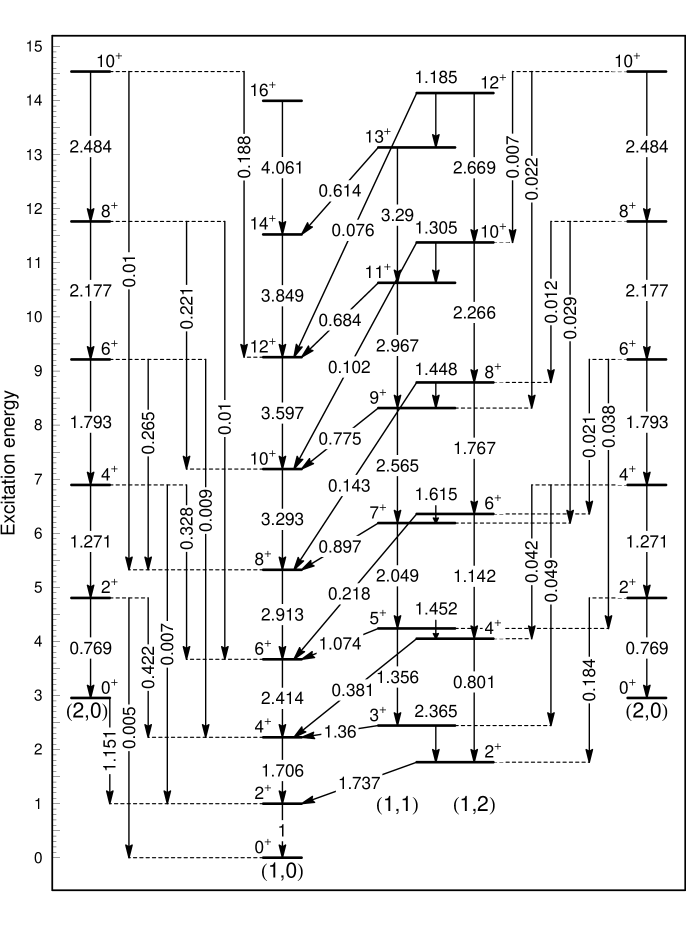
Figure 1: Intraband and interband B(E2) transition rates in the Z(4) model, normalized to the B(E2;$2_{1,0}\to 0_{1,0}$) rate. Bands are labelled by $(s,n_{w})$, their levels being normalized to $2_{1,0}$. The (2,0) band is shown both at the left and at the right end of the figure for drawing purposes.

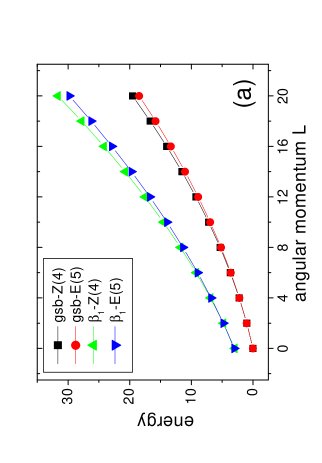
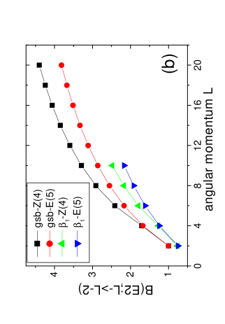
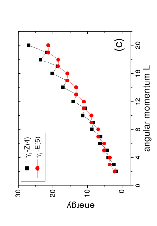
Figure 2: (a) Ground state band [$(s,n_{w})=(1,0)$] and first excited band [$(s,n_{w})=(2,0)$] of Z(4) (labeled as $\beta_{1}$-band) compared to the corresponding bands of E(5) [1, 17]. In each model all levels are normalized to the $2_{1}^{+}$ state. (b) Intraband B(E2) transition rates within the same bands of Z(4) compared to the corresponding B(E2) rates of E(5). In each model all rates are normalized to the $2_{1}^{+}\to 0_{1}^{+}$ rate. (c) The lowest“$K=2$ band” of Z(4) [formed out of the ($s,n_{w}$) bands (1,2) and (1,1), labeled as $\gamma_{1}$], compared to the corresponding band of E(5).

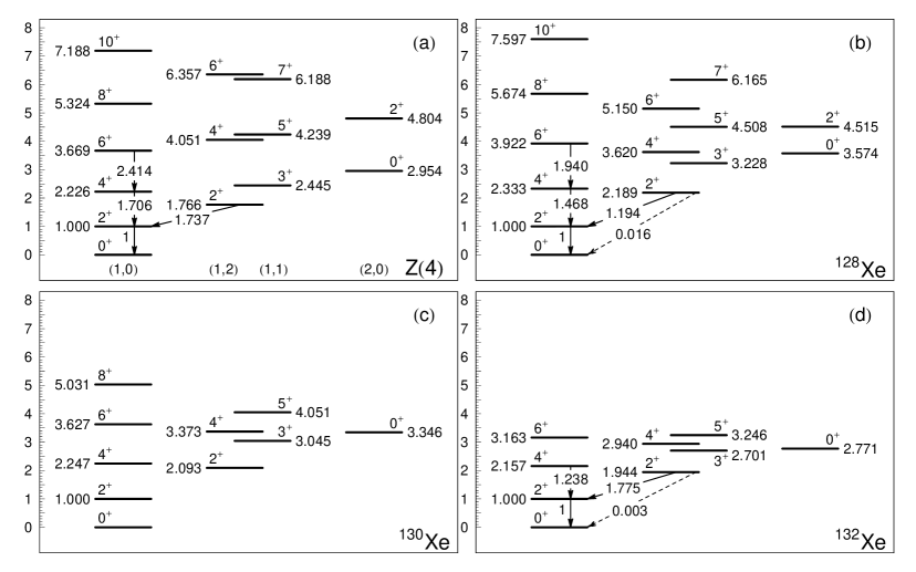
Figure 3: Comparison of the Z(4) predictions for (normalized) energy levels and (normalized) B(E2) transition rates (a) to experimental data for ¹²⁸Xe [20] (b), ¹³⁰Xe [21] (c), and ¹³²Xe [22] (d). Bands in (a) are labelled by $(s,n_{w})$. See Section 4 for further discussion.

References

- [1] F. Iachello, Phys. Rev. Lett. 85 (2000) 3580.
- [2] F. Iachello, Phys. Rev. Lett. 87 (2001) 052502.
- [3] R. F. Casten and N. V. Zamfir, Phys. Rev. Lett. 85 (2000) 3584.
- [4] R. M. Clark et al., Phys. Rev. C 69 (2004) 064322.
- [5] R. F. Casten and N. V. Zamfir, Phys. Rev. Lett. 87 (2001) 052503.
- [6] R. M. Clark et al., Phys. Rev. C 68 (2003) 037301.
- [7] A. Bohr, Mat. Fys. Medd. K. Dan. Vidensk. Selsk. 26 (1952) no. 14.
- [8] D. Bonatsos, D. Lenis, D. Petrellis, and P. A. Terziev, Phys. Lett. B 588 (2004) 172.
- [9] A. S. Davydov and A. A. Chaban, Nucl. Phys. 20 (1960) 499.
- [10] J. Meyer-ter-Vehn, Nucl. Phys. A 249 (1975) 111.
- [11] A. Bohr and B. R. Mottelson, Nuclear Structure, vol. II, Benjamin, New York, 1975.
- [12] A. S. Davydov and G. F. Filippov, Nucl. Phys. 8 (1958) 237.
- [13] B. G. Wybourne, Classical Groups for Physicists, Wiley, New York, 1974.
- [14] A. O. Barut and R. Raczka, Theory of Group Representations and Applications, World Scientific, Singapore, 1986.
- [15] M. Moshinsky, J. Math. Phys. 25 (1984) 1555.
- [16] M. Abramowitz and I. A. Stegun, Handbook of Mathematical Functions, Dover, New York, 1965.
- [17] D. Bonatsos, D. Lenis, N. Minkov, P. P. Raychev, and P. A. Terziev, Phys. Rev. C 69 (2004) 044316.
- [18] N. V. Zamfir and R. F. Casten, Phys. Lett. B 260 (1991) 265.
- [19] R. F. Casten, Nuclear Structure from a Simple Perspective, Oxford University Press, Oxford, 1990.
- [20] M. Kanbe and K. Kitao, Nucl. Data Sheets 94 (2001) 227.
- [21] B. Singh, Nucl. Data Sheets 93 (2001) 33.
- [22] Yu. Khazov, A. A. Rodionov, S. Sakharov, and B. Singh, Nucl. Data Sheets 104 (2005) 497.
- [23] F. Iachello, A. Arima, The Interacting Boson Model, Cambridge Univ. Press, Cambridge, 1987.
- [24] D. M. Brink, Prog. Nucl. Phys. 8 (1960) 99.
- [25] R. V. Jolos, Yad. Fiz. 67 (2004) 955 [Phys. At. Nucl. 67 (2004) 931].
- [26] L. Fortunato, Phys. Rev. C 70 (2004) 011302(R).