Complementary reaction analyses and the isospin mixing of the 4^- states in ¹⁶O.

Abstract

Data from the inelastic scattering of electrons, and of intermediate energy protons and pions leading to “stretched” configuration 4^- states near 19 MeV excitation in ¹⁶O as well as from charge exchange $(p,n)$ scattering to an isobaric analogue (4^-) state in ¹⁶F have been analyzed to ascertain the degree of isospin mixing contained within those states and of the amount of $d_{5/2}-p_{3/2}^{-1}$ particle-hole excitation strength they exhaust. The electron and proton scattering data have been analyzed using microscopic models of the structure and reactions, with details constrained by analyses of elastic scattering data.

I Introduction

The nucleus is an unique environment in that the strong, electromagnetic, and weak interactions all contribute in ways that are manifest in its static and dynamic attributes. Furthermore, as nuclear systems display a rich array of properties, it is not surprising that diverse reaction studies, using a variety of probes and processes, are required to provide a range of complementary information before a detailed understanding of nuclear structure is possible. A requirement is that the reaction mechanisms of importance in each use (types and specifications) are well known.

With the electromagnetic interaction, for both $\gamma$-decay probabilities and electron scattering form factors that supposition is well founded Uberall (1971), at least for momentum transfers to $\sim$ 3 fm^-1. At higher momentum transfer values, meson exchange current (MEC) corrections may have noticeable effect particularly on transverse form factors. For electric transitions, other studies Friar and Fallieros (1984, 1985) have shown how effective operators can be defined to account for MEC effects. With large basis shell model calculations of structure those corrections have led to good agreement with $E2$ transition data Karataglidis et al. (1995a); Amos et al. (2000). Magnetic transverse form factors also are affected by MEC, but as their evaluations explicitly involve the nuclear currents, individual MEC diagrams must be evaluated. While the one pion exchange current (seagull and pion in flight) contributions have little effect at small linear momentum transfer values in scattering to states involving large angular momentum change, they have some effect at higher momentum transfer values and do so in the case of the $M4$ values in ¹⁶O Hyde-Wright et al. (1987), though the effects are still minor and lie within vagaries of the choice of single nucleon bound state wave functions Clausen et al. (1988).

Data from the inelastic pion scattering from nuclei are of particular interest, especially for pions with energies that ensure the $\Delta$ resonance dominance of the underlying pion-nucleon ($\pi N$) interactions effecting the transitions. The interest stems largely from the distinctive relative transition strengths of $\pi^{+}$ and $\pi^{-}$ interactions with protons and neutrons. As a consequence, $\pi^{(\pm)}$ inelastic scattering cross sections should be sensitive to the isospin of (and so isospin mixing in) the nuclear states. But the specifics of the $\pi N$ $g$-matrices in nuclear matter are not well known.

In contrast, credible nucleon-nucleon ($NN$) $g$-matrices in the nuclear medium have been formed for an energy of an incoming nucleon from 25 to 250 MeV. Using effective interactions that map to those $g$-matrices, microscopic model (nonlocal) nucleon-nucleus optical potentials have been determined with which very good predictions of cross sections and spin observables from the elastic scattering of nucleons with energies in that range and from nuclei that span the mass table Amos et al. (2000). Such model evaluations of proton elastic scattering from ^6,8He Lagoyannis et al. (2001), and from ²⁰⁸Pb Karataglidis et al. (2002); Dupuis et al. (2005), gave estimates for the neutron skin thickness of each nuclei. Specifically, calculations of nucleon elastic scattering were made using complex, spin-dependent, and nonlocal optical potentials formed by folding an effective two-nucleon ($NN)$ interaction with nuclear state density matrices from a large basis space shell model calculation. That effective $NN$ interaction accurately maps to the $NN$ $g$-matrices half off the energy shell, solutions of the Brueckner-Bethe-Goldstone (BBG) equations for nuclear matter found for diverse Fermi momenta to 1.6 fm^-1 and built upon the BonnB $NN$ potentials. The nonlocal optical potentials so formed were used also to specify the continuum waves in a Distorted Wave Approximation (DWA) study of inelastic scattering. The effective $NN$ interaction was also used as the transition operator in those DWA calculations as was a large basis space shell model spectroscopy for the nuclear states. Remarkably good comparisons with data resulted, requiring no arbitrary renormalization or adjustments to bound state wave functions Amos et al. (2000). The inelastic scattering results so found, cross correlated extremely well with the electron scattering form factor predictions of the selected model of nuclear structure.

The study of transitions to the 4^- states in ¹⁶O is particularly interesting. First, the dominant spectroscopy of the residual states should be particle-hole excitations ($d_{5/2}-p_{3/2}^{-1}$) upon the ¹⁶O ground state. If an essentially closed shell model for that ground state is considered, only two such states should exist; one each with isospin ($T$) of 0 and 1. But there are four known 4^- states in the adopted spectrum Pearlman (1993) in the vicinity of 19 MeV excitation; the three lowest having observable excitation strength from the ground with one or more of the scattering of electrons, pions and protons. Two of those are dominantly isoscalar. The third is classified as an isovector state whose analogue in ¹⁶F has been seen in charge exchange $(p,n)$ experiments Anderson et al. (1979); Madey et al. (1982); Ohnuma et al. (1982). Furthermore, electron scattering (transverse) form factors for two of those states have been measured and analyzed Hyde-Wright et al. (1987); Clausen et al. (1988), $\pi^{(\pm)}$ inelastic scattering cross sections for energies in the $\Delta$ resonance region have been studied Holtkamp et al. (1980), and the cross section from inelastic scattering and cross section and analyzing power from charge exchange scattering of 135 MeV protons have been reported Henderson et al. (1979); Madey et al. (1982).

In the next section, the spectroscopy of the $4^{-}$ states is discussed giving a particle-hole model for their excitation (from the ground) and also a prescription to study configuration and isospin mixing among them. Then in Sec. III a brief outline of details of the calculations of electron, pion, and proton inelastic scattering and of charge exchange scattering to the isobaric analogue state (IAS) state in ¹⁶F is presented. The results of those calculations are then shown in Sec. IV and conclusions we draw follow in Sec. V.

II The spectroscopy of the 4^- states

Simple shell model calculations of ¹⁶O readily predict two 4^- states in the spectrum. These are the isoscalar and isovector combinations of the “stretched” particle-hole excitations upon the ground state with a $p_{3/2}$ proton(neutron) moving to the $d_{5/2}$ orbit. The best of such simple model calculations  Millener and Kurath (1975) predict excitation energies for those states of 19 MeV in accord with observation. The transition strength for excitation of such “stretched” states however, depends upon the fractional occupancies of the $p_{3/2}$ and $d_{5/2}$ orbits in the ground state. So one must have a good description for the ground state as well. The fractional occupancies can have a marked effect upon the normalization of cross-section peak values as was noted in a study of the excitation of the isoscalar/isovector pair of 6^- states in ²⁸Si Smith et al. (1978) wherein it was shown that using a large basis projected Hartree-Fock specification of the ground state could halve the strength of transition obtained from using a packed shell model description.

Diminution of particle-hole excitation strength may be anticipated with any “stretched” states isospin pair. But in the case of ¹⁶O, there are three strongly excited 4^- states in the region of 19 MeV excitation. Specifically they have excitation energies of 17.775, 18.977 and 19.808 MeV and (dominant) isospin values of 0, 1, and 0 respectively Pearlman (1993). There is a fourth listed now Pearlman (1993) at an excitation of 20.5 MeV to which we do not have scattering data. Additional isoscalar negative parity states are not unexpected though as such are noted in the evaluated spectrum as well as being predicted by shell model calculations that allow $3p-3h$ excitations Millener and Kurath (1975). But various questions about the distribution of ($d_{5/2}-p_{3/2}^{-1}$) strengths among these states ensue, as does the question of how much isospin mixing occurs.

Particle transfer reactions, e.g. ¹⁷O($d,t$) and ¹⁷O($d,{}^{3}$He) to these 4^- states give some useful indication of the ($d_{5/2}-p_{3/2}^{-1}$) strength distributions Mairle et al. (1978). Assuming that the reactions occur by direct population of the $1p-1h$ components of the residual states, the spectroscopic factors ($C^{2}S$) in the pure isospin limit must satisfy sum rules, namely

$$\sum(C^{2}S)_{(d,t)}=C^{2}S_{(d,{}^{3}{\rm He})}\ ,$$ (1)

and

$$(C^{2}S)_{(d,t)}|_{(T=1)}=\frac{1}{2}C^{2}S_{(d,{}^{3}{\rm He})}\ .$$ (2)

These relationships are satisfied approximately by experiment, and the extracted values for each transition suggest that the isovector (18.977) state contains 97% of the isovector particle-hole strength while the summed result of excitation of the (isoscalar) 17.775 and 19.808 MeV states would account for 92% of that strength. But extracted spectroscopic factors are very model dependent. Such percentages should be considered indicative at best.

II.1 A particle-hole model of the 4^- excitations in ¹⁶O

Denoting the ground state of ¹⁶O by $\left|J^{\pi};T\right\rangle=\left|0^{+};0\right\rangle$, a simple model for the 4^-;$T_{f}$ states is

$$\left|4^{-};T_{f}\right\rangle=\left|(p_{\frac{3}{2}}^{-1}d_{\frac{5}{2}})\,4^{-};T_{f}\right\rangle={\cal N}\left[a^{\dagger}_{\left(\frac{5}{2},\frac{1}{2}\right)}\times{\tilde{a}}^{\phantom{\dagger}}_{\left(\frac{3}{2},\frac{1}{2}\right)}\right]^{(4,T_{f})}_{(M_{4},M_{T_{f}=0})}\left|0^{+};0\right\rangle\ ,$$ (3)

in which the particle-hole operator has been coupled in both angular momentum and isospin; the brackets surrounding the subscripts on the creation and annihilation operators indicate that full coupling. This operator is defined by

$$\left[a^{\dagger}_{\left(\frac{5}{2},\frac{1}{2}\right)}\times{\tilde{a}}^{\phantom{\dagger}}_{\left(\frac{3}{2},\frac{1}{2}\right)}\right]^{(4,T_{f})}_{(M_{4},0)} =\sum(-)^{\left(\frac{3}{2}-m_{3}\right)}\left\langle\frac{3}{2}\,\frac{5}{2}\,m_{3}\,-m_{5}\Bigl{|}4\,-M_{4}\right\rangle$$ (4)

$$(-)^{\left(\frac{1}{2}-\alpha\right)}\left\langle\frac{1}{2}\,\frac{1}{2}\,\alpha\,-\alpha\Bigl{|}T_{f}\,0\right\rangle\ a^{\dagger}_{\frac{5}{2}m_{5}\alpha}a^{\phantom{\dagger}}_{\frac{3}{2}m_{3}\alpha}\ .$$

The summation is taken over all component particle projection quantum numbers, and $M_{T}=0$ as we consider an $N=Z$ nucleus. Herein we do not consider any reverse amplitudes, i.e. $(p_{\frac{3}{2}}-d_{\frac{5}{2}}^{-1})$. They will have very much smaller probability amplitudes, and none if the $d_{5/2}$ orbit in the ground state is vacant. The normalization of both of these states then is fixed by the fractional occupancies $\sigma_{j}$ of nucleons of either type in the orbits ($j$) in the ground state. The normalization, as developed in Appendix A, is

$${\cal N}=\left[\left\{1-\sigma_{\frac{5}{2}}\right\}\sigma_{\frac{3}{2}}\right]^{-\frac{1}{2}}\ .$$ (5)

The same procedure allows a model of an IAS in ¹⁶F though an additional isospin projection changing operator need be included.

For inelastic scattering (or charge exchange leading to an IAS state in ¹⁶F) involving scattering from a nucleon in orbit $j_{1}$ with isospin $y$ and then leaving a nucleon in orbit $j_{2}$ with isospin $x$, the one body density matrix elements (OBDME),

$$S_{j_{1}j_{2}I}^{(x,y)}=\left<4^{-};T_{f}\left\|\left[a^{\dagger}_{j_{2}x}\otimes{\tilde{a}}^{\phantom{\dagger}}_{j_{1}y}\right]^{(I)}\ \right\|0^{+};0\right>\ ,$$ (6)

are required. Note that, in this case, only angular momentum is coupled in the specification of the operator. That is designated by the absence of brackets around the subscripts of the creation and annihilation operators and the use of $\otimes$ as coupling operator. Clearly the transfer quantum number is $I=4$ and the combinations of proton and neutron spectroscopic amplitudes must effect an isospin change equal to $T_{f}$.

For inelastic scattering to the 4^- states in ¹⁶O then, as developed in Appendix B.1,

$$S_{\frac{3}{2}\frac{5}{2}4}^{(x)}=\frac{3}{\sqrt{2}}\left\{\delta_{(T_{f}0)}+\delta_{(T_{f}1)}(-)^{\left(\frac{1}{2}-x\right)}\right\}\ \sqrt{\sigma_{\frac{3}{2}}\left[1-\sigma_{\frac{5}{2}}\right]}\ ,$$ (7)

while for the charge exchange ($p,n$) reaction to the IAS $4^{-}$ state in ¹⁶F, as the struck nucleon must be a neutron to effect the charge transfer, $y=\frac{1}{2}=-x$. Then, and as developed in Appendix B.2,

$$S_{\frac{3}{2}\frac{5}{2}4}^{(-\frac{1}{2},\frac{1}{2})}=\delta_{(T_{f}1)}\ 3\sqrt{\sigma_{\frac{3}{2}}\left[1-\sigma_{\frac{5}{2}}\right]}\ .$$ (8)

II.2 Configuration and isospin mixing

We presume that the ground state of ¹⁶O has good isospin ($T=0$), but configuration mixing will certainly reduce the $p_{3/2}$ occupancy from the closed shell value (of 4). A large basis shell model calculation (in a complete $(0+2)\hbar\omega$ space) has been made of the ¹⁶O ground state Karataglidis et al. (1995b) and that gave values for $(2j+1)\sigma_{j}$ respectively of 3.87 and 0.14 for the $0p_{3/2}$ and $0d_{5/2}$ shells. To describe the $4^{-}$ states however, we consider a simple three component basis space. The three states of that basis the a pure particle-hole isovector states and two isoscalar states,

$$\left|a\right> = \left|4^{-};T=1\right>\ =\left|(d_{\frac{5}{2}}p^{-1}_{\frac{3}{2}});\,4^{-};T=1\right>\ ,$$

$$\left|b\right> = \left|4^{-};T=0\right>\ =\left|(d_{\frac{5}{2}}p^{-1}_{\frac{3}{2}});\,4^{-};T=0\right>\ ,$$

$$\left|c\right> = \left|(np-nh)\;4^{-};T=0\right>\ .$$ (9)

With these it is possible to create states having both configuration and isospin mixing. In particular we suppose with this basis that there is an optimal prescription for the three states of interest in ¹⁶O namely,

$$\left(\begin{array}[]{c}\left|4^{-};E_{1}=17.775\right>\\ \left|4^{-};E_{2}=18.977\right>\\ \left|4^{-};E_{3}=19.808\right>\end{array}\right)=\left(\begin{array}[]{ccc}C_{1}(E_{1})&C_{0}(E_{1})&C_{np-nh}(E_{1})\\ C_{1}(E_{2})&C_{0}(E_{2})&C_{np-nh}(E_{2})\\ C_{1}(E_{3})&C_{0}(E_{3})&C_{np-nh}(E_{3})\end{array}\right)\;\left(\begin{array}[]{c}\left|a\right>\\ \left|b\right>\\ \left|c\right>\end{array}\right)\ .$$ (10)

We presume that the basis state $\left<c\right|$ cannot be excited by a simple particle-hole operator acting upon the ground state, so that the scattering amplitudes for the excitation of each state, $E_{i}$, then are weighted sums

$${\cal M}(E_{i})=C_{0}(E_{i}){\cal M}_{\left<b\right|}+C_{1}(E_{i}){\cal M}_{\left<a\right|}\ ,$$ (11)

where the matrix elements ${\cal M}_{\left<x\right|}$ are transition amplitudes for the excitation of the basis states $\left\langle a\right|\,(T=1)$ and $\left\langle b\right|\,(T=0)$. However, it is also convenient to express the ${\cal M}(E_{i})$ in a form

$${\cal M}(E_{1}) = N_{1}\ \left\{\cos(\epsilon_{1})\,{\cal M}_{T=0}+\sin(\epsilon_{1})\,{\cal M}_{T=1}\right\}$$

$${\cal M}(E_{2}) = N_{2}\ \left\{\cos(\epsilon_{2})\,{\cal M}_{T=1}+\sin(\epsilon_{2})\,{\cal M}_{T=0}\right\}$$

$${\cal M}(E_{3}) = N_{3}\ \left\{\cos(\epsilon_{3})\,{\cal M}_{T=0}+\sin(\epsilon_{3})\,{\cal M}_{T=1}\right\}\ ,$$ (12)

where $N=\sqrt{C_{0}^{2}+C_{1}^{2}}$ and $\cos(\epsilon)=C_{T}/N$. The coupling angle for each state $\epsilon_{i}$, and the scales $N_{i}$, are to be determined from data magnitudes of the measured cross sections. For evaluations however, individual proton and neutron amplitudes will be formed whence

$${\cal M}(E_{1}) = N_{1}\ \left\{\left[\cos(\epsilon_{1})+\sin(\epsilon_{1})\right]\,{\cal M}_{\pi}+\left[\cos(\epsilon_{1})-\sin(\epsilon_{1})\right]\,{\cal M}_{\nu}\right\}$$

$${\cal M}(E_{2}) = N_{2}\ \left\{\left[\sin(\epsilon_{2})-\cos(\epsilon_{2})\right]\,{\cal M}_{\pi}+\left[\sin(\epsilon_{2})+\cos(\epsilon_{2})\right]\,{\cal M}_{\nu}\right\}$$

$${\cal M}(E_{3}) = N_{3}\ \left\{\left[\cos(\epsilon_{3})+\sin(\epsilon_{3})\right]\,{\cal M}_{\pi}+\left[\cos(\epsilon_{3})-\sin(\epsilon_{3})\right]\,{\cal M}_{\nu}\right\}\ .$$ (13)

III Details of the scattering data analyses

A particle-hole structure model for three $4^{-}$ states in ¹⁶O has been used in the past Barker et al. (1981); Hyde-Wright et al. (1987); Clausen et al. (1988) to analyze transverse magnetic $M4$ form factors extracted from inelastic electron scattering measurements Millener and Kurath (1975); Hyde-Wright et al. (1987). So also have been the differential cross sections from the inelastic scattering of 164 MeV pions Holtkamp et al. (1980); Barker et al. (1981) leading to those same three states. But the inelastic scattering (of protons) to those states has been considered only with an old phenomenological approach Barker et al. (1981); Petrovich and Love (1983). We reconsider all of the data but now with the proton inelastic scattering studied using a $g$-folding model of the scattering and with a large basis shell model wave function describing the ground state. Details of the methods used in our analysis are given next in brief.

III.1 Pion scattering

The cross sections for the inelastic scattering of pions $\pi^{\pm}$ were evaluated using a conventional, phenomenological, distorted wave impulse approximation (DWIA). The distorted waves were obtained using the optical model potential Stricker et al. (1979),

$$V^{(\pm)}(r)=-Z\frac{\mu}{\hbar^{2}}b_{0p}\rho_{p}(r)-N\frac{\mu}{\hbar^{2}}b_{0n}\rho_{n}(r)+Zb_{1p}\left\{{\vec{\nabla}}\cdot\rho_{p}(r){\vec{\nabla}}\right\}+Nb_{1n}\left\{{\vec{\nabla}}\cdot\rho_{n}(r){\vec{\nabla}}\right\}\ ,$$ (14)

where the density function form is

$$\rho_{i}(r)=\frac{2}{Z}\frac{1}{({a_{i}\sqrt{\pi}})^{3}}\left[1+\frac{Z-2}{3}\left(\frac{r}{a_{i}}\right)^{2}\exp\left\{-\left(\frac{r}{a_{i}}\right)^{2}\right\}\right]\ .$$ (15)

with parameter values listed in Table 1.

Table 1: The parameter values of the $\pi^{\pm}$ optical potentials

	$\pi^{+}$	$\pi^{-}$
$a_{p}=a_{n}$	1.805	1.805
$b_{0p}$	$-1.81+0.41\,i$	$\;\ 0.41+0.32\,i$
$b_{0n}$	$\;\ 0.41+0.32\,i$	$-1.81+0.40\,i$
$b_{1p}$	$\;\ 5.70+14.0\,i$	$\;\ 1.53+4.69\,i$
$b_{1n}$	$\;\ 1.53+4.69\,i$	$\;\ 5.70+14.0\,i$

The inelastic scattering amplitudes also require specification of the in-medium interaction of pions with bound nucleons as can be developed from a direct reaction scattering theory. But as the $\pi N$ $g$-matrices in nuclear matter are not well established and, as the pion energy should give $\Delta$ dominance, a simple contact form for the free $\pi N$ interaction (the Kisslinger interaction) has been assumed as the nuclear state transition operator to effect the excitation of unnatural parity states. Specifically, we have used

$$t_{\pi N}={\cal G}_{0}\left[{\vec{\sigma}}\cdot\left({\vec{\kappa}}\times{\vec{\kappa}^{\prime}}\right)\right]\ \delta({\vec{r}}_{\pi}-{\vec{r}}_{n})\ .$$ (16)

The strength was taken by a match to that for the 18.977 MeV state excitation assuming that it is a pure $T=1$ state as the particle transfer data suggest is most probable. That such is adequate for the interaction will be confirmed by the results we find from simultaneous analysis of the scattering of $\pi^{+}$ and of $\pi^{-}$ leading to the $4^{-}$ state excitation. These details are gross simplifications of specifics of the scattering process but suffice for use in assaying the amount of isospin mixing there is in the $4^{-}$ states. In the DWIA calculations, the single particle states have been represented by harmonic oscillator wave functions.

III.2 Electron scattering

Electron scattering form factor calculations have been made using the usual point-particle, one-body current operators corrected for finite particle size and target recoil. Relativistic kinematics were used to specify the momentum transfer values. The single particle bound states used in our first analyses were harmonic oscillators for an oscillator length of 1.7 fm. Subsequently Woods-Saxon (WS) bound state wave functions were used, with which other studies Clausen et al. (1988) have found improved shapes of calculated form factors. Thus we have used WS functions for bound nucleon states with binding energies (of the dominant orbits and in MeV) being $-$38.0 ($0s_{1/2}$), $-$14.5 ($0p_{3/2}$), $-$10.5 ($0p_{1/2}$), $-$4.28 ($0d_{5/2}$), $-$3.87 ($1s_{1/2}$), and $-$ 3.59 ($0d_{3/2}$). Higher shell (small occupancy) orbits were included and defined with binding energies between $-1.5$ and $-1.0$ MeV; their exact values are not very important for they have little impact on results.

Analyses of longitudinal form factors from elastic scattering of electrons, as well as of cross sections and spin measurable from the elastic scattering of protons, when the nucleus is treated microscopically, require the OBDME for the target ground state. Frequently they are just the nucleon shell occupancies in the ground state. A complete $(0+2)\hbar\omega$ shell model calculation of ¹⁶O Karataglidis et al. (1995b), gave the the OBDME numbers (the dominant values) listed in Table 2. The first two columns are the shell occupancies while the cross-shell values are given in the last three columns.

Table 2: The dominant shell occupancies and cross-shell terms for elastic scattering

$(nl_{j})_{1}$	occupancy	$(nl_{j})_{1}$	$(nl_{j})_{2}$	$\langle\Psi_{gs}\left\|\left[a_{j_{1}}^{\dagger}\otimes{\tilde{a}}_{j_{2}}\right]^{0}\right\|\Psi_{gs}\rangle$
$0s_{1/2}$	1.9993	$0s_{1/2}$	$1s_{1/2}$	0.0334
$0p_{3/2}$	3.8706	$0p_{3/2}$	$1p_{3/2}$	0.2036
$0p_{1/2}$	1.8942	$0p_{1/2}$	$1p_{1/2}$	0.0587
$0d_{5/2}$	0.1413
$0d_{3/2}$	0.0678
$1s_{1/2}$	0.0107

When weighted by the ground state OBDME listed in Table 2, the WS functions gave the densities that are shown in Fig. 1. Those densities have root mean square radii of 2.61, 2.65, and 2.63 fm for the proton, neutron, and total mass densities respectively; in good agreement with the value of 2.62 fm Mihaila and Heisenberg (2000), and like that, a bit smaller than the experimental value of $2.712\pm 0.015$ fm.

Figure 1: (Color online) Proton (large dash), neutron (small dash), and total (solid) mass densities for ¹⁶O as defined by the WS bound state functions.

Electron scattering data (form factors) for scattering on ¹⁶O have been measured; the elastic form factors by Sick and McCarthy Sick and McCarthy (1970) and the relevant $M4$ form factors by Hyde-Wright et al. Hyde-Wright et al. (1987). While the elastic data has been measured to momentum transfers up 4 fm^-1, the $M4$ data span an effective momentum transfer range from 0.8 to 2.6 fm^-1. Of the three states considered, form factors from excitation of the (dominantly isoscalar) 17.775 MeV state and from the (dominantly isovector) 18.877 MeV state have been well resolved. Only statistical upper bounds are known for the form factor from excitation of the 19.808 MeV state.

Finally note that we have not included any MEC corrections in our calculations of the $M4$ form factors. They have been considered in the past Clausen et al. (1988) and found to be relatively minor in effect. Therefore MEC should not alter whatever general description of structure we can deduce from comparison of evaluated form factors with use of the same structures in the analyses of other scattering data.

III.3 Proton inelastic and charge exchange scattering

Cross sections for inelastic proton scattering exciting the $4^{-}$ states in ¹⁶O, and for the charge exchange reaction to the $4^{-}$ states in ¹⁶F, have been evaluated using a fully microscopic DWA theory of the processes Amos et al. (2000). The distorted waves are generated from optical potentials formed by folding an effective in-medium $NN$ interaction set for each energy from the BBG $g$-matrices with the OBDME of the target states Amos et al. (2000). In coordinate space that effective $NN$ interaction is a mix of central, two-body spin-orbit and tensor forces all having form factors that are sums of Yukawa functions. Then with the Pauli principle taken into account, optical potentials from the folding are complex, nonlocal, and energy dependent. Such are formed and used in the DWBA98 program Raynal (1998) to predict elastic scattering observables. That same program finds distorted wave functions from those potentials for use in DWA calculations of the inelastic scattering and charge exchange cross sections. The transition amplitudes for nucleon inelastic scattering from a nuclear target $J_{i}\longrightarrow J_{f}$ have the form Amos et al. (2000)

$${\cal T} = T^{M_{f}M_{i}\nu^{\prime}\nu}_{J_{f}J_{i}}(\Omega_{sc})$$ (17)

$$= \left\langle\chi^{(-)}_{\nu^{\prime}}({\bf k}_{o}0)\right|\left\langle\Psi_{J_{f}M_{f}}(1\cdots A)\right|\;A{\bf g}_{eff}(0,1)\;{\cal A}_{01}\left\{\left|\chi^{(+)}_{\nu}({\bf k}_{i}0)\right\rangle\right.\left.\left|\Psi_{J_{i}M_{i}}(1\cdots A)\right\rangle\right\}\ ,$$

where $\Omega_{sc}$ is the scattering angle and ${\cal A}_{01}$ is the antisymmetrization operator. Then a cofactor expansion of the target states,

$$\left|\Psi_{JM}(1,\cdots A)\right\rangle=\frac{1}{\sqrt{A}}\sum_{j,m}\left|\varphi_{jm}(1)\right\rangle\,a_{jm}(1)\,\left|\Psi_{JM}(1,\cdots A)\right\rangle\ ,$$ (18)

allows expansion of the scattering amplitudes in the form of weighted two-nucleon elements since the terms $a_{jm}(1)\,\left|\Psi_{JM}(1,\cdots A)\right\rangle$ in Eq. 18 are independent of coordinate ‘1’. Thus

$${\cal T} = \sum_{j_{1},j_{2}}\left\langle\Psi_{J_{f}M_{f}}(1,\cdots A)\right|a^{\dagger}_{j_{2}m_{2}}(1)a_{j_{1}m_{1}}(1)\left|\Psi_{J_{i}M_{i}}(1,\cdots A)\right\rangle$$ (19)

$$\hskip 28.45274pt\times\left\langle\chi^{(-)}_{\nu^{\prime}}({\bf k}_{o}0)\right|\left\langle\varphi_{j_{2}m_{2}}(1)\right|\ {\bf g}_{eff}(0,1)\ {\cal A}_{01}\left\{\left|\chi^{(+)}_{\nu}({\bf k}_{i}0)\right\rangle\ \left|\varphi_{j_{1}m_{1}}(1)\right\rangle\right\}$$

$$= \sum_{j_{1},j_{2},m_{1},m_{2},I(N)}(-)^{(j_{1}-m_{1})}\frac{1}{\sqrt{2J_{f}+1}}\,\left<J_{i}\,I\,M_{i}\,N|J_{f}\,M_{f}\right>\left<j_{1}\,j_{2}\,m_{1}\,-m_{2}|I\,-N\right>\,S_{j_{1}\,j_{2}\,I}^{(J_{i}\to J_{f})}\$$

$$\hskip 56.9055pt\times\Bigl{<}\chi^{(-)}_{\nu^{\prime}}({\bf k}_{o}0)\Bigr{|}\left\langle\varphi_{j_{2}m_{2}}(1)\right|\ {\bf g}_{eff}(0,1)\ {\cal A}_{01}\left\{\left|\chi^{(+)}_{\nu}({\bf k}_{i}0)\right\rangle\ \left|\varphi_{j_{1}m_{1}}(1)\right\rangle\right\}\ ,$$

where reduction of the structure factor to OBDME for angular momentum transfer values $I$ follows that developed earlier for excitation from ground of the $4^{-}$ states.

The effective interactions $g_{eff}(0,1)$ used in the folding to get the optical potentials have also been used as the transition operators effecting the excitations (of the $4^{-}$ states). As with the generation of the elastic scattering and so also the distorted wave functions for use in the DWA evaluations, antisymmetry of the projectile with the individual bound nucleons is treated exactly. The associated knock-out (exchange) amplitudes contribute importantly to the scattering cross section, both in magnitude and shape Amos et al. (2000).

Thus only the structure details are left to be specified. They are the spectroscopic amplitudes as have been defined in Sec. II, and the single nucleon bound state wave functions. Those are exactly the same as we have used in analyzing electron scattering form factors and as specified in detail in the previous subsection.

IV Results of calculations

Analyses of the data from the scattering of pions leading to the set of $4^{-}$ states are considered first since they most strongly provide evidence of isospin mixing in those states. Then, in the second subsection, we present the results of elastic scattering of electrons and of protons from ¹⁶O. Thereafter we give results of evaluations of the $M4$ form factors from electron scattering while in the last subsection we present results of excitations of the same 4^- states by inelastic scattering and charge exchange scattering of protons.

IV.1 Pion scattering to the $4^{-}$ states in ¹⁶O

The isospin mixing in the three states of interest is indicated most clearly by considering the peak cross section values in pion scattering. Specifically we made calculations of $\pi^{\pm}$ peak height values and plotted ratios of actual data values over those theoretical estimates, irrespective of whether those peaks occur exactly at the same values of momentum transfer, and with whatever overall strengths $N_{i}$ were required to match observed peak values. Our base scale choice for the pion-nucleon strength ${\cal G}_{0}$ was that which best fit the actual data from the excitation of the 18.977 MeV state. The data from $\pi^{+}$ scattering essentially has the same magnitude as that from $\pi^{-}$ scattering Holtkamp et al. (1980) and that near equality strongly suggested that the state was purely isovector in nature Holtkamp et al. (1980).

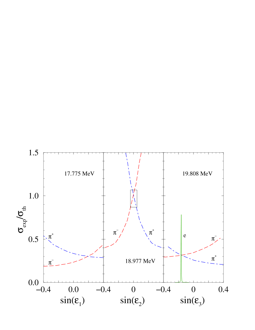
Figure 2: (Color online) Peak height ratios of experiment to theory for $\pi^{\pm}$ scattering to the three $4^{-}$ states in ¹⁶O as functions of isospin mixing.

With that interaction strength we then evaluated the $\pi^{\pm}$ cross sections from excitation of the other (dominantly isoscalar) $4^{-}$ states, ascertaining the normalization scales required to fit the data and allowing variation in isospin mixing. The variation of the peak height ratios $\sigma_{exp}/\sigma_{th}$ so obtained are shown in Fig. 2 as functions of the sines of the coupling angles $\epsilon_{i}$. Such reflects the amount of isospin mixing one might expect for each of the three states. A variation of the peak cross section ratio found with the scattering of electrons exciting the 19.808 MeV state is also shown as it also emphasizes the isospin mixing expectation for that state. The variation with isospin mixing of the $\pi^{+}$ scattering cross section peak ratio is markedly different to that for $\pi^{-}$ scattering in all three cases and those variations are quite sharp. Where the two projectile variations cross then indicates the amount of isospin mixing to be expected. With the 19.808 MeV excitation, the electron scattering data are only known as upper bounds and so using those (small) values gives a very sharp change when isospin mixing in that dominantly isoscalar state is used to calculate the relevant $M4$ transverse electric form factor. That variation confirms well the suggested isospin admixing with $\sin(\epsilon_{3})=-0.17$. Thus we assumed, initially as least, that the isospin mixing in the three $4^{-}$ states of ¹⁶O to be $\sin(\epsilon_{1})=0.2$ for the 17.775 MeV state, $\sin(\epsilon_{2})=0$ for the 18.977 MeV state, and $\sin(\epsilon_{3})=-0.17$ for the 19.808 MeV state.

Holtkamp et al. Holtkamp et al. (1980) quote a ratio of $\pi^{\pm}$ summed yields for excitation of the 18.977 MeV state as $0.964\pm 0.08$ so allowing some small amount of isospin mixing. A conservative estimate is shown by the width of the dotted box around the cross over point in the middle panel of Fig. 2.

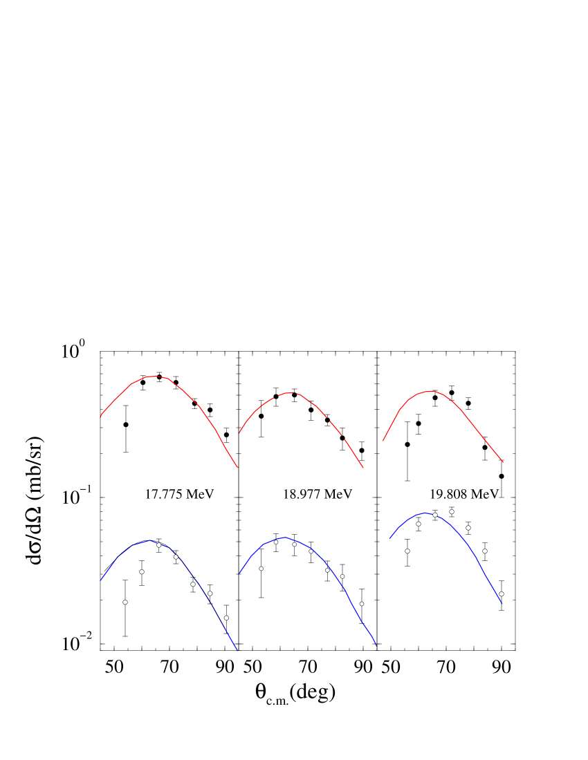
Figure 3: (Color online) Differential cross sections for $\pi^{\pm}$ scattering to the three $4^{-}$ states in ¹⁶O with fits requiring overall scale factors as given in the text.

In Fig. 3, the differential cross sections measured Holtkamp et al. (1980) for the inelastic scattering of pions from ¹⁶O and leading to the $4^{-}$ states are compared with DWIA calculated results. The interaction operator strength was set by assuming the 18.977 MeV state to be described by the pure isovector basis state $\left|a\right>$ of Eq. (9). That is consistent also with previous DWIA analyses Carr et al. (1983) of the same data as well as of cross sections from the excitation of “stretched” $6^{-}$ states in ²⁸Si. The fits to the data from the other states required scales of 0.3 and 0.34, for the 17.775 and 19.808 MeV states respectively when the isospin admixing suggested by the peak height ratio study described above. That isospin mixing was particularly crucial since the relative peak height ratios of the $\pi^{+}$ and $\pi^{-}$ vary so markedly with the mixing. However, the shapes of the cross sections calculated for the dominantly isoscalar states do not match the data as well as they could. Indeed a previous analysis Carr et al. (1983) used spin transition densities extracted from electron scattering which resulted in better cross sections shapes than we show. But such improvements are not central to this composite data study and, in any event, would require a better specification of the $\pi^{\pm}N$ $g$-matrices including allowance of the $T=\frac{1}{2}$ transition amplitudes; components found to be of some import, despite $\Delta$ dominance, in studies of $\pi^{\pm}$ asymmetries in cross sections for excitation of the $\frac{9}{2}^{+}$ state in ¹³C Amos and Morrison (1981). Furthermore, any such refinement has not been made since there are also vagaries with the phenomenology involved in the calculations.

IV.2 Electron and proton elastic scattering from ¹⁶O

The charge density shown in Fig. 1, is tested by using it in evaluations of the longitudinal form factor for elastic electron scattering.

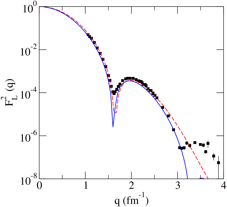
Figure 4: (Color online) The longitudinal form factor from electron elastic scattering on ¹⁶O. The data Sick and McCarthy (1970) are compared with the results of calculations made using harmonic oscillator ($b=1.7$ fm) wave functions (dashed curve) and with the set of WS functions (solid curve) defined in the text.

The results of using harmonic oscillators ($b=1.7$ fm) and WS functions are compared with the data Sick and McCarthy (1970) in Fig. 4. The data (filled squares) show that the oscillator (dashed curve) is a good result to $2.5$ fm^-1 while the WS result (solid curve does as well to the second minimum in data at 3 fm^-1. We note that a much better fit to these data above 3 fm^-1 has been found by Mihaila and Heisenberg Mihaila and Heisenberg (2000) by using an $\exp(S)$ coupled-cluster expansion approach. But to achieve those remarkable results necessitated use of an effective 50$\hbar\omega$ space, two-body currents, and Coulomb distortion; things not included in the simple approach we have taken since our purpose is to correlate major effects in scattering of different probes with analyses of data for which momentum transfer values are less than $\sim 3$ fm^-1.

A further test of the propriety of the structure assumed for the ground state is to use that in analyses of the elastic scattering of protons from ¹⁶O. Those we have made using the $g$-folding approach Amos et al. (2000) that has proved quite successful in recent years. Details of the approach are given in the review Amos et al. (2000) as are details of the Melbourne effective $NN$ interaction that is actually folded with the spectroscopy.

We consider proton scattering at 200 MeV first since past studies Amos et al. (2000) of data from many nuclei gave great confidence that the effective $NN$ interaction at that energy was good, and that the method of analysis was appropriate. In Fig. 5, 200 MeV data Seifert et al. (1993) from ¹⁶O (filled circles) are compared with the results (solid curves) found using the $g$-folding method with the appropriate (200 MeV) effective $NN$ interaction, WS bound state functions, and (ground state) OBDME from the complete $(0+2)\hbar\omega$ shell model. These predictions are in very good agreement with that data and especially

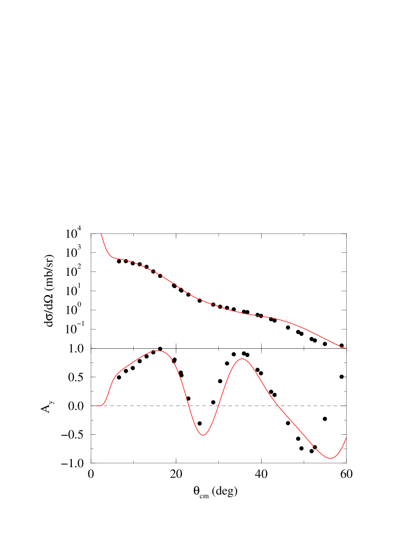
Figure 5: (Color online) Differential Cross section (top) and analyzing power (bottom) for the elastic scattering of 200 MeV protons from ¹⁶O.

the good description of the analyzing power in particular suggests that the ground state spectroscopy we have chosen is realistic.

Using that spectroscopy and simply changing the effective interaction to that appropriate for 135 MeV protons lead then to the results shown in Fig. 6. Therein, the elastic scattering cross sections of 135 MeV protons from ¹⁶O as a ratio to Rutherford scattering are compared with data Amos et al. (1984).

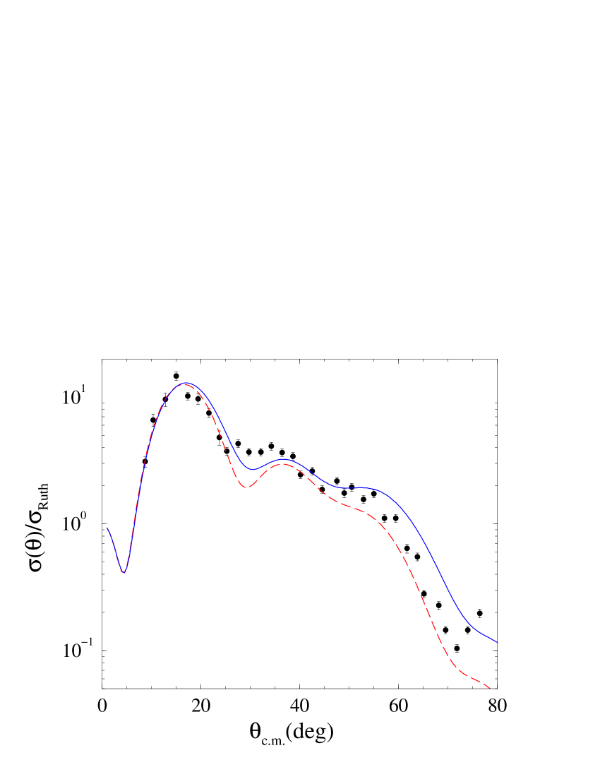
Figure 6: (Color online) Ratio to Rutherford cross sections for the elastic scattering of 135 MeV protons from ¹⁶O. The solid and dashed curves display the results found using WS and oscillator bound state wave functions respectively.

The WS folding result is displayed by the solid curve while the dashed curve portrays that found by using the oscillator functions instead. There are some differences between these results but the WS result is preferred since the cross section forward of 60^∘ is the most significant as a test of the model.

IV.3 $M4$ form factors from inelastic electron scattering

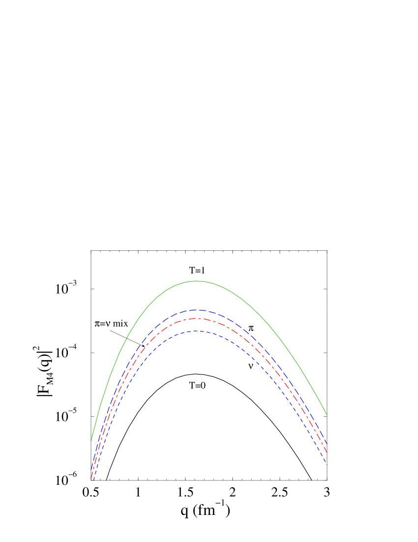
Figure 7: (Color online) $M4$ form factors from electron scattering to the pure isospin “stretched” states of Eq. (9).

The electron scattering data for excitation of the 17.775 and 18.977 MeV states are well defined but only a weak upper limit is known for the $M4$ form factor from excitation of the 19.808 MeV state. As shown earlier, the latter quite strongly confirms the degree of isospin mixing in that state. First we consider the form factors and the separate proton and neutron components that arise when excitations of the pure isospin basis states are considered. The results displayed in Fig. 7 were generated using WS wave functions. The separate proton ($\pi$) and neutron ($\nu$) results are shown by the long and short dashed lines respectively. The dot-dashed line is the pure proton (and neutron) form factor one finds by adjusting the weight values to get identical proton and neutron amplitudes. Clearly the underlying amplitudes interfere constructively and destructively respectively to yield the isovector and isoscalar excitation results. By small weightings, magnitude equal proton and neutron amplitudes can be found and that defines the isospin mixing required to give nett vanishing form factors under conditions of destructive interference. That occurs essentially with the excitation of the 19.808 MeV state. Likewise finite results for the $M4$ form factors from excitation of the other two actual states can be found by such mixing. However, in those cases, there is also configuration mixing to be considered. By selecting the isospin admixtures as suggested from the pion scattering results, the $M4$ form factors from excitation of the 17.775 and 18.977 MeV states by electron scattering are those shown in Fig. 8. The dashed curves are those obtained using oscillator functions whilst those found on using WS functions are displayed by the solid curves. Both sets of calculations required the scalings (down) from the values found assuming that there was no spreading of particle-hole strength over other $4^{-}$ states in the spectrum. The results are in reasonable agreement with those made previously Hyde-Wright et al. (1987) in which oscillator wave functions with oscillator lengths of 1.58 fm were used to improve the comparison of calculated results with the data. As we have used a larger oscillator length, our form factors are more sharply peaked but, as evident, they are consistent with results found using the WS functions and with the elastic scattering data.

Specifically isospin mixing has been taken into account with the analysis of the 17.775 MeV excitation with the mixing angle, $\sin(\epsilon_{1})=0.2$, while the 18.977 MeV transition was taken as a pure isovector excitation.

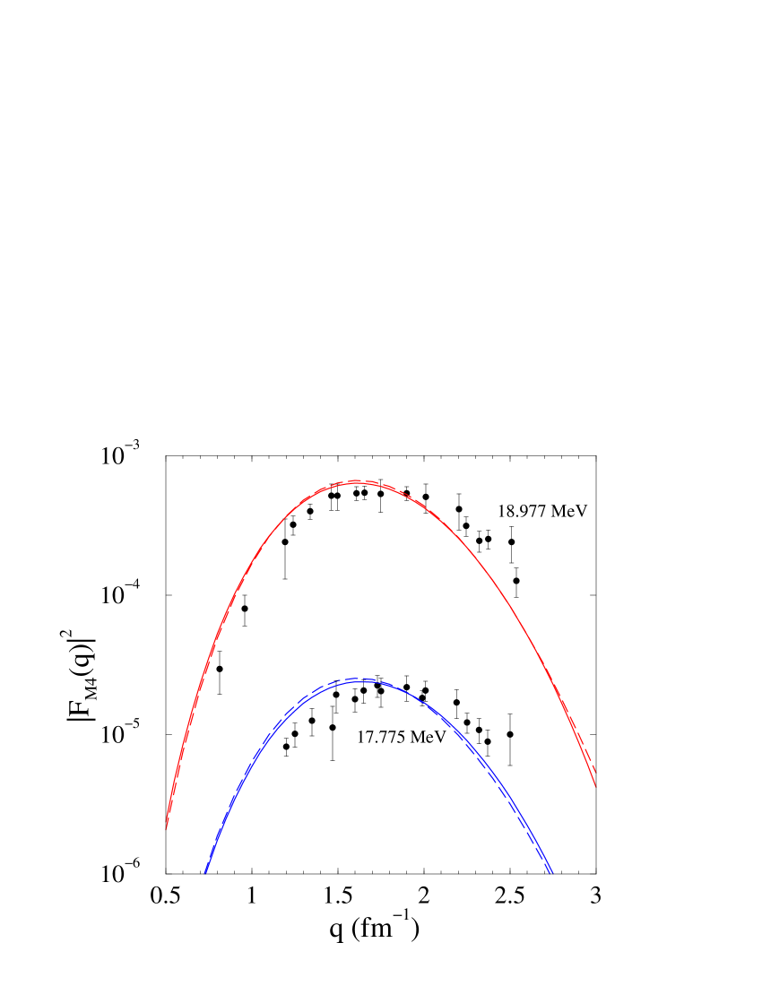
Figure 8: (Color online) $M4$ form factors from electron scattering to the 18.977 MeV and to the 17.775 MeV $4^{-}$ states in ¹⁶O.

But a small isoscalar admixture in this does not vary the peak magnitude markedly. Thus the pure isovector characterization suggested by the pion scattering is neither abrogated nor totally supported by these results. However, they do identify an overall normalization for the state of $N_{2}=0.7$. In contrast, the calculated form factor for the (dominantly isoscalar) 17.775 MeV transition varies noticeably in magnitude with isospin admixture and using the amount selected from the $\pi^{\pm}$ scattering data analyses requires a normalization $N_{1}=0.36$ when harmonic oscillators are taken as the bound state functions. But the dominantly isoscalar transition result arises from an adjustment to the amount of destructive interference between the proton and neutron $M4$ amplitudes. Such makes assessment of the configuration mixing effects difficult. We place more reliability in the proton inelastic scattering results that we discuss next, especially since the separate (bound) proton and neutron amplitudes constructively interfere to define the cross sections.

IV.4 Proton scattering leading to the $4^{-}$ states in ¹⁶O

In this subsection, we present the results of analyses of 135 MeV inelastic scattering data Henderson et al. (1979), of 135 MeV ($p,n$) data (to the IAS $4^{-}$ state in ¹⁶F) and of the analyzing power measured in that experiment Madey et al. (1982). The latter is of particular interest in that spin observables usually are quite sensitive to details in the calculations. As we shall see, at 135 MeV, the charge exchange data track the inelastic proton scattering cross section quite well with but a scale factor of 2. That should be so if the state in ¹⁶F is a true IAS of the 18.977 MeV isovector state in ¹⁶O.

All calculations have been made using a DWA approach with the distorted waves being those generated from evaluation of the elastic scattering of 135 MeV protons from ¹⁶O and the transition operator being the same effective interaction that we used in the $g$-folding solution of that elastic scattering.

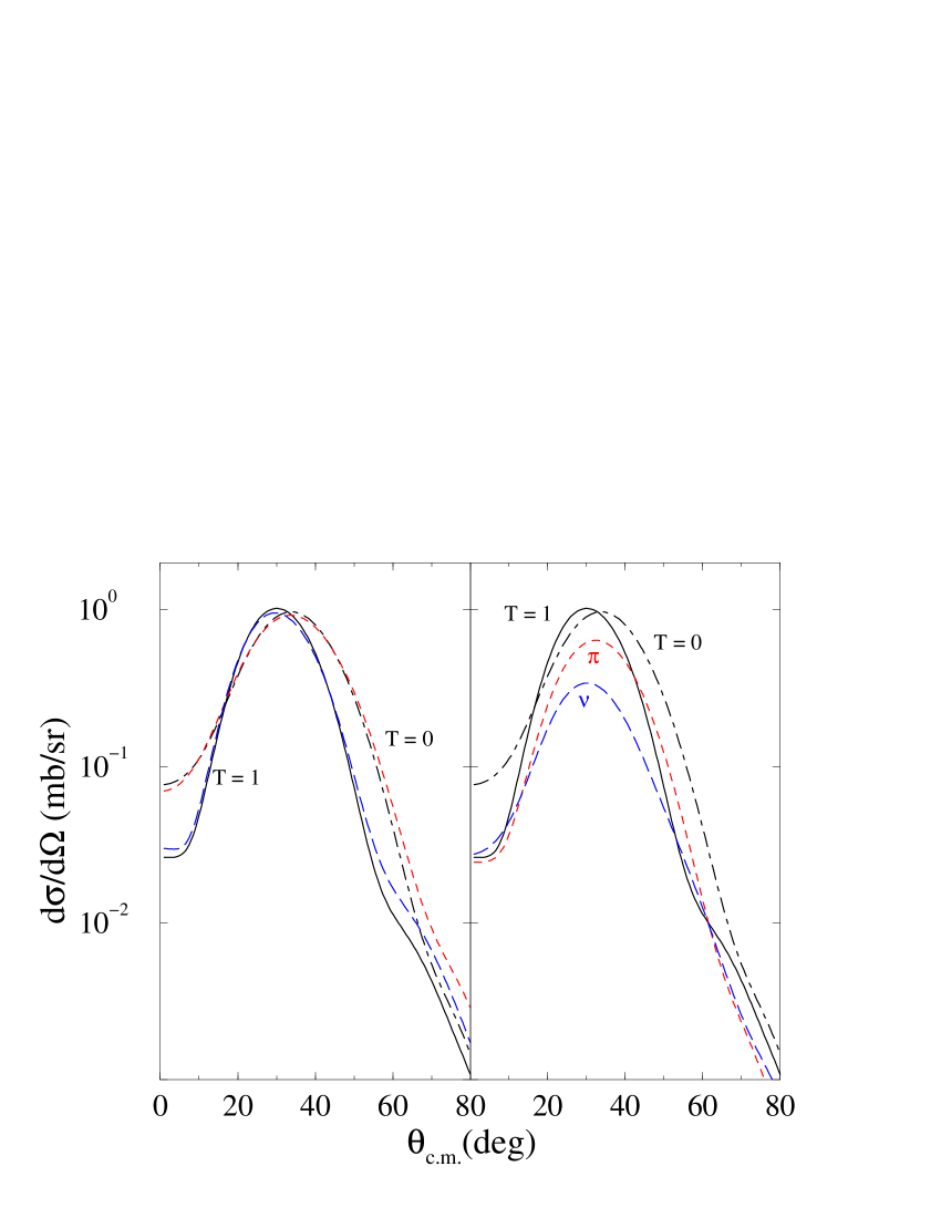
Figure 9: (Color online) Differential cross sections for the inelastic scattering of 135 MeV protons from ¹⁶O exciting pure isospin “stretched” $4^{-}$ states.

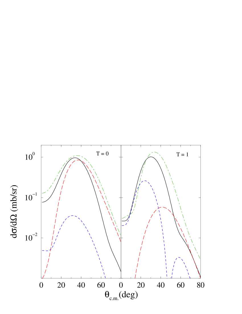
Figure 10: (Color online) Differential cross sections for the inelastic scattering of 135 MeV protons from ¹⁶O exciting pure isospin “stretched” $4^{-}$ states and the contributions from different components of the transition operator.

First consider cross sections from the excitation of the pure isoscalar and isovector “stretched” $4^{-}$ states. The results of those DWA calculations are displayed in Fig 9. The isovector and isoscalar results are those labeled by $T=1$ and $T=0$ in both panels of the figure. Harmonic oscillator bound state functions with $b=1.7$ fm were used to get most of those results. Shown in the right hand panel are the pure proton ($\pi$) and pure neutron ($\nu$) excitation cross sections. They are noticeably different and the interferences between them to effect the pure isoscalar and pure isovector excitations result in cross sections that have similar magnitude but different peak positions. This is a quite different phenomenon than is evident with the electron scattering form factors for which the isoscalar and isovector form factors have so vastly different magnitudes. In the left panel, the harmonic oscillator results (solid curve for $T=1$, dot-dashed curve for $T=0$) are compared with those obtained using the WS bound state functions (long dash curve for $T=1$, short dash curve for $T=0$). Clearly the differences are very minor until larger momentum transfer values are involved.

The proton scattering results are determined by the nature of the transition operator and the characteristics of it that most influence the results are revealed in Fig. 10. The cross sections from excitation of the pure $4^{-}$ isoscalar (left) and isovector (right) states and the contributions from the central parts of the transition operator (dashed curves), from the two-nucleon spin-orbit (${\bf L\cdot S}$) components (long dashed curves) and from the tensor (${\bf S}_{12}$) components (dot-dashed curves) are shown. Clearly the dominant component in these $4^{-}$ excitations is that of the tensor force while the ${\bf L\cdot S}$ terms are more important for the isoscalar than for the isovector transitions. The interference between the tensor and ${\bf L\cdot S}$ contributions in the isoscalar transition is the cause of the shape difference of the total result from that for the isovector excitation.

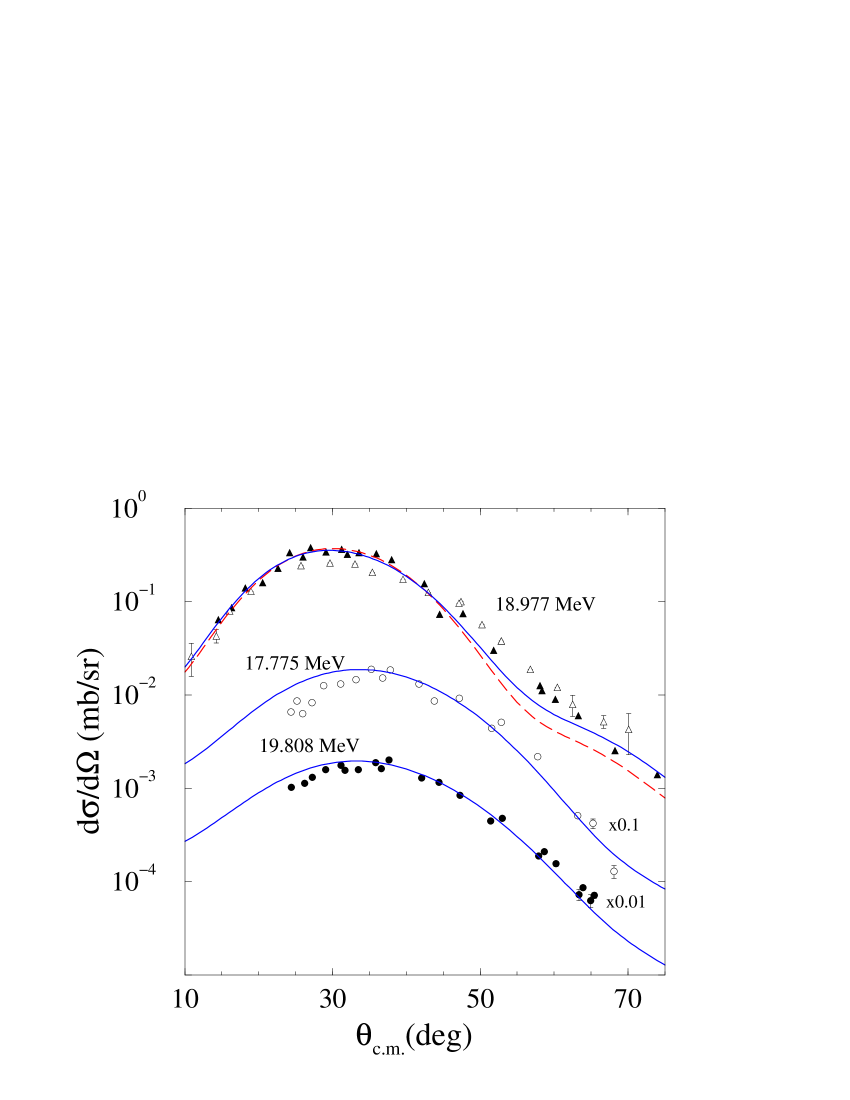
Figure 11: (Color online) Differential cross sections for the inelastic scattering of 135 MeV protons from ¹⁶O exciting the three $4^{-}$ states. The 17.775 and 19.808 MeV data and results have been shifted by 0.1 and 0.01 in scale for visualization. The charge exchange (IAS) ($p,n$) cross section data divided by 2 are shown by the open triangles.

The complete results for the 135 MeV proton scattering cross sections to the actual $4^{-}$ states in ¹⁶O are shown in comparison with data in Fig. 11. The isospin mixing as suggested by the analyses of the pion and electron scattering data have been used and the results scaled to fit; the scalings being identified as the configuration mixing weights. The solid lines are the results of DWA calculations made using the WS bound state functions while the dashed curve displays the result for the 18.977 MeV excitation found using harmonic oscillators. Clearly the shapes of the measured data are well reproduced with the distinguishing features of the dominantly isovector and isoscalar transitions being most evident. The scales, $N_{i}$, of Eq. (12) that were required to obtain these matches to the cross-section magnitudes were $N_{1}=0.42$, $N_{2}=0.62$, and $N_{3}=0.49$.

Finally we consider the analyzing power results to compare with the data taken in a 135 MeV charge exchange experiment Madey et al. (1982). The results are presented in Fig. 12.

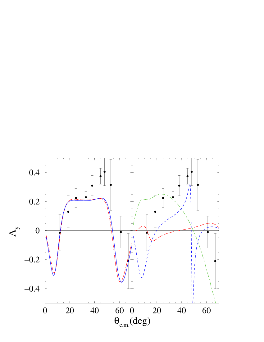
Figure 12: (Color online) Analyzing power for the charge exchange reaction of 135 MeV protons from ¹⁶O exciting the $4^{-}$ IAS state at 6.41 MeV.

In the left panel the total result as found using the WS bound state functions is displayed by the solid curve while that found using the harmonic oscillators is depicted by the dashed curve. In the right panel, the results found using the separate central (dash), tensor (dot-dash), and two-nucleon spin-orbit (long dash) terms in the transition operator are presented. Note that these component results are normalized against the individual component cross sections they form (see the right panel of Fig. 10) and so their relative importance should be considered with comparison of the component against the total cross section. However, the tensor and spin-orbit amplitudes in particular are needed and their interference is crucial in finding the final total result that matches the data as well as it does.

V Conclusions

The simultaneous analyses of electron, pion, and proton scattering data leading to the 4^- states in ¹⁶O ascertain that the states at 17.775 MeV and 19.808 MeV are dominantly isoscalar having isovector admixtures specified by

$$N_{1}\sin(\epsilon_{1})=0.42\ \sin(11.5^{\circ})\ ,$$ (20)

and

$$N_{3}\sin(\epsilon_{3})=0.49\ \sin(-9.8^{\circ})\ ,$$ (21)

while the 18.977 MeV state is virtually pure isovector in nature with $N_{2}=0.62$ being expected from the proton scattering data analyses. Thus we assess that the fractional exhaustion of the ($0d_{\frac{3}{2}}-0p_{\frac{3}{2}}^{-1};T$) strengths exhausted in these transitions are

$$(0d_{\frac{3}{2}}-0p_{\frac{3}{2}}^{-1};T=0) = \left|0.42\ \cos(11.5^{\circ})\right|^{2}+\left|0.49\ \cos(-9.8^{\circ})\right|^{2}=0.40$$

$$(0d_{\frac{3}{2}}-0p_{\frac{3}{2}}^{-1};T=1) = \left|0.62\right|^{2}+\left|0.42\ \sin(11.5^{\circ})\right|^{2}+\left|0.49\ \sin(-9.8^{\circ})\right|^{2}=0.40\ .$$ (22)

These values are less than one half of what has been assessed in the past from particle transfer data. But as the transfer data assessment is very much phenomenological model calculation dependent, particularly with what overall strength of interaction is chosen in zero-range DWBA calculations, and with a limited model spectroscopy which ascribed $J^{\pi}=2^{-}$ to the state at 17.775 MeV excitation. As this is now known to be a $4^{-}$ state, and there is at least a fourth $4^{-}$ state at 20.5 MeV excitation, we believe our deduced numbers to be the more credible.

Appendix A Normalization of the $\left|4^{-};T_{f}\right>$ states

The normalization constant ${\cal N}$ of the $4^{-};T_{f}$ states follows from

$$1 = \left<4^{-};T_{f}\Bigl{|}4^{-};T_{f}\right>$$ (23)

$$= {\cal N}^{2}\sum(-)^{\left(\frac{1}{2}-\alpha\right)}(-)^{\left(\frac{1}{2}-\alpha^{\prime}\right)}(-)^{\left(\frac{3}{2}-m_{3}\right)}(-)^{\left(\frac{3}{2}-m_{3}^{\prime}\right)}$$

$$\times\left\langle\frac{1}{2}\,\frac{1}{2}\,\alpha\,-\alpha\Bigl{|}T\,0\right\rangle\left\langle\frac{1}{2}\,\frac{1}{2}\,\alpha^{\prime}\,-\alpha^{\prime}\Bigl{|}T\,0\right\rangle\left\langle\frac{3}{2}\,\frac{5}{2}\,m_{3}\,-m_{5}\Bigl{|}4\,-M_{4}\right\rangle\left\langle\frac{3}{2}\,\frac{5}{2}\,m_{3}^{\prime}\,-m_{5}^{\prime}\Bigl{|}4\,-M_{4}\right\rangle$$

$$\times\left\langle 0^{+}\Bigl{|}a_{\frac{3}{2}m_{3}^{\prime}\alpha^{\prime}}^{\dagger}a_{\frac{5}{2}m_{5}^{\prime}\alpha^{\prime}}a_{\frac{5}{2}m_{5}\alpha}^{\dagger}a_{\frac{3}{2}m_{3}\alpha}\Bigr{|}0^{+}\right\rangle\ .$$

The ground state expectation values then reduce as

$$\left\langle 0^{+}\Bigl{|}a_{\frac{3}{2}m_{3}^{\prime}\alpha^{\prime}}^{\dagger}a_{\frac{5}{2}m_{5}^{\prime}\alpha^{\prime}}a_{\frac{5}{2}m_{5}\alpha}^{\dagger}a_{\frac{3}{2}m_{3}\alpha}\Bigr{|}0^{+}\right\rangle = \left\langle 0^{+}\Bigl{|}\left\{\delta_{m_{5}m_{5}^{\prime}}-a_{\frac{5}{2}m_{5}\alpha}^{\dagger}a_{\frac{5}{2}m_{5}^{\prime}\alpha^{\prime}}\right\}a_{\frac{3}{2}m_{3}^{\prime}\alpha^{\prime}}^{\dagger}a_{\frac{3}{2}m_{3}\alpha}\Bigr{|}0^{+}\right\rangle$$ (24)

$$= \delta_{m_{5}^{\prime}m_{5}}\delta_{m_{3}^{\prime}m_{3}}\delta_{\alpha^{\prime}\alpha}\left\{1-\sigma_{\frac{5}{2}\alpha}\right\}\sigma_{\frac{3}{2}\alpha}\ ,$$

where the fractional occupancies (of each orbit) are defined from

$$\left\langle 0^{+}\Bigl{|}a_{jm^{\prime}\alpha^{\prime}}^{\dagger}a_{jm\alpha}\Bigr{|}0^{+}\right\rangle=\delta_{m^{\prime}m}\delta_{\alpha^{\prime}\alpha}\ \sigma_{j\alpha}\ .$$ (25)

In this we assume that every orbit $j,m$ is equally occupied with

$$\sigma_{jx}=\sigma_{jmx}=\frac{1}{2j+1}n_{jx}\ ,$$ (26)

where $n_{jx}$ is the number of nucleons of type $x$ that are contained in the shell $j$ in the target. For a packed shell, as $n_{jx}=(2j+1)$, then $\sigma_{jx}=1$.

Thus

$${\cal N}^{-2} = \sum_{m_{3}m_{5}}\left[\left\langle\frac{3}{2}\,\frac{5}{2}\,m_{3}\,-m_{5}\Bigl{|}4\,-M_{4}\right\rangle\right]^{2}\sum_{\alpha}\left[\left\langle\frac{1}{2}\,\frac{1}{2}\,\alpha\,-\alpha\Bigl{|}T\,0\right\rangle\right]^{2}\left\{1-\sigma_{\frac{5}{2}\alpha}\right\}\sigma_{\frac{3}{2}\alpha}$$ (27)

$$= \sum_{\alpha}\left[\left\langle\frac{1}{2}\,\frac{1}{2}\,\alpha\,-\alpha\Bigl{|}T\,0\right\rangle\right]^{2}\left\{1-\sigma_{\frac{5}{2}\alpha}\right\}\sigma_{\frac{3}{2}\alpha}\;=\;\frac{1}{2}\sum_{\alpha}\left\{1-\sigma_{\frac{5}{2}\alpha}\right\}\sigma_{\frac{3}{2}\alpha}\ ,$$

and then, with charge symmetry assumed, the sum over bound nucleon isospins $\alpha$ gives just a factor of 2 and,

$${\cal N}={\sqrt{2}}\left[\sum_{\alpha}\left\{1-\sigma_{\frac{5}{2}\alpha}\right\}\sigma_{\frac{3}{2}\alpha}\right]^{-\frac{1}{2}}\ \equiv\frac{1}{\sqrt{\left\{1-\sigma_{\frac{5}{2}}\right\}\sigma_{\frac{3}{2}}}}$$ (28)

Appendix B Spectroscopic amplitudes

We consider the general matrix element, from which the spectroscopic amplitudes to be used in DWBA98 code evaluations can be derived, namely

$${\cal M}_{(x,y)}=\left\langle 4^{-};T_{f}\left|\left[a_{j_{2}x}^{\dagger}\otimes{\tilde{a}}_{j_{1}y}\right]^{(I)}_{(M_{4})}\right|0^{+};0\right\rangle\ ,$$ (29)

where now we have

$$\left[a_{j_{2}x}^{\dagger}\otimes{\tilde{a}}_{j_{1}y}\right]^{(I)}_{(N)}=\sum_{m_{1}m_{2}}(-)^{\left(j_{1}-m_{1}\right)}\left\langle j_{1}\,j_{2}\,m_{1}\,-m_{2}\Bigl{|}I\,-N\right\rangle\ a_{j_{2}m_{2}x}^{\dagger}\,a_{j_{1}m_{1}y}$$ (30)

while

$$\left|4^{-};T_{f}\right>={\cal N}\left[a^{\dagger}_{\left(\frac{5}{2},\frac{1}{2}\right)}\times{\tilde{a}}^{\phantom{\dagger}}_{\left(\frac{3}{2},\frac{1}{2}\right)}\right]^{(4,T_{f})}_{(M_{4},0)}\left|0^{+};0\right>\ ,$$ (31)

with normalization as given in Eq. (28).

Notice that the transition operator is coupled only in angular momentum and not in isospin. That is so we find spectroscopic amplitudes for bound proton and bound neutron excitations separately as are required in evaluations of both electron form factors and cross sections initiated by nucleons. Those amplitudes, in fact, are the reduced matrix elements from Eq. (29),

$${\cal M}_{(x,y)}=\frac{1}{3}\left<0\,I\,0\,N\Bigl{|}4\,M_{f}\right>\ \left<4^{-};T_{f}\left\|\left[a_{j_{2}x}^{\dagger}\otimes{\tilde{a}}_{j_{1}y}\right]^{I}\right\|0^{+};0\right>\>=\;\frac{1}{3}\,\delta_{I4}\,\delta_{NM_{f}}\,S_{j_{1}\,j_{2}\,4}^{(x,y)}\ .$$ (32)

Thus, evaluation of the spectroscopic amplitudes for these transitions is made using the inverse of this, namely $S_{j_{1}j_{2}4}^{(x,y)}=3\delta_{I4}\delta_{NM_{f}}{\cal M}_{(x,y)}$.

For inelastic scattering, the nucleon type does not change so the $x=y$ in the above. However to consider charge exchange reactions, for which $x=-y$, we have to revise the specification of the final nuclear state. That transition is to the IAS which relates to the $T=1$ state in ¹⁶O by the action of an extra isospin projection changing operator.

B.1 Inelastic scattering

With $x=y$, the general matrix element expands as

$${\cal M}_{(x)} = \left[\left\{1-\sigma_{\frac{5}{2}}\right\}\sigma_{\frac{3}{2}}\right]^{-\frac{1}{2}}\sum_{m_{3}m_{5}\alpha m_{1}m_{2}}(-)^{\left(\frac{1}{2}-\alpha\right)}\left\langle\frac{1}{2}\,\frac{1}{2}\,\alpha\,-\alpha\Bigl{|}T_{f}\,0\right\rangle$$ (33)

$$\;\;\times(-)^{\left(\frac{3}{2}-m_{3}\right)}\left\langle\frac{3}{2}\,\frac{5}{2}\,m_{3}\,-m_{5}\Bigl{|}4\,-M_{4}\right\rangle\,(-)^{\left(j_{1}-m_{1}\right)}\left\langle j_{1}\,j_{2}\,m_{1}\,-m_{2}\Bigl{|}I\,-N\right\rangle$$

$$\;\;\times\left\langle 0^{+};0\left|a^{\dagger}_{\frac{5}{2}m_{5}\alpha}a_{\frac{3}{2}m_{3}\alpha}a_{j_{2}m_{2}x}^{\dagger}a_{j_{1}m_{1}x}\right|0^{+};0\right\rangle\ .$$

Then using the fractional occupancy representation of the expectation, Eq. (25), this reduces to

$${\cal M}_{(x)} = \sqrt{\left\{1-\sigma_{\frac{5}{2}}\right\}\sigma_{\frac{3}{2}}}\ (-)^{\left(\frac{1}{2}-x\right)}\left<\frac{1}{2}\,\frac{1}{2}\,x\,-x\Bigl{|}T_{f}\,0\right>$$ (34)

$$\times\sum_{m_{1}m_{2}m_{3}m_{5}}\delta_{j_{1}\frac{3}{2}}\delta_{m_{1}m_{3}}\delta_{j_{2}\frac{5}{2}}\delta_{m_{2}m_{5}}\left<j_{1}\,j_{2}\,m_{1}\,-m_{2}\Bigl{|}I\,-N\right>\left<\frac{3}{2}\,\frac{5}{2}\,m_{3}\,-m_{5}\Bigl{|}4\,-M_{f}\right>$$

$$= \sqrt{\left\{1-\sigma_{\frac{5}{2}}\right\}\sigma_{\frac{3}{2}}}\ (-)^{\left(\frac{1}{2}-x\right)}\left<\frac{1}{2}\,\frac{1}{2}\,x\,-x\Bigl{|}T_{f}\,0\right>$$

$$= \sqrt{\left\{1-\sigma_{\frac{5}{2}}\right\}\sigma_{\frac{3}{2}}}\;\frac{1}{\sqrt{2}}\left[\delta_{T_{f}0}+(-)^{\left(\frac{1}{2}-x\right)}\delta_{T_{f}1}\right]\ ,$$

so that, for inelastic scattering,

$$S_{j_{1}j_{2}4}^{(x)}=\delta_{j_{1}\frac{3}{2}}\delta_{j_{2}\frac{5}{2}}\frac{3}{\sqrt{2}}\ \sqrt{\left\{1-\sigma_{\frac{5}{2}}\right\}\sigma_{\frac{3}{2}}}\left[\delta_{T_{f}0}+(-)^{\left(\frac{1}{2}-x\right)}\delta_{T_{f}1}\right]\ .$$ (35)

B.2 Charge exchange to the IAS $4^{-}$ in ¹⁶F

First we need to specify the form that the IAS takes. With $T^{-}=\sum_{jm}a_{jm-\frac{1}{2}}^{\dagger}a_{jm\frac{1}{2}}$ being the operator that changes a neutron to a proton, the $4^{-}$ state in ¹⁶F that is an IAS to the particle-hole model isovector $4^{-}$ state in ¹⁶O has the form

$$\left|4^{-};IAS\right\rangle = \left|4^{-};T_{f}=1,M_{T_{f}}=-1\right\rangle={\cal P}T^{-}\left[a^{\dagger}_{\left(\frac{5}{2}\frac{1}{2}\right)}\otimes{\tilde{a}}_{\left(\frac{3}{2}\frac{1}{2}\right)}\right]^{(4,T_{f}=1)}_{(M_{4},0)}\Bigr{|}0^{+};0\Bigr{>}$$ (36)

$$= {\cal P}\sum_{m,\alpha,m_{3}m_{5}}(-)^{\left(\frac{1}{2}-\alpha\right)}\left<\frac{1}{2}\,\frac{1}{2}\,\alpha\,-\alpha\Bigl{|}T_{f}(=1)\,0\right>(-)^{\left(\frac{1}{2}-m_{3}\right)}\left<\frac{3}{2}\,\frac{5}{2}\,m_{3}\,-m_{5}\Bigl{|}4\,-M_{f}\right>$$

$$\;\;\;\times\ a^{\dagger}_{jm-\frac{1}{2}}a_{jm\frac{1}{2}}a^{\dagger}_{\frac{5}{2}m_{5}\alpha}a_{\frac{3}{2}m_{3}\alpha}\Bigl{|}0^{+};0\Bigr{>}\ ,$$

where $\cal P$ is the normalization. Then, the particle-hole description of the $4^{-}$ states requires

$$a^{\dagger}_{jm-\frac{1}{2}}a_{jm\frac{1}{2}}a^{\dagger}_{\frac{5}{2}m_{5}\alpha}a_{\frac{3}{2}m_{3}\alpha}\Bigl{|}0^{+};0\Bigr{>}\equiv\delta_{\alpha,\frac{1}{2}}\delta_{j,\frac{5}{2}}\delta_{mm_{5}}a^{\dagger}_{\frac{5}{2}m_{5}-\frac{1}{2}}a_{\frac{3}{2}m_{3}\frac{1}{2}}\left[1-a^{\dagger}_{\frac{5}{2},m_{5}\frac{1}{2}}a_{\frac{5}{2}m_{5}\frac{1}{2}}\right]\Bigl{|}0^{+};0\Bigr{>}\ ,$$ (37)

and the isospin terms are simply

$$\delta_{\alpha\frac{1}{2}}\ (-)^{\left(\frac{1}{2}-\alpha\right)}\left<\frac{1}{2}\,\frac{1}{2}\,\alpha\,-\alpha\Bigl{|}T_{f}(=1)\;0\right>=\frac{1}{\sqrt{2}}\ ,$$ (38)

the IAS state becomes

$$\Bigl{|}4^{-};IAS\Bigr{>} = {\cal P}\frac{1}{\sqrt{2}}\sum_{m_{3}m_{5}}(-)^{\left(\frac{1}{2}-m_{3}\right)}\left<\frac{3}{2}\,\frac{5}{2}\,m_{3}\,-m_{5}\Bigl{|}4\,-M_{f}\right>$$ (39)

$$\;\;\;\times a^{\dagger}_{\frac{5}{2}m_{5}-\frac{1}{2}}a_{\frac{3}{2}m_{3}\frac{1}{2}}\left[1-a^{\dagger}_{\frac{5}{2},m_{5}\frac{1}{2}}a_{\frac{5}{2}m_{5}\frac{1}{2}}\right]\Bigl{|}0^{+};0\Bigr{>}\ .$$

Normalization then defines $\cal P$ since, with $a_{jmx}^{\dagger}a_{jmx}$ is the ’$x$’ nucleon number operator leading to $\sigma_{jx}$

$$1 = \left<4^{-};IAS\bigl{|}4^{-};IAS\right>$$ (40)

$$= {\cal P}^{2}\frac{1}{2}\sum_{m_{3}m_{5}m_{3}^{\prime}m_{5}^{\prime}}(-)^{\left(\frac{1}{2}-m_{3}^{\prime}\right)}\left<\frac{3}{2}\,\frac{5}{2}\,m_{3}^{\prime}\,-m_{5}^{\prime}\Bigl{|}4\,-M_{f}\right>(-)^{\left(\frac{1}{2}-m_{3}\right)}\left<\frac{3}{2}\,\frac{5}{2}\,m_{3}\,-m_{5}\Bigl{|}4\,-M_{f}\right>$$

$$\times\left<0^{+};0\left|\left[1-\sigma_{\frac{5}{2}\frac{1}{2}}\right]a^{\dagger}_{\frac{3}{2}m_{3}^{\prime}\frac{1}{2}}a_{\frac{5}{2}m_{5}^{\prime}-\frac{1}{2}}a^{\dagger}_{\frac{5}{2}m_{5}-\frac{1}{2}}a_{\frac{3}{2}m_{3}\frac{1}{2}}\left[1-\sigma_{\frac{5}{2}\frac{1}{2}}\right]\right|0^{+};0\right>$$

$$= {\cal P}^{2}\frac{1}{2}\left[1-\sigma_{\frac{5}{2}\frac{1}{2}}\right]^{2}\left[1-\sigma_{\frac{5}{2}-\frac{1}{2}}\right]\ \sigma_{\frac{3}{2}\frac{1}{2}}$$

so that on inversion and with identical fractional occupancies for proton and neutron shells,

$${\cal P}=\sqrt{2\Bigl{/}\left\{\left[1-\sigma_{\frac{5}{2}}\right]^{3}\sigma_{\frac{3}{2}}\right\}}.$$ (41)

The spectroscopic amplitude follows then by using Eqs. (39) and (41) in forming

$$S_{j_{1}j_{2}I}^{-\frac{1}{2}\frac{1}{2}} = 3\left<4^{-};IAS\left|\left[a_{j_{2}-\frac{1}{2}}\otimes{\tilde{a}}_{j_{1}\frac{1}{2}}\right]^{I}_{N}\right|0;0\right>$$ (42)

$$= \frac{3}{\sqrt{2}}\left[\frac{2}{\left[1-\sigma_{\frac{5}{2}}\right]^{3}\sigma_{\frac{3}{2}}}\right]^{\frac{1}{2}}$$

$$\times\sum_{m_{1}m_{2}}(-)^{(j_{1}-m_{1})}\left<j_{1}\,j_{2}\,m_{1}\,-m_{2}\Bigl{|}I\,-N\right>\,(-)^{(\frac{3}{2}-m_{3})}\left<\frac{3}{2}\,\frac{5}{2}\,m_{3}\,-m_{5}|4\,-M_{f}\right>$$

$$\;\;\;\times\left<0^{+};0\left|\left[1-\sigma_{\frac{5}{2}}\right]a^{\dagger}_{\frac{3}{2}m_{3}\frac{1}{2}}\ a_{\frac{5}{2}m_{5}-\frac{1}{2}}a^{\dagger}_{j_{2}m_{2}-\frac{1}{2}}a_{j_{1}m_{1}\frac{1}{2}}\right|0^{+};0\right>$$

$$= 3\frac{1}{\sqrt{\left[1-\sigma_{\frac{5}{2}}\right]^{3}\sigma_{\frac{3}{2}}}}\left[1-\sigma_{\frac{5}{2}}\right]^{2}\sigma_{\frac{3}{2}}\;=\;3\sqrt{\left[1-\sigma_{\frac{5}{2}}\right]\sigma_{\frac{3}{2}}}\;(\delta_{T_{f}1})\ .$$

This is $\sqrt{2}$ times the value found for inelastic scattering as given in Eq. (35) and so the charge exchange cross section should be twice that for inelastic scattering to the IAS.

References

- Uberall (1971) H. Uberall, Electron Scattering from Complex Nuclei (Academic Press, New York, 1971).
- Friar and Fallieros (1984) J. L. Friar and S. Fallieros, Phys. Rev. C 29, 1645 (1984).
- Friar and Fallieros (1985) J. L. Friar and S. Fallieros, Phys. Rev. C 31, 2027 (1985).
- Karataglidis et al. (1995a) S. Karataglidis, P. Halse, and K. Amos, Phys. Rev. C 51, 2494 (1995a).
- Amos et al. (2000) K. Amos, P. J. Dortmans, H. V. von Geramb, S. Karataglidis, and J. Raynal, Adv. in Nucl. Phys. 25, 275 (2000).
- Hyde-Wright et al. (1987) C. E. Hyde-Wright et al., Phys. Rev. C 35, 880 (1987).
- Clausen et al. (1988) B. L. Clausen, R. J. Peterson, and R. A. Lindgren, Phys. Rev. C 38, 589 (1988).
- Lagoyannis et al. (2001) A. Lagoyannis et al., Phys. Lett. B518, 27 (2001).
- Karataglidis et al. (2002) S. Karataglidis, K. Amos, B. A. Brown, and P. K. Deb, Phys. Rev. C 65, 044306 (2002).
- Dupuis et al. (2005) M. Dupuis, S. Karataglidis, E. Bauge, J. P. Delaroche, and D. Gogny (2005), nucl-th/0504013.
- Pearlman (1993) S. Pearlman, ENDF/HE-VI Mat-625 (1993), BNL-48035.
- Anderson et al. (1979) B. D. Anderson et al., IUCF annual report (1979), p. 29.
- Madey et al. (1982) R. Madey et al., Phys. Rev. C 25, 1715 (1982).
- Ohnuma et al. (1982) H. Ohnuma et al., Phys. Lett. 112B, 206 (1982).
- Holtkamp et al. (1980) D. B. Holtkamp et al., Phys. Rev. Letts. 45, 420 (1980).
- Millener and Kurath (1975) D. J. Millener and D. Kurath, Nucl. Phys. A255, 315 (1975), and references cited therein.
- Smith et al. (1978) R. Smith, J. Morton, I. Morrison, and K. Amos, Aust. J. Phys. 31, 1 (1978).
- Mairle et al. (1978) G. Mairle, G. J. Wagner, P. Doll, K. T.Knoepfle, and H. Breuer, Nucl. Phys. A299, 39 (1978).
- Karataglidis et al. (1995b) S. Karataglidis, P. J. Dortmans, K. Amos, and R. de Swiniarski, Phys. Rev. C 53, 838 (1995b).
- Barker et al. (1981) F. Barker, R. Smith, I. Morrison, and K. Amos, J. Phys. G7, 657 (1981).
- Petrovich and Love (1983) F. Petrovich and W. G. Love, Nucl. Phys. A354, 499 (1983).
- Stricker et al. (1979) K. Stricker, H. McManus, and J. A. Carr, Phys. Rev. C 19, 929 (1979).
- Mihaila and Heisenberg (2000) B. Mihaila and J. H. Heisenberg, Phys. Rev. C 61, 54309 (2000).
- Sick and McCarthy (1970) I. Sick and J. S. McCarthy, Nucl. Phys. A150, 631 (1970).
- Raynal (1998) J. Raynal (1998), computer program DWBA98, NEA 1209/05.
- Carr et al. (1983) J. A. Carr, F. Petrovich, D. Halderson, D. B. Holtkamp, and W. B. Cottingame, Phys. Rev. C 27, 1636 (1983).
- Amos and Morrison (1981) K. Amos and I. Morrison, Phys. Rev. C 23, 1679 (1981).
- Seifert et al. (1993) H. Seifert et al., Phys. Rev. C 47, 1615 (1993).
- Amos et al. (1984) K. Amos et al., Nucl. Phys. A413, 255 (1984).
- Henderson et al. (1979) R. S. Henderson et al., Aust. J. Phys. 32, 411 (1979).