Spectroscopy of Medium to Heavy Single $\Lambda$-Hypernuclei

Abstract

We develop a method for calculating the doublet splittings of select ground-state single $\Lambda$-hypernuclei. This hypernuclear spectroscopy is conducted by supplementing the self-consistent single-particle equations with an effective interaction, which follows directly from the underlying lagrangian, to simulate the residual particle-hole interaction. Our previous investigation, performed using only the leading-order contributions to the particle-hole interaction, was inadequate. In the present work, this method is improved upon by increasing the level of truncation in the residual interaction to include gradient couplings to the neutral vector meson, and thereby incorporating the tensor force into the calculation (which is known to play a crucial role in these systems). As a result, we obtain a realistic description of the effect of the tensor couplings on the doublet orderings and splittings.

1 Introduction

In the Kohn–Sham framework, the nuclear many-body system is reduced to a set of single-particle equations with classical fields [1, 2, 3]. This framework allows one to reproduce the exact ground-state energy, scalar and vector densities, and chemical potential, provided that the mean-field energy functional is accurately calibrated. In some cases, however, the single-particle levels are actually weighted averages of multiple states [4]. To illustrate this point, consider the ground-state of ${}^{32}_{15}$P₁₇, which has the configuration $(2{\mathrm{s}}_{1/2})_{\mathrm{p}}(1{\mathrm{d}}_{3/2})_{\mathrm{n}}$. The angular momenta of the valence proton and neutron couple; therefore, the calculated Kohn–Sham ground-state is actually a doublet. To determine the true level orderings and splittings, one can supplement the Kohn–Sham equations with a Tamm-Dancoff Approximation (TDA) analysis of the particle-hole states. The particle-hole matrix elements are sums of two-body Dirac matrix elements, and the particle-hole interaction is determined by the underlying effective field theory. If retardation is neglected, the interaction is given by (Yukawa) meson-exchange potentials (with appropriate spin-isospin operators). This approach has been used to study ordinary nuclei [5] and single $\Lambda$-hypernuclei [6]. The case of single $\Lambda$-hypernuclei is particularly interesting as no single isovector coupling is allowed, and there are no exchange contributions, since the $\Lambda$ and the nucleon are distinguishable. This will allow us to focus on isoscalar exchange in the effective interaction.

There are no free parameters in this TDA analysis. As a result, there are only three possible ways to adjust this method: vary the level of truncation in the underlying lagrangian, introduce additional degrees of freedom, or include higher-order contributions in the particle-hole interaction. It is of interest to investigate the effect of these modifications on the accuracy of this approach, particularly the inclusion of higher-order terms involving gradient couplings. We have applied this specific improvement to calculations of ground-state, $\Lambda$-particle–nucleon-hole splittings in single $\Lambda$-hypernuclei, such as ${}^{16}_{\Lambda}$O. The higher-order terms that are of interest here are those involving the tensor coupling to the neutral vector meson; these terms incorporate the tensor force into the calculation, which is known to play a crucial role in these systems [7, 8] and does not enter in leading-order contributions [6].

In recent years, a number of new avenues have opened to study hypernuclei with increased accuracy. Of particular interest to this work are $\gamma$-ray coincidence and $(e,e^{\prime}K^{+})$ experiments. Recent $\gamma$-ray experiments have measured the fine structure of a number of light hypernuclei [9, 10], including the measurement of the ground-state particle-hole splitting in ${}_{\Lambda}^{16}$O. High precision $(e,e^{\prime}K^{+})$ experiments have measured, or are set to measure, a number of similar states in light hypernuclei [11, 12], including the ground-states of ${}_{\Lambda}^{12}$B and ${}_{\Lambda}^{16}$N. Unfortunately, most of the states that have been measured with these techniques thus far lie below the range of $A$ accessible to the Kohn-Sham approach used in this work; therefore, the experimental constraints on heavier hypernuclei are confined to upper bounds provided by $\left(\pi^{+},K^{+}\right)$ reactions [13, 14, 15]. It is this region of medium to heavy single $\Lambda$-hypernuclei that this work seeks to investigate.

A number of recent calculations have tackled this problem. Shell model calculations in p-shell hypernuclei were conducted using two-body matrix elements, accurately describing the known data [7, 8]. The influence of zero-range effective $\Lambda$NN interactions on p-shell hypernuclei has also been investigated [16]. Another model of interest uses strangeness changing response functions to calculate the spectra of ${}^{16}_{Y}$O and ${}^{40}_{Y}$Ca; the resulting ground-state particle-hole splittings are small [17]. The spectra of ${}_{\Lambda}^{16}$O has also been calculated from a folded diagram method using realistic hyperon-nucleon potentials [18].

In Section 2, we develop a method to calculate the particle-hole matrix elements of interest here. We then present the results of this analysis and make some conclusions in Section 3.

2 $\mathbf{s_{1/2}}$-doublets

Consider nuclei like ${}_{\Lambda}^{16}$O; the ground-states of such systems are, in fact, particle-hole states. One process by which nuclei of this type are created is the reaction $\left(\pi^{+},K^{+}\right)$ on target nuclei with closed proton and neutron shells [13, 14, 15]. During the course of this reaction a neutron is converted into a $\Lambda$. As a result, a neutron hole is also created which, for the ground-state, inhabits the outermost neutron shell. The angular momentum of the $\Lambda$ and the neutron hole couple to form a multiplet. However, due to the fact that in the ground-state the $\Lambda$ occupies the $1\mathrm{s}_{1/2}$ shell, there are only two states in these multiplets. It is these configurations that we refer to as s_1/2-doublets. The reaction $(e,e^{\prime}K^{+})$ is another process used to create nuclei of this type [11, 12]. This process differs in that a proton hole is created here and that greater resolution is possible.

In order to calculate the size of these splittings, we must first construct an effective interaction to model these systems. The procedure we follow here is similar to the method developed by Machleidt and others [19]. In this scheme, the effective NN interaction is represented by the exchange of mesons; then, a hierarchy of Feynman diagrams depicting all the possible interactions is developed to reproduce the NN interaction. The contribution for a given diagram is just the product of the vertex contributions and the meson propagator, or

$$V(q_{\mu})=\left(\overline{U}_{\alpha}\Gamma_{1}U_{\alpha}\right)D(q_{\mu})\left(\overline{U}_{\alpha^{\prime}}\Gamma_{2}U_{\alpha^{\prime}}\right)$$ (1)

where $U_{\alpha}$ are the Dirac free fields, $D(q_{\mu})$ is the meson propagator, and the vertex factors, $\Gamma_{1}$ and $\Gamma_{2}$, are taken directly from the underlying effective lagrangian through the relation

$$\delta L_{i}=i\overline{\psi}\Gamma_{i}\psi\phi_{\beta}$$ (2)

where $\phi_{\beta}$ is some meson field operator. However, nuclei are comprised of bound nucleons and not free fields. Therefore, in the present calculation, we improve on this system by replacing the free fields with the Kohn-Sham (or Hartree) wave functions [3]

$$\psi_{\alpha}=\psi_{n\kappa mt}=\frac{1}{r}\left(\begin{array}[]{c}iG_{n\kappa m}(r)\Phi_{\kappa m}(\theta,\phi)\\ -F_{n\kappa m}(r)\Phi_{-\kappa m}(\theta,\phi)\end{array}\right)\zeta_{t}$$ (3)

The contribution for any given diagram now takes the form (following from Eq. (1))

$$V(q_{\mu})=\left(\overline{\psi}_{\alpha}\Gamma_{1}\psi_{\alpha}\right)D(q_{\mu})\left(\overline{\psi}_{\alpha^{\prime}}\Gamma_{2}\psi_{\alpha^{\prime}}\right)$$ (4)

where we now define the effective interaction in momentum space as

$$\overline{V}_{EFT}(q_{\mu})\equiv\Gamma_{1}D(q_{\mu})\Gamma_{2}$$ (5)

and $V_{EFT}(q_{\mu})=\gamma_{4}^{(1)}\gamma_{4}^{(2)}\overline{V}_{EFT}(q_{\mu})$. The meson propagators relevant to this analysis are (here the conventions of [20] are used)

$$\frac{1}{i}\frac{1}{q_{\mu}^{2}+m_{S}^{2}}\;\;\; \;\;\;scalar$$ ;

$$\frac{1}{i}\frac{1}{q_{\mu}^{2}+m_{V}^{2}}\left(\delta_{\mu\nu}+\frac{q_{\mu}q_{\nu}}{m_{V}^{2}}\right)\;\;\; \;\;\;vector$$ ; (6)

The second term in the vector meson propagator vanishes in any calculation due to conservation of the baryon current (as a result, it is henceforth neglected). The relevant nucleon vertex factors are

$$ig_{S}\;\;\; \;\;\;scalar$$ ;

$$-g_{V}\gamma_{\mu}\;\;\; \;\;\;vector$$ ;

$$-\frac{f_{V}g_{V}}{4M}\sigma_{\mu\nu}q_{\mu}\;\;\; \;\;\;vector\;tensor$$ ; (7)

(Note that the $\Lambda$ vertex factors are equivalent to their nucleon counterparts except for the coupling constants [6].) Now a series of diagrams can be written down to represent the NN interaction, each of which will contribute to this effective interaction in the form of Eq. (5). Once a Fourier transform is performed on the effective interaction, it can be used to calculate the two-body matrix elements that govern the particle-hole interactions of interest here.

Now let us return to the case of single $\Lambda$-hypernuclei. The effective $\Lambda$N interaction is determined via the method outlined above and follows directly from our underlying effective lagrangian (see [6]). In this case, no single isovector meson coupling is allowed; as a result, we confine the following discussion to isoscalar, scalar and vector, exchange. As a first approximation, we include only the leading-order contributions arising from contact vertices; this corresponds to simple scalar and neutral vector couplings. To acquire each portion of the effective interaction, we simply take the product of the nucleon vertex factor, the meson propagator, and the $\Lambda$ vertex factor. The simple scalar and neutral vector exchange contributions to the effective interaction take the form

$$\overline{V}_{S}(q_{\mu})=\left(ig_{S}\right)\left(\frac{1}{i}\frac{1}{q_{\mu}^{2}+m_{S}^{2}}\right)\left(ig_{S\Lambda}\right)$$ (8)

$$\overline{V}_{V}(q_{\mu})=\left(-g_{V}\gamma_{\mu}^{(1)}\right)\left(\frac{1}{i}\frac{1}{q_{\mu}^{2}+m_{V}^{2}}\right)\left(-g_{V\Lambda}\gamma_{\mu}^{(2)}\right)$$ (9)

Next we take the Fourier transform of Eqs. (8) and (9), neglecting retardation in the meson propagator (i.e. $q_{4}\rightarrow 0$), and we get

$$\overline{V}_{S}(r_{12})=-\frac{g_{S}g_{S\Lambda}}{4\pi}\frac{e^{-m_{S}r_{12}}}{r_{12}}$$ (10)

$$\overline{V}_{V}(r_{12}) = \frac{g_{V}g_{V\Lambda}}{4\pi}\gamma_{\mu}^{(1)}\gamma_{\mu}^{(2)}\frac{e^{-m_{V}r_{12}}}{r_{12}}$$ (11)

$$= \overline{V}_{V(1)}(r_{12})\gamma_{4}^{(1)}\gamma_{4}^{(2)}+\overline{V}_{V(2)}(r_{12})\gamma_{i}^{(1)}\gamma_{i}^{(2)}$$

where $r_{12}=(r_{1}^{2}+r_{2}^{2}-2r_{1}r_{2}\cos\theta_{12})^{1/2}$. Notice that this corresponds to simple Yukawa couplings to both the scalar and neutral vector mesons. The effective interaction to this order was used in calculations conducted in [6]; unfortunately, it proved inadequate to fully describe the ground-state splittings in single $\Lambda$-hypernuclei. As it turns out, the effective interaction to this order includes only the spin-spin force. However, this neglects the fact that the tensor force is known to play a crucial role in these systems [7, 8]. Therefore, the natural extension of this approach is to include the higher-order contributions involving tensor couplings and thereby incorporate the tensor force into the calculation.

There are three higher-order terms containing gradient vertices (or tensor couplings) of the neutral vector meson; their resulting contributions to the effective interaction are now considered. The contributions from neutral vector meson exchange with a tensor coupling on one vertex to the effective interaction are

$$\overline{V}_{NT}(q_{\mu}) = \left(-\frac{f_{V}g_{V}}{4M}\sigma_{\mu\nu}^{(1)}q_{\mu}\right)\left(\frac{1}{i}\frac{1}{q_{\nu}^{2}+m_{V}^{2}}\right)\left(-g_{V\Lambda}\gamma_{\nu}^{(2)}\right)$$ (12)

$$+\left(\frac{f_{V}g_{V}}{4M}\sigma_{\mu\nu}^{(1)}q_{\nu}\right)\left(\frac{1}{i}\frac{1}{q_{\mu}^{2}+m_{V}^{2}}\right)\left(-g_{V\Lambda}\gamma_{\mu}^{(2)}\right)$$

$$\overline{V}_{\Lambda T}(q_{\mu}) = \left(-g_{V}\gamma_{\mu}^{(1)}\right)\left(\frac{1}{i}\frac{1}{q_{\mu}^{2}+m_{V}^{2}}\right)\left(-\frac{g_{T\Lambda}g_{V}}{4M}\sigma_{\mu\nu}^{(2)}q_{\nu}\right)$$ (13)

$$+\left(-g_{V}\gamma_{\nu}^{(1)}\right)\left(\frac{1}{i}\frac{1}{q_{\nu}^{2}+m_{V}^{2}}\right)\left(\frac{g_{T\Lambda}g_{V}}{4M}\sigma_{\mu\nu}^{(2)}q_{\mu}\right)$$

where the contribution with the tensor coupling on the nucleon ($\Lambda$) vertex is denoted by $\overline{V}_{NT}$ ($\overline{V}_{\Lambda T}$). Notice that two terms arise in both $\overline{V}_{NT}$ and $\overline{V}_{\Lambda T}$ due to the fact that the quantity $V_{\mu\nu}=\partial_{\mu}V_{\nu}-\partial_{\nu}V_{\mu}$ appears in the lagrangian [6]. Now the Fourier transforms of Eqs. (12) and (13), neglecting retardation in the meson propagator, yield respectively

$$\overline{V}_{NT}(r_{12}) = \frac{if_{V}g_{V}g_{V\Lambda}}{4\pi}\frac{m_{V}}{2M}\left\{i\left[\left(\sigma^{(1)}\times\hat{r}\right)\cdot\sigma^{(2)}\right]\gamma_{4}^{(2)}\gamma_{5}^{(2)}\right.$$ (14)

$$\left.-\left(\sigma^{(1)}\cdot\hat{r}\right)\gamma_{5}^{(1)}\gamma_{4}^{(2)}\right\}\left(1+\frac{1}{m_{V}r_{12}}\right)\frac{e^{-m_{V}r_{12}}}{r_{12}}$$

$$= \overline{V}_{NT(1)}(r_{12})\gamma_{4}^{(2)}\gamma_{5}^{(2)}+\overline{V}_{NT(2)}(r_{12})\gamma_{5}^{(1)}\gamma_{4}^{(2)}$$

$$\overline{V}_{\Lambda T}(r_{12}) = \frac{ig_{T\Lambda}g_{V}^{2}}{4\pi}\frac{m_{V}}{2M}\left\{i\left[\sigma^{(1)}\cdot\left(\sigma^{(2)}\times\hat{r}\right)\right]\gamma_{4}^{(1)}\gamma_{5}^{(1)}\right.$$ (15)

$$\left.-\left(\sigma^{(2)}\cdot\hat{r}\right)\gamma_{4}^{(1)}\gamma_{5}^{(2)}\right\}\left(1+\frac{1}{m_{V}r_{12}}\right)\frac{e^{-m_{V}r_{12}}}{r_{12}}$$

$$= \overline{V}_{\Lambda T(1)}(r_{12})\gamma_{4}^{(1)}\gamma_{5}^{(1)}+\overline{V}_{\Lambda T(2)}(r_{12})\gamma_{4}^{(1)}\gamma_{5}^{(2)}$$

where the following relation

$$\sigma_{\mu\nu}^{(1)}q_{\mu} = \sigma_{ij}^{(1)}q_{i}+\sigma_{i4}^{(1)}q_{i}+\sigma_{4j}^{(1)}q_{4}$$ (16)

$$= \vec{\sigma}^{(1)}\times\vec{q}-\vec{\sigma}^{(1)}\cdot\vec{q}\;\gamma_{5}^{(1)}$$

has been used (and also for $(1)\leftrightarrow(2)$). It is interesting to note that in [19], the terms corresponding to $\overline{V}_{NT(1)}$ and $\overline{V}_{\Lambda T(1)}$ both develop into a combination of spin-spin and tensor forces while the terms corresponding to $\overline{V}_{NT(2)}$ and $\overline{V}_{\Lambda T(2)}$ both form a combination of central and spin-orbit forces.

For vector meson exchange with a tensor coupling on both vertices, the effective interaction is

$$\overline{V}_{TT}(q_{\mu}) = \left(-\frac{f_{V}g_{V}}{4M}\sigma_{\mu\nu}^{(1)}q_{\mu}\right)\left(\frac{1}{i}\frac{1}{q_{\nu}^{2}+m_{V}^{2}}\right)\left(\frac{g_{T\Lambda}g_{V}}{4M}\sigma_{\mu\nu}^{(2)}q_{\mu}\right)$$ (17)

$$+\left(\frac{f_{V}g_{V}}{4M}\sigma_{\mu\nu}^{(1)}q_{\nu}\right)\left(\frac{1}{i}\frac{1}{q_{\mu}^{2}+m_{V}^{2}}\right)\left(-\frac{g_{T\Lambda}g_{V}}{4M}\sigma_{\mu\nu}^{(2)}q_{\nu}\right)$$

Taking the Fourier transform of Eq. (17), again neglecting retardation in the meson propagator, gives

$$\overline{V}_{TT}(r_{12}) = \frac{f_{V}g_{T\Lambda}g_{V}^{2}}{12\pi}\frac{m_{V}^{2}}{8M^{2}}\left[\sigma^{(1)}\cdot\sigma^{(2)}\left(2+\gamma_{5}^{(1)}\gamma_{5}^{(2)}\right)\right.$$ (18)

$$-\left.S_{12}(\hat{r}_{12})\left(1-\gamma_{5}^{(1)}\gamma_{5}^{(2)}\right)\left(1+\frac{3}{m_{V}r_{12}}+\frac{3}{m_{V}^{2}r_{12}^{2}}\right)\right]\frac{e^{-m_{V}r_{12}}}{r_{12}}$$

$$= \overline{V}_{TT(1)}(r_{12})\left(2+\gamma_{5}^{(1)}\gamma_{5}^{(2)}\right)+\overline{V}_{TT(2)}(r_{12})\left(1-\gamma_{5}^{(1)}\gamma_{5}^{(2)}\right)$$

where

$$S_{12}(\hat{r})=3(\vec{\sigma}^{(1)}\cdot\hat{r})(\vec{\sigma}^{(2)}\cdot\hat{r})-\vec{\sigma}^{(1)}\cdot\vec{\sigma}^{(2)}$$ (19)

Lastly, we combine the interactions from all five contributions into a single effective interaction, or

$$V(r_{12}) = \gamma_{4}^{(1)}\gamma_{4}^{(2)}\overline{V}(r_{12})$$ (20)

$$= \gamma_{4}^{(1)}\gamma_{4}^{(2)}\left(\overline{V}_{S}+\overline{V}_{V}+\overline{V}_{NT}+\overline{V}_{\Lambda T}+\overline{V}_{TT}\right)$$

$$= \overline{V}_{S}\gamma_{4}^{(1)}\gamma_{4}^{(2)}+\overline{V}_{V(1)}+\overline{V}_{V(2)}\gamma_{4}^{(1)}\gamma_{i}^{(1)}\gamma_{4}^{(2)}\gamma_{i}^{(2)}+\overline{V}_{NT(1)}\gamma_{4}^{(2)}\gamma_{5}^{(2)}$$

$$+\overline{V}_{NT(2)}\gamma_{5}^{(1)}\gamma_{4}^{(2)}+\overline{V}_{\Lambda T(1)}\gamma_{4}^{(1)}\gamma_{5}^{(1)}+\overline{V}_{\Lambda T(2)}\gamma_{4}^{(1)}\gamma_{5}^{(2)}$$

$$+\overline{V}_{TT(1)}\left(2\gamma_{4}^{(1)}\gamma_{4}^{(2)}+\gamma_{4}^{(1)}\gamma_{5}^{(1)}\gamma_{4}^{(2)}\gamma_{5}^{(2)}\right)$$

$$+\overline{V}_{TT(2)}\left(\gamma_{4}^{(1)}\gamma_{4}^{(2)}-\gamma_{4}^{(1)}\gamma_{5}^{(1)}\gamma_{4}^{(2)}\gamma_{5}^{(2)}\right)$$

Now that we have constructed an effective interaction, it can be used to determine the particle-hole splittings. In order to accomplish this, we must first calculate matrix elements of the following varieties

$$\langle(n_{1}l_{1}j_{1})(n_{2}l_{2}j_{2})JM|V_{i}(r_{12})|(n_{3}l_{3}j_{3})(n_{4}l_{4}j_{4})J^{\prime}M^{\prime}\rangle$$ (21)

$$\langle(n_{1}l_{1}j_{1})(n_{2}l_{2}j_{2})JM|V_{i}(r_{12})\vec{\sigma}^{(1)}\cdot\vec{\sigma}^{(2)}|(n_{3}l_{3}j_{3})(n_{4}l_{4}j_{4})J^{\prime}M^{\prime}\rangle$$ (22)

$$\langle(n_{1}l_{1}j_{1})(n_{2}l_{2}j_{2})JM|V_{i}(r_{12})(\sigma^{(1)}\cdot\hat{r})|(n_{3}l_{3}j_{3})(n_{4}l_{4}j_{4})J^{\prime}M^{\prime}\rangle$$ (23)

$$\langle(n_{1}l_{1}j_{1})(n_{2}l_{2}j_{2})JM|V_{i}(r_{12})i\left[\left(\sigma^{(1)}\times\hat{r}\right)\cdot\sigma^{(2)}\right]|(n_{3}l_{3}j_{3})(n_{4}l_{4}j_{4})J^{\prime}M^{\prime}\rangle$$ (24)

where the single-particle wave functions are specified by $\{nlj\}$, corresponding to either the upper or lower components in Eq. (3), and $V_{i}(r_{12})$ is some part of the effective interaction. Next, we expand each part of this effective interaction in terms of Legendre polynomials [5]

$$V_{i}(r_{12}) = \sum_{k=0}^{\infty}f_{k}^{i}(r_{1},r_{2})P_{k}(\cos\theta_{12})$$ (25)

$$= \sum_{k=0}^{\infty}f_{k}^{i}(r_{1},r_{2})C_{k}(1)\cdot C_{k}(2)$$ (26)

where

$$C_{kq}=\left(\frac{4\pi}{2k+1}\right)^{1/2}Y_{kq}(\theta,\phi)$$ (27)

Inverting Eq. (25) yields the expression

$$f_{k}^{i}(r_{1},r_{2})=\frac{2k+1}{2}\int_{-1}^{1}d(\cos\theta_{12})P_{k}(\cos\theta_{12})V_{i}(r_{12})$$ (28)

In the case of Eq. (22), the effective interaction is coupled to Pauli matrices. Therefore, Eq. (25) is modified to

$$V_{i}(r_{12})\vec{\sigma}^{(1)}\cdot\vec{\sigma}^{(2)}=\sum_{k\lambda}(-1)^{k+1-\lambda}f_{k}^{i}(r_{1},r_{2})\chi_{\lambda}^{(k,1)}(1)\cdot\chi_{\lambda}^{(k,1)}(2)$$ (29)

Here $\chi_{\lambda\mu}^{(k,1)}$ are $C_{kq}$ coupled to Pauli matrices, shown by

$$\chi_{\lambda\mu}^{(k,1)}=\sum_{qq^{\prime}}\mathrm{C}_{kq}\sigma_{1q^{\prime}}\langle kq1q^{\prime}|k1\lambda\mu\rangle$$ (30)

Next, we reduce Eq. (23) to the form of Eq. (21) (up to a sign). This is possible as the operator $(\sigma^{(1)}\cdot\hat{r})$ acts only on the angular portion of the Hartree wave functions. Using the relation

$$(\sigma^{(1)}\cdot\hat{r})\Phi_{\kappa_{1}m_{1}}^{(1)}=-\Phi_{-\kappa_{1}m_{1}}^{(1)}$$ (31)

the expression Eq. (23) can be rewritten in the following form

$$\langle(n_{1}l_{1}j_{1})(n_{2}l_{2}j_{2})JM|V_{i}(r_{12})(\sigma^{(1)}\cdot\hat{r})|(n_{3}l_{3}j_{3})(n_{4}l_{4}j_{4})J^{\prime}M^{\prime}\rangle$$

$$= -\langle(n_{1}l_{1}j_{1})(n_{2}l_{2}j_{2})JM|V_{i}(r_{12})|(n_{3}[l_{3A}\leftrightarrow l_{3B}]j_{3})(n_{4}l_{4}j_{4})J^{\prime}M^{\prime}\rangle$$ (32)

where $l_{iA}$ and $l_{iB}$ are the $l$ values corresponding to the upper and lower Hartree spinors respectively for the $i$th wave function. Eq. (32) is readily generalized to the case $(1)\leftrightarrow(2)$.

Similarly, Eq. (24) can be reduced to the form of Eq. (21) (up to a factor). Here we employ the relation

$$i\left[\left(\sigma^{(1)}\times\hat{r}\right)\cdot\sigma^{(2)}\right]|(l_{1}\frac{1}{2}j_{1})(l_{2}\frac{1}{2}j_{2})JM\rangle$$ (36)

$$= \sqrt{2}\sum_{l_{1}^{{}^{\prime}}}\sum_{j_{1}^{{}^{\prime}}j_{2}^{{}^{\prime}}}|(l_{1}^{{}^{\prime}}\frac{1}{2}j_{1}^{{}^{\prime}})(l_{2}\frac{1}{2}j_{2}^{{}^{\prime}})JM\rangle(-1)^{j_{1}+j_{2}^{{}^{\prime}}+J}\left\{\begin{array}[]{ccc}J&j_{2}^{{}^{\prime}}&j_{1}^{{}^{\prime}}\\ 1&j_{1}&j_{2}\\ \end{array}\right\}$$

$$\times\langle l_{1}^{{}^{\prime}}\frac{1}{2}j_{1}^{{}^{\prime}}||\left(\vec{\sigma}^{(1)}\times\hat{r}\right)||l_{1}\frac{1}{2}j_{1}\rangle\langle l_{2}\frac{1}{2}j_{2}^{{}^{\prime}}||\vec{\sigma}^{(2)}||(l_{2}\frac{1}{2})j_{2}\rangle$$

We use [21] to further simplify the reduced matrix elements. Now we can write all possible matrix elements to this order in terms of Eqs. (21) and (22).

The matrix elements in Eqs. (21) and (22) are actually six dimensional integrals. Treating the $\gamma$-matrices as $2\times 2$ block matrices operating on the upper and lower components of the Hartree spinors, these Dirac matrix elements, for each term in the interaction, are actually the sum of four separate integrals. Thankfully, angular momentum relations allow one to integrate out the angular dependence [21]. Eq. (21) becomes

$$(21) = {\displaystyle\sum_{k=0}^{\infty}}\langle 12|f_{k}^{i}(r_{1},r_{2})|34\rangle(-1)^{j_{2}+j_{3}+J}\left\{\begin{array}[]{ccc}J&j_{2}&j_{1}\\ k&j_{3}&j_{4}\\ \end{array}\right\}\delta_{JJ^{\prime}}\delta_{MM^{\prime}}$$ (40)

$$\times\langle(l_{1}\frac{1}{2})j_{1}||C_{k}(1)||(l_{3}\frac{1}{2})j_{3}\rangle\langle(l_{2}\frac{1}{2})j_{2}||C_{k}(2)||(l_{4}\frac{1}{2})j_{4}\rangle$$

and Eq. (22) becomes

$$(22) = {\displaystyle\sum_{k=0}^{\infty}\sum_{\lambda}}\langle 12|f_{k}^{i}(r_{1},r_{2})|34\rangle(-1)^{j_{2}+j_{3}+J+k+1-\lambda}\left\{\begin{array}[]{ccc}J&j_{2}&j_{1}\\ \lambda&j_{3}&j_{4}\\ \end{array}\right\}\delta_{JJ^{\prime}}\delta_{MM^{\prime}}$$ (44)

$$\times\langle(l_{1}\frac{1}{2})j_{1}||\chi_{\lambda}^{(k,1)}(1)||(l_{3}\frac{1}{2})j_{3}\rangle\langle(l_{2}\frac{1}{2})j_{2}||\chi_{\lambda}^{(k,1)}(2)||(l_{4}\frac{1}{2})j_{4}\rangle$$

where $i$ denotes some portion of the effective interaction. The 6-$j$ symbols limit the possible allowed values of $k$ and $\lambda$. The reduced matrix elements are evaluated using [21] and further limit $k$ and $\lambda$.

Now consider the remaining two-dimensional radial integrals, where the numbers are a shorthand for all the quantum numbers needed to uniquely specify the radial wave function [5],

$$\langle 12|f_{k}^{i}(r_{1},r_{2})|34\rangle=\int_{0}^{\infty}\!\!\int_{0}^{\infty}dr_{1}dr_{2}U_{1}(r_{1})U_{2}(r_{2})f_{k}^{i}(r_{1},r_{2})U_{3}(r_{1})U_{4}(r_{2})$$ (45)

Here $R(r)=U(r)/r$ are the appropriate radial Dirac wave functions, in terms of $G_{a}(r)$ and $F_{a}(r)$. Note that as the upper and lower Hartree spinors have different $l$ values, the reduced matrix elements in Eqs. (40) and (44) must have the corresponding, appropriate $l$ values.

Using the Hartree spinor representation, the particle-hole matrix element is expressed as a sum of Dirac matrix elements of the types shown above [22]

$$v_{ab;lm}^{J}=\sum_{J^{\prime}}(2J^{\prime}+1)\left\{\begin{array}[]{ccc}j_{m}&j_{a}&J^{\prime}\\ j_{b}&j_{l}&J\\ \end{array}\right\}\langle lbJ^{\prime}|\gamma_{4}^{(1)}\gamma_{4}^{(2)}\overline{V}|amJ^{\prime}\rangle$$ (46)

No exchange term is required here, since the $\Lambda$ and the nucleon are distinguishable particles. For example, the particle-hole matrix element for the $\overline{V}_{V(2)}$ is

$$v_{32;14}^{J}(\overline{V}_{V(2)})=(-1)^{j_{2}+j_{3}+J}\sum_{k}^{\infty}\sum_{\lambda}(-1)^{k}$$ (50)

$$\times\left\{\begin{array}[]{ccc}j_{2}&j_{4}&\lambda\\ j_{1}&j_{3}&J\\ \end{array}\right\}\int\int dr_{1}dr_{2}\left\{G_{1}(r_{1})F_{3}(r_{1})f_{k}^{V(2)}(r_{1},r_{2})G_{2}(r_{2})F_{4}(r_{2})\right.$$

$$\times\langle(l_{1A}\frac{1}{2})j_{1}||\chi_{\lambda}^{(k,1)}(1)||(l_{3B}\frac{1}{2})j_{3}\rangle\langle(l_{2A}\frac{1}{2})j_{2}||\chi_{\lambda}^{(k,1)}(2)||(l_{4B}\frac{1}{2})j_{4}\rangle$$

$$-G_{1}(r_{1})F_{3}(r_{1})f_{k}^{V(2)}(r_{1},r_{2})F_{2}(r_{2})G_{4}(r_{2})$$

$$\times\langle(l_{1A}\frac{1}{2})j_{1}||\chi_{\lambda}^{(k,1)}(1)||(l_{3B}\frac{1}{2})j_{3}\rangle\langle(l_{2B}\frac{1}{2})j_{2}||\chi_{\lambda}^{(k,1)}(2)||(l_{4A}\frac{1}{2})j_{4}\rangle$$

$$-F_{1}(r_{1})G_{3}(r_{1})f_{k}^{V(2)}(r_{1},r_{2})G_{2}(r_{2})F_{4}(r_{2})$$

$$\times\langle(l_{1B}\frac{1}{2})j_{1}||\chi_{\lambda}^{(k,1)}(1)||(l_{3A}\frac{1}{2})j_{3}\rangle\langle(l_{2A}\frac{1}{2})j_{2}||\chi_{\lambda}^{(k,1)}(2)||(l_{4B}\frac{1}{2})j_{4}\rangle$$

$$+F_{1}(r_{1})G_{3}(r_{1})f_{k}^{V(2)}(r_{1},r_{2})F_{2}(r_{2})G_{4}(r_{2})$$

$$\left.\times\langle(l_{1B}\frac{1}{2})j_{1}||\chi_{\lambda}^{(k,1)}(1)||(l_{3A}\frac{1}{2})j_{3}\rangle\langle(l_{2B}\frac{1}{2})j_{2}||\chi_{\lambda}^{(k,1)}(2)||(l_{4A}\frac{1}{2})j_{4}\rangle\right\}$$

Now the splitting, for a $\mathrm{s}_{1/2}$-doublet, is just the difference between the particle-hole matrix elements of the two available states, or

$$\delta\epsilon=v_{n\Lambda;n\Lambda}^{J=j_{1}+j_{2}}-v_{n\Lambda;n\Lambda}^{J=|j_{1}-j_{2}|}$$ (51)

The substitutions used to get the appropriate indices for this case are $n=1,3$ and $\Lambda=2,4$. The solution to the Kohn-Sham equations yields a single-particle energy level for the ground-state, $E_{\Lambda}$. As previously mentioned, this level is in fact a doublet; however, Eq. (51) determines only the size of the splitting. In order to determine the position of the doublet relative to $E_{\Lambda}$, one needs the relation

$$\sum_{J}\left(2J+1\right)\delta\epsilon=0$$ (52)

We now have a framework with which to calculate the size of the s_1/2-doublets of the single $\Lambda$-hypernuclei of interest here and to determine their location relative to $E_{\Lambda}$. The problem is reduced to Slater integrals and some algebra; the 6-$j$ and 9-$j$ symbols are determined using [23, 24]. The Dirac wave functions needed to solve the integrals are taken as the solutions to the radial Kohn-Sham equations [6]. Once all the parameters in the underlying lagrangian are fixed, the splitting is completely determined in this approach. We also mention that this approach is applicable to excited states and multiplets for this class of nuclei.

3 Results

Nucleus	State	Levels	$V(2)$	$NT(1)$	$\Lambda T(1)$	$TT(1)$	$TT(2)$	$\delta\epsilon$
${}^{12}_{\Lambda}$B	$(1p_{3/2})_{p}^{-1}(1s_{1/2})_{\Lambda}$	$2^{-}_{GS}$, $1^{-}$	-425	-74	-185	-1068	-258	-2011
${}^{16}_{\Lambda}$N	$(1p_{1/2})_{p}(1s_{1/2})_{\Lambda}$	$0^{-}_{GS}$, $1^{-}$	-476	283	-1052	476	791	23
	$(1p_{3/2})_{p}^{-1}(1s_{1/2})_{\Lambda}$	$2^{-}_{LL}$, $1^{-}$	-314	-57	-146	-901	-212	-1632
${}^{16}_{\Lambda}$O	$(1p_{1/2})_{n}(1s_{1/2})_{\Lambda}$	$0^{-}_{GS}$, $1^{-}$	-484	287	-1071	485	805	22
${}^{28}_{\Lambda}$Si	$(1d_{5/2})_{n}^{-1}(1s_{1/2})_{\Lambda}$	$3^{+}_{GS}$, $2^{+}$	-299	-23	-49	-490	-150	-1011
${}^{32}_{\Lambda}$S	$(2s_{1/2})_{n}(1s_{1/2})_{\Lambda}$	$1^{+}_{GS}$, $0^{+}$	-223	-174	-631	-1034	-198	-2260
${}^{40}_{\Lambda}$Ca	$(1d_{3/2})_{n}^{-1}(1s_{1/2})_{\Lambda}$	$1^{+}_{GS}$, $2^{+}$	-308	34	-149	277	252	107
	$(1d_{3/2})_{n}^{-1}(1p_{1/2})_{\Lambda}$	$2^{-}_{LL}$, $1^{-}$	-376	31	97	-385	-80	-712
${}^{48}_{\Lambda}$K	$(1d_{3/2})_{p}^{-1}(1s_{1/2})_{\Lambda}$	$1^{+}_{GS}$, $2^{+}$	-324	35	-150	272	247	80
${}^{48}_{\Lambda}$Ca	$(1f_{7/2})_{n}^{-1}(1s_{1/2})_{\Lambda}$	$4^{-}_{GS}$, $3^{-}$	-147	-6	-12	-223	-146	-535
${}^{88}_{\Lambda}$Rb	$(1f_{5/2})_{p}^{-1}(1s_{1/2})_{\Lambda}$	$2^{-}_{GS}$, $3^{-}$	-178	8	-38	187	128	108
${}^{88}_{\Lambda}$Sr	$(1g_{9/2})_{n}^{-1}(1s_{1/2})_{\Lambda}$	$5^{+}_{GS}$, $4^{+}$	-77	0	0	-106	-67	-251
${}^{208}_{\Lambda}$Pb	$(1i_{13/2})_{n}^{-1}(1s_{1/2})_{\Lambda}$	$7^{-}_{GS}$, $6^{-}$	-14	0	-1	-53	-37	-104

Table 1: Calculation of the s_1/2-doublets (and some excited state splittings for ${}^{16}_{\Lambda}$N and ${}^{40}_{\Lambda}$Ca) in select single $\Lambda$-hypernuclei (in keV). Here $\delta\epsilon$ is defined by Eq. (51) and the ground-states are marked by GS (similarly LL denotes lower level for the excited states).

Here, we discuss the results obtained from the calculation of the ground-state particle-hole splittings in single $\Lambda$-hypernuclei by the method discussed in the previous section. The goal of this calculation is to evaluate $\delta\epsilon$ in Eq. (51). To facilitate this, it is convenient to write $\delta\epsilon$ as a sum of the contributions from each portion of the effective interaction, or

$$\delta\epsilon = \delta\epsilon[S]+\delta\epsilon[V(1)]+\delta\epsilon[V(2)]+\delta\epsilon[NT(1)]+\delta\epsilon[NT(2)]+\delta\epsilon[\Lambda T(1)]$$ (53)

$$+\delta\epsilon[\Lambda T(2)]+\delta\epsilon[TT(1)]+\delta\epsilon[TT(2)]$$

where these contributions are defined in Eq. (20). As it turns out, the following terms cancel in the splitting

$$\delta\epsilon[S]=\delta\epsilon[V(1)]=\delta\epsilon[NT(2)]=\delta\epsilon[\Lambda T(2)]=0$$ (54)

This is true for any system in which either the $\Lambda$ or the nucleon hole has $j=1/2$. Thus, the total splitting for these states is

$$\delta\epsilon=\delta\epsilon[V(2)]+\delta\epsilon[NT(1)]+\delta\epsilon[\Lambda T(1)]+\delta\epsilon[TT(1)]+\delta\epsilon[TT(2)]$$ (55)

It is interesting to note that these terms contribute only spin-spin and tensor forces; no central or spin-orbit forces survive (see Eq. (54)). The remaining terms can be described in the following fashion: $V(2)$ and $TT(1)$ are purely spin-spin interactions, $TT(2)$ is purely a tensor interaction, and $NT(1)$ and $\Lambda T(1)$ are both an admixture of spin-spin and tensor interactions. Note that the higher-order contributions incorporate the tensor force into the calculation; the tensor force is known to play an important role in the $\Lambda$N interaction [7, 8] and does not appear in the leading-order terms. Now we determine the particle-hole matrix elements for each portion of the effective interaction. The two-dimensional integrals are calculated numerically using the Hartree spinors, $G_{a}(r)$ and $F_{a}(r)$, acquired by solving the self-consistent single-particle equations [6]. The position of the states relative to the Kohn-Sham level is determined from Eq. (52). All of the coupling constants used in this calculation are taken from [6] (specifically the sets G2, which originates from [3], and M2); hence, there are no remaining free parameters.

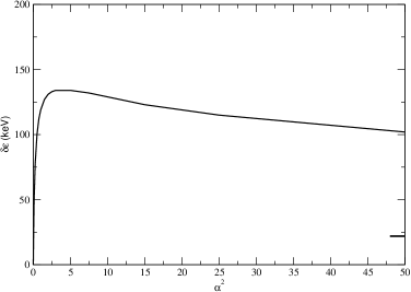
Figure 1: Effect of the correlation function from Eq. (56) on the total ground-state splitting for ${}^{16}_{\Lambda}$O as a function of $\alpha^{2}$. The value of the splitting for $\alpha^{2}=\infty$ is marked.

Nucleus	$|\delta\epsilon|$	Reference
${}^{12}_{\Lambda}$B	$\leq$ 140	[25]
${}^{16}_{\Lambda}$O	+26	[9, 10]
${}^{28}_{\Lambda}$Si	$\leq$ 400	[15]
${}^{32}_{\Lambda}$S	$\leq$ 1000	[14]
${}^{40}_{\Lambda}$Ca	$\leq$ 2200	[13]
${}^{208}_{\Lambda}$Pb	$\leq$ 2000	[15]

Table 2: Experimental constraints on the splittings in keV.

The contributions from the surviving portions of the effective interaction, the total splitting, and the resulting level orderings for a number of ground-state particle-hole splittings (as well as some excited states) are shown in Table (1). Note that the contribution labeled $V(2)$ was the portion of the interaction that was investigated in [6]; the interaction to this order failed to reproduce either the correct level ordering or splitting for the ground-state of ${}_{\Lambda}^{16}$O. Therefore, the interaction was expanded to include the higher-order gradient couplings described above. This expanded interaction, as given by Eq. (20), now gives both the proper level ordering and splitting for the ground-state of ${}_{\Lambda}^{16}$O, as shown in Table (1). Note that the inclusion of the tensor force was crucial to achieve the cancellation necessary to describe the small experimental splitting in the ground-state of ${}_{\Lambda}^{16}$O [9, 10], in agreement with previous work [8]. Similar cancellation occurs for states with $j_{1}+j_{2}+\pi=even$ (where $\pi$ denotes the parity of the system). Unfortunately, the splittings shown in Table (1) with $j_{1}+j_{2}+\pi=odd$, the ground-state of ${}_{\Lambda}^{32}$S for instance, are quite large, well outside the known experimental error bars; the experimental constraints are listed in Table (2).

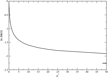
Figure 2: Effect of the correlation function from Eq. (56) on the total ground-state splitting for ${}^{32}_{\Lambda}$S as a function of $\alpha^{2}$. The value of the splitting for $\alpha^{2}=\infty$ is marked.

The fact that the interactions take the form of Yukawa potentials here implies that there is some large contribution from short-distance physics that is influencing the calculation. To correct for this problem, a correlation function was introduced to remove the short-distance physics from the integrals. The following correlation function was used here

$$V_{corr}=\left(1-e^{-\alpha^{2}m_{V}^{2}(r_{>}-r_{<})^{2}}\right)$$ (56)

A range of $\alpha^{2}$ was investigated for both ${}_{\Lambda}^{16}$O and ${}_{\Lambda}^{32}$S, the effects of which are shown in Figs. (1) and (2) respectively. Note that, regardless of $\alpha^{2}$, the correlation function does not alter the level ordering of the doublet; it changes only the magnitude of the splitting. Also, the cancellation that yields a small splitting in the ground-state of ${}_{\Lambda}^{16}$O is unaffected by the correlation function. Thus, we can improve the splittings which were quite large while retaining the small splittings that resulted from cancellation.

Technically, the proper calculation in an effective field theory such as this one is to choose an appropriate cutoff, then add a contact term for each portion of the interaction, which are essentially just constants and can be fit to experiment. However, in this case not enough data is available for nuclei in the range of $A$ accessible to this type of theory. The only relevant splitting that has been measured is the ground-state of ${}_{\Lambda}^{16}$O [9, 10]. Therefore, we conclude that at best one could claim to have a single contact term for all parts of the interaction. This is equivalent to a one parameter phenomenological calculation containing a correlation function in coordinate space meant to simulate the proper calculation.

Nucleus	$V(2)$	$NT(1)$	$\Lambda T(1)$	$TT(1)$	$TT(2)$	$\delta\epsilon$
${}^{12}_{\Lambda}$B	-26	-3	-7	-68	-17	-122
${}^{16}_{\Lambda}$N	-29	11	-37	31	50	26
	-20	-2	-6	-58	-14	-100
${}^{16}_{\Lambda}$O	-29	11	-38	31	51	26
${}^{28}_{\Lambda}$Si	-20	-1	-2	-35	-11	-68
${}^{32}_{\Lambda}$S	-15	-7	-21	-68	-13	-124
${}^{40}_{\Lambda}$Ca	-19	1	-6	19	17	13
	-22	1	4	-24	-5	-47
${}^{48}_{\Lambda}$K	-20	1	-6	19	17	12
${}^{48}_{\Lambda}$Ca	-10	0	0	-16	-11	-38
${}^{88}_{\Lambda}$Rb	-12	0	-2	14	9	10
${}^{88}_{\Lambda}$Sr	-6	0	0	-8	-5	-19
${}^{208}_{\Lambda}$Pb	-1	0	0	-3	-2	-7

Table 3: Calculation of the s_1/2-doublets (and some excited state splittings for ${}^{16}_{\Lambda}$N and ${}^{40}_{\Lambda}$Ca) in select single $\Lambda$-hypernuclei (in keV) using the correlation function from Eq. (56). Here the value of $\alpha^{2}=0.044$ was used.

The value of the cutoff that reproduced a splitting of +26 keV in the ground-state of ${}_{\Lambda}^{16}$O is $\alpha^{2}=0.044$; this translates into a momentum space cutoff of $\Lambda=\alpha^{2}m_{V}^{2}\sim 160$ MeV. The results of calculations conducted with this cutoff are shown in Table (3). All of the splittings are now within the experimental error bars.

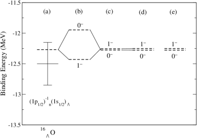
Figure 3: The ground-state of ${}^{16}_{\Lambda}$O is plotted here. (a) is the experimental level and error bars [13] along with the single-particle energy level [6], (b) is the splitting determined from $V(2)$, (c) is the splitting determined from the expanded interaction in Eq. (55), (d) is the expanded interaction with the cutoff of $\alpha^{2}=0.044$, and (e) is the experimental splitting [9, 10].

Fig. (3) shows the experimental error bars from the $\left(\pi^{+},K^{+}\right)$ reaction [13], the single-particle energy level determined from the self-consistent equations, the splitting and level ordering corresponding to the $V(2)$ contribution [6], the splitting and level ordering determined from the expanded interaction given by Eq. (55) without the correlation function and with the correlation function where $\alpha^{2}=0.044$, and the experimental doublet and level ordering [9, 10] for ${}_{\Lambda}^{16}$O. Figs. (4) – (7) show, for a range of nuclei taken from Table (1), the same contributions as Fig. (3) except that the experimental splittings have not been measured for these states. One can see from Figs. (3) and (6) that the addition of the tensor force caused the level ordering to flip and decreased the size of the splitting. In addition, the correlation function has only a limited effect on the size of the splitting. In contrast, one can see from Figs. (4), (5), and (7) that the tensor force is an additive contribution to the spin-spin force, hence the splitting becomes large. Also, the effect of the correlation function with this particular $\alpha$ is to decrease the splitting size to within the known experimental constraints. Again, note that the level orderings for the expanded interaction are unaffected by the correlation function for all cases.

The predicted ground-state of ${}_{\Lambda}^{12}$B is $2^{-}$, as seen in Fig. (5). This is inconsistent with an analysis of the emulsion data in [26] that determined the ground-state spin of this nucleus to be 1. However, this theory relies on spherical symmetry and there is evidence that ${}_{\Lambda}^{12}$B is heavily deformed. Also, it should be mentioned that this nucleus may in fact be too small for this type of mean-field approach. A resolution to this discrepancy will be the subject of future work.

In conclusion, we have developed a method to calculate the doublet splittings of select ground-state single $\Lambda$-hypernuclei. This method consists of supplementing the self-consistent single-particle equations by constructing an effective interaction to simulate the residual particle-hole interaction. The form of the effective interaction used here follows directly from the underlying lagrangian. Note that this formulation of the problem contains no free parameters. Retaining only the leading-order interaction terms, this calculation was conducted in [6]; this level of truncation in the residual interaction was inadequate to describe either the doublet size or level ordering in the ground-state of ${}_{\Lambda}^{16}$O. To improve on this calculation, we included in this effective interaction the contributions that contained gradient couplings to the neutral vector field; this incorporated a tensor force into the calculation known to play a crucial role in these systems that did not appear at leading-order. Cancellation occurs for the states that satisfy $j_{1}+j_{2}+\pi=even$, flipping the sign from the simple leading-order spin-spin interaction. However, the contributions are additive for the states satisfying $j_{1}+j_{2}+\pi=odd$, resulting in splittings that lie outside the known experimental error bars. It turns out that the integrals are dominated by short-distance physics; as a result, a cutoff was introduced to reduce this contribution. This cutoff did not effect the level orderings of any state; it did however, reduce the size of the splittings for states with $j_{1}+j_{2}+\pi=odd$ to within the experimental constraints while simultaneously retaining the cancellation the yielded small splittings in the states $j_{1}+j_{2}+\pi=even$. Thus, we obtain a realistic description of the effect of the tensor couplings on the doublet orderings and splittings.

I would like to thank Dr. B. D. Serot and Dr. J. D. Walecka for their support and advice, their careful reading of the manuscript, and their helpful comments. This work is supported by Indiana University and the State of Indiana at the Indiana University Nuclear Theory Center, 2401 Milo Sampson Lane, Bloomington, IN, 47408.

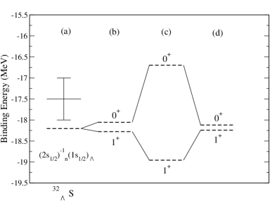
Figure 4: The ground-state of ${}^{32}_{\Lambda}$S is plotted here. (a) is the experimental level and error bars [14] along with the single-particle energy level [6], (b) is the splitting determined from $V(2)$, (c) is the splitting determined from the expanded interaction in Eq. (55), and (d) is the expanded interaction with the cutoff of $\alpha^{2}=0.044$.

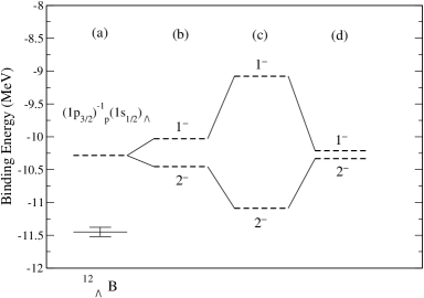
Figure 5: The ground-state of ${}^{12}_{\Lambda}$B is plotted here. (a) is the experimental level and error bars [25] along with the single-particle energy level [6], (b) is the splitting determined from $V(2)$, (c) is the splitting determined from the expanded interaction in Eq. (55), and (d) is the expanded interaction with the cutoff of $\alpha^{2}=0.044$.

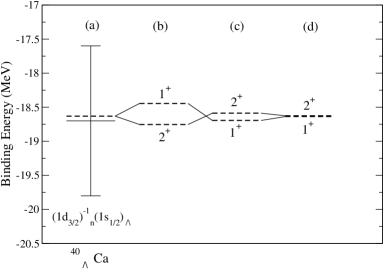
Figure 6: The ground-state of ${}^{40}_{\Lambda}$Ca is plotted here. (a) is the experimental level and error bars [13] along with the single-particle energy level [6], (b) is the splitting determined from $V(2)$, (c) is the splitting determined from the expanded interaction in Eq. (55), and (d) is the expanded interaction with the cutoff of $\alpha^{2}=0.044$.

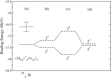
Figure 7: The ground-state of ${}^{28}_{\Lambda}$Si is plotted here. (a) is the experimental level and error bars [15] along with the single-particle energy level [6], (b) is the splitting determined from $V(2)$, (c) is the splitting determined from the expanded interaction in Eq. (55), and (d) is the expanded interaction with the cutoff of $\alpha^{2}=0.044$.

References

[1]
W. Kohn,
Rev. Mod. Phys. 71 (1999) 1253.
[2]
B.D. Serot and J.D. Walecka,
Inter. J. of Mod. Phys. E 6 (1997) 515.
[3]
R.J. Furnstahl, B.D. Serot, and H-B Tang,
Nucl. Phys. A 615 (1997) 441;
Nucl. Phys. A 640 (1998) 505 (E).
[4]
R.M. Dreizler and E.K.U. Gross:
Density Functional Theory,
Springer-Verlag (Belin, 1990).
[5]
R.J. Furnstahl,
Phys. Lett. B 152 (1985) 313.
[6]
J. McIntire,
Acta Phys. Pol. B 35 (2004) 2261.
[7]
D.J. Millener, A. Gal, C.B. Dover, and R.H. Dalitz,
Phys. Rev. C 31 (1985) 499.
[8]
D.J. Millener,
Nucl. Phys. A 754 (2005) 48c;
Nucl. Phys. A 691 (2001) 93c.
[9]
H. Tamura,et al.,
Nucl. Phys. A 754 (2005) 58c;
Mod. Phys. Lett. 18 (2003) 85.
[10]
M. Ukai,et al.,
Nucl. Phys. A 754 (2005) 70c.
[11]
G.M. Urciuoli,et al.,
Nucl. Phys. A 691 (2001) 43c.
[12]
T. Miyoshi,et al.,
Phys. Rev. Lett. 90 (2003) 232502.
[13]
P.H. Pile,et al.,
Phys. Rev. Lett. 66 (1991) 2585.
[14]
R. Bertini,et al.,
Phys. Lett. B 83 (1979) 306.
[15]
T. Hasagawa,et al.,
Phys. Rev. C 53 (1996) 1210.
[16]
V.N. Fetisov,
Nucl. Phys. A 691 (2001) 101c.
[17]
H. Muller and J. Piekarewicz,
J. of Phys. G 27 (2001) 41.
[18]
Y. Tzeng, S.Y.T. Tzeng, T.T.S. Kuo, and T-S.H. Lee,
Phys. Rev. C 60 (1999) 044305.
[19]
R. Machleidt,
in Relativistic Dynamics and Quark-Nuclear Physics,
Wiley-Interscience (New York, 1986) p71.
[20]
J.D. Walecka:
Theoretical Nuclear and Subnuclear Physics,
2nd edition, World Scientific (London, 2004).
[21]
A.R. Edmonds:
Angular Momentum in Quantum Mechanics,
Princeton University Press (Princeton, 1957).
[22]
A.L. Fetter and J.D. Walecka:
Quantum Theory of Many-Particle Systems,
McGraw-Hill (New York, 1971).
[23]
H. Matsunobu and H. Takebe,
Prog. of Theor. Phys. 14 (1955) 589.
[24]
M. Rotenberg, R. Bivins, N. Metropolis, and J.K. Wooten:
The 3-j and 6-j Symbols,
The Technology Press (Cambridge, 1959).
[25]
M. Juric,et al.,
Nucl. Phys. B 52 (1973) 1.
[26]
D. Keilczewska,et al.,
Nucl. Phys. A 238 (1975) 437.