Polishing the Lens: I Pionic Final State Interactions and HBT Correlations– Distorted Wave Emission Function (DWEF) Formalism and Examples

Abstract

The emission of pions produced within a dense, strongly-interacting system of matter in the presence of strong radial flow and absorption is described using a relativistic optical model formalism, replacing the attenuated or unattenuated plane waves of earlier emission function approaches with “distorted wave” solutions to a relativistic wave equation including a complex optical potential. The resulting distorted-wave emission function model (DWEF) is used in numerical calculations to fit HBT correlations and the resonance-corrected pion spectrum from central-collision STAR Au+Au pion data at $\sqrt{s}=200$ GeV. The parameters of the emission function are constrained by adopting a pion formation temperature taken from lattice gauge calculations and a chemical potential equal to the pion mass suggested by chiral symmetry restoration. Excellent agreement with the STAR data are obtained. The applications are extended by applying linear participant scaling to the space-time parameters of the model while keeping all other parameters fixed. This allows us to predict HBT radii over a range of centralities for both Au+Au and Cu+Cu collisions. Good agreement is found with STAR HBT data for all but the most peripheral collisions. The squares of pionic distorted wave functions, obtained as exact numerical solutions to the wave equation, are displayed and significant differences with the results of using the familiar eikonal approximation are found. Using the eikonal approximation leads to a qualitative accounting for the effects of the imaginary part of the optical potential, but fails entirely to include the effects of the real part of the optical potential. A simple example is used to illustrate that an attractive optical potential can have large effects on extracting radii and can also lead to oscillations in radii measured at low momenta.

I Introduction

Measurements of the two-particle momentum correlations between pairs of identical particles have been used to study the space-time structure of the “fireball” produced in the collision between two heavy ions moving relativistically. The quantum statistical effects of symmetrization cause an enhancement of the two-boson coincidence rate at small momentum differences that can be related to the space-time extent of the particle source. This method, called HBT interferometry, has been applied extensively in recent experiments at the Relativistic Heavy Ion Collider (RHIC) by the STAR and PHENIX collaborations. See the reviewsPratt:wm ; Wiedemann:1999qn ; Kolb:2003dz ; Lisa:2005dd .

The invariant ratio of the cross section for the production of two pions of momenta ${\bf p}_{1},{\bf p}_{2}$ to the product of single particle production cross sections is analyzed as the correlation function $C({\bf p}_{1},{\bf p}_{2})$. We define ${\bf q}$=${\bf p}_{1}$–${\bf p}_{2}$ and ${\bf K}$=$({\bf p}_{1}$+${\bf p}_{2})/2$, with ${\bf K}_{T}$ as the component perpendicular to the beam direction. (We focus on mid-rapidity data, where ${\bf K}={\bf K}_{T}$.) The correlation function can be parameterized for small ${\bf q}$ as $C({\bf q},{\bf K})-1\approx\lambda\exp{(-R_{O}^{2}q_{O}^{2}-R_{S}^{2}q_{S}^{2}-R_{L}^{2}q_{L}^{2})}\approx\lambda(1-R_{O}^{2}q_{O}^{2}-R_{S}^{2}q_{S}^{2}-R_{L}^{2}q_{L}^{2})\;(q_{i}R_{i}\ll 1),$ where $O,S,L$ represent directions parallel to ${\bf K}_{T}$, perpendicular to ${\bf K}_{T}$ and the beam direction, and parallel to the beam directionBP-HBT . Early Rischke:1996em and recent Kolb:2003dz hydrodynamic calculations predicted that a fireball evolving through a quark-gluon-hadronic phase transitions would emit pions over a long time period, causing a large ratio $R_{O}/R_{S}$. The puzzling experimental result that $R_{O}/R_{S}\approx 1$ Adler:2001zd is part of what has been called “the RHIC HBT puzzle” Heinz:2002un .

Another part of the puzzle is that the measured radii depend strongly on the average momentum $K$, typically decreasing in size by about 50% over the measured range. This dependence of a geometrical parameter on the probe momentum shows immediately that the radii are not simply a property of a static source. The influence of the interactions between the pionic probe and the medium, as well as the effects of transverse flow, must be taken into account when extracting the radii. The medium at RHIC seems to be a very high density, strongly interacting plasmaGyulassy:2004zy , so that any pions made in its interior would be expected to interact strongly.

We studied the effects of including the pionic interactions in previous workCramer:2004ih , finding that the only way to simultaneously describe the measured HBT radii and pionic spectra is to include the effects of pion-medium final state interactions by solving the relevant relativistic wave equation. These interactions are so strongly attractive that the pions can be taken as propagating through a system with a restored chiral symmetry.

The principal aim of the present work is to present a detailed treatment of the formalism that will allow wide application of our technique, and we present some new applications here. We also provide specific simple examples to demonstrate that the effects of pionic interactions cause the measured sizes of the medium to be different than the true sizes. Furthermore, we shall explicitly demonstrate that classical treatments of the pion-medium interactions, based on using the eikonal approximation for solutions of the wave equation are not valid.

An outline of the remainder of this paper follows. Previous standard formalisms that use plane wave pions are briefly reviewed in Sect. II. The technical method of incorporating the influence of final state interactions between the pion and the medium is described in Sect. III. Pionic emission in the absence of final state interaction is described with an emission function $S_{0}$ that is of a form motivated by hydrodynamics. The connection between the symmetries of this function (for the case of head-on collisions) and the form of the pion optical potential is described in Sect. IV. The role of the complex optical potential and the use of chiral symmetry to constrain its form at low energies is explained in Sect. V. The the specific numerical algorithm necessary to incorporate the optical potential is presented in Sect. VI. Once our approach is defined, there is only one approximation we need to make. The validity of this requires only that the source size be much larger than the inverse of the temperature. This large source approximation, LSA, is explained in Sect. VII. The resulting distorted wave emission function, DWEF, is evaluated using two different equivalent methods in Sec. VIII. In Sect. IX we apply these methods to STAR central Au+Au data at $\sqrt{s}=200$ GeV. Instead of treating the temperature of the system as a free parameter, as was done in Cramer:2004ih , we fix its value at the transition temperature $T_{c}=$ 193 MeV, obtained in the most recent lattice QCD calculationKatz:2005br .

For conventional calculations of the spectra, chemical equilibrium analyzes yield lower temperatures $T_{ch}=174$ MeV Braun-Munzinger:2001ip . A large difference between $T_{c}$ and $T_{ch}$ implies that the hadrons interact after the deconfinement transition occurs. This notion is entirely consistent with our treatment of pionic distortions which has as its fundamental assumption that pions interact in a hot dense medium before escaping to freedom. We also fix the pion chemical potential at the pion mass ($\mu_{\pi}=$ 139.57 MeV). The resulting procedure reduces the number of free parameters by two to a total of nine. Then we are able to reproduce a total of 32 data points with high accuracy. Section IX also extends earlier numerical resultsCramer:2004ih by computing the dependence of the HBT radii on the centrality in Au+Au collisions and by making predictions for Cu+Cu collisions vs. centrality. The eikonal approximation to solving the wave equation is discussed in Sect. X in which the important influence of the opacity and the vanishing of the effects of the real potential are also described. The importance of the real part of the optical potential in obtaining oscillating radii at low energies is illustrated through two examples in Sect. XI. A brief summary is presented in Sect. XII. Finally, a short appendix verifies an approximation to an integral.

II Previous Formalism – Plane wave pions

The aim is to include the effects of final state interactions of outgoing pions. We’ll begin with a brief review of the formalism previously used to describe HBT correlations for situations in which the pions do not interact with the medium.

The relevant observables are the covariant single- and two-particle emission functions defined as appropriately normalized ratios of cross sectionsGKW79

$${\cal P}_{1}({\bf p})=E{1\over\sigma_{\pi}}{d\sigma_{\pi}\over d^{3}{\bf p}}$$ (1)

$${\cal P}_{2}({\bf p}_{1},{\bf p}_{2})=E_{1}E_{2}{1\over\sigma_{\pi}}{d\sigma_{\pi\pi}\over d^{3}{\bf p}_{1}\;d^{3}{\bf p}_{2}}$$ (2)

$$\int{d^{3}p\over E}{\cal P}_{1}({\bf p})=\langle N\rangle$$ (3)

$$\int{d^{3}p_{1}\over E_{1}}{d^{3}p_{2}\over E_{2}}{\cal P}_{2}({\bf p}_{1},{\bf p}_{2})=\langle N(N-1)\rangle$$ (4)

$$C({\bf p}_{1},{\bf p}_{2})=\frac{\langle N\rangle^{2}}{\langle N(N-1)\rangle}\frac{{\cal P}_{2}({\bf p}_{1},{\bf p}_{2})}{{\cal P}_{1}({\bf p}_{1}){\cal P}_{1}({\bf p}_{2})}\to\frac{{\cal P}_{2}({\bf p}_{1},{\bf p}_{2})}{{\cal P}_{1}({\bf p}_{1}){\cal P}_{1}({\bf p}_{2})}.$$ (5)

The last step of Eq. (5) is obtained because $\langle N^{2}\rangle\gg\langle N\rangle$ for the very high energy collisions of interest here.

These observables can be expressed in terms of an emission function $S(x,K)$ that is the Wigner transform of the density matrix associated with the currents that emit the pions. The literature Wiedemann:1999qn ; GKW79 presents the single-particle emission function as

$$S_{0}(x,p)=\int{d^{4}y\over 2(2\pi)^{3}}\exp{(-ip\cdot y)}\langle{J}^{*}(x+y/2){J}(x-y/2)\rangle$$

$$=\int{d^{4}y\over 2(2\pi)^{3}}\langle e^{-ip\cdot(x+y/2)}{J}^{*}(x+y/2)e^{ip\cdot(x-y/2)}{J}(x-y/2)\rangle,$$ (6)

where $p$ is the four-momentum of an on-shell emitted pion and $J(x)$ is the current that acts as a source of pion fields. We shall assume that $J(x)$ is not altered by the presence of the produced pions. The brackets indicate that one takes an ensemble average over chaotic sources. Thus we assume that the emission process is initially uncorrelated: the pions are emitted from chaotic sources that have random phasesed73 ; GKW79 ; Kapusta:2005pt . This assumption seems consistent with analysis of data produced at SPS and RHICLisa:2005dd The second term of Eq. (6) is written to show that the emission function is determined by the product of a plane wave factor and the current that emits the pions. This is the standard result of scattering theory, if final state interactions are ignored. Here and throughout the paper we use natural units in which $\hbar$ and $c$ are unity. Our use of the subscript 0 denotes that the effects of final state interactions are ignored.

Next we discuss the relationship between the function $S_{0}(x,p)$ and the single-pion production cross section. If the source current couples linearly with the pion field (with a chosen interaction Lagrangian, $L_{I}$), and no final state interactions occur, the matrix element of the interaction $-L_{I}$ between the vacuum and single-pion final state is

$$\widetilde{J}(p)\equiv\int d^{4}xe^{ip\cdot x}J(x)\;=\;\int d^{4}x\phi_{\bf p}(x)J(x),$$ (7)

where $\phi_{\bf p}=e^{ip\cdot x}$ is the solution of

$$\left({\partial^{2}\over\partial t^{2}}-\nabla^{2}+m_{\pi}^{2}\right)\phi_{\bf p}=0.$$ (8)

In this plane wave (pw) approximation, the covariant single-particle emission function can be expressed as

$${\cal P}_{1}^{\rm pw}(p)=\langle\big{|}\widetilde{J}(p)\big{|}^{2}\rangle=\int d^{4}xS_{0}(x,p),$$ (9)

The literature Wiedemann:1999qn presents the two-particle emission function as

$$S_{0}(x,K)=\int{d^{4}y\over 2(2\pi)^{3}}\exp{(-iK\cdot y)}\langle{J}^{*}(x+y/2){J}(x-y/2)\rangle.$$ (10)

The quantity that enters in the HBT correlation is $S_{0}(x,K,q)$ with

$$S_{0}(x,K,q)\equiv S_{0}(x,K)e^{-iq\cdot x}=\int{d^{4}y\over 2(2\pi)^{3}}\langle e^{-ip_{1}\cdot(x+y/2)}{J}^{*}(x+y/2)e^{ip_{2}\cdot(x-y/2)}{J}(x-y/2)\rangle\equiv S_{0}(x,p_{1},p_{2}),$$ (11)

where $p_{1},p_{2}$ are the four-momenta of the two on-shell emitted pions, and

$$q=p_{1}-p_{2},\;K={1\over 2}(p_{1}+p_{2}).$$ (12)

The brackets again indicate that one takes an ensemble average over chaotic sources. The second form, Eq. (11) shows again that products of plane-wave functions and currents determine the observables. The notation $S_{0}(x,p_{1},p_{2})$ is introduced to emphasize the two-particle nature of the emission function.

In plane wave approximation the correlation function is given by the expression

$${\cal P}_{1}^{\rm pw}(p_{1}){\cal P}_{1}^{\rm pw}(p_{2})C_{0}(p_{1},p_{2})=\langle\left|\int{d^{4}x_{1}\over 2(2\pi)^{3}}\int{d^{4}x_{2}\over 2(2\pi)^{3}}{1\over\sqrt{2}}\left(e^{ip_{1}\cdot x_{1}}e^{ip_{2}\cdot x_{2}}+e^{ip_{2}\cdot x_{1}}e^{ip_{1}\cdot x_{2}}\right)J(x_{1})J(x_{2})\right|^{2}\rangle,$$ (13)

in which the effects of the Bose statistics is explicit. One proceeds by taking the absolute square to find that the expression contains four terms. The direct terms involve $\left(e^{ip_{1}\cdot x_{1}}e^{-ip_{1}\cdot x_{1}^{\prime}}\langle J(x_{1})J^{*}(x_{1}^{\prime})\rangle e^{ip_{2}\cdot x_{2}}e^{-ip_{2}\cdot x_{2}^{\prime}}\langle J(x_{2})J^{*}(x_{2})\rangle\;{\rm plus}\;1\leftrightarrow 2\right)$ and the exchange terms involve $\left(e^{ip_{1}\cdot x_{1}}e^{-ip_{2}\cdot x_{1}^{\prime}}\langle J(x_{1})J^{*}(x_{1}^{\prime}))\rangle e^{ip_{2}\cdot x_{2}}e^{-ip_{1}\cdot x_{2}^{\prime}}\langle J(x_{2})J^{*}(x_{2}))\rangle\;{\rm plus}\;1\leftrightarrow 2\right).$ The placement of the brackets arises from the use of chaotic sources: the effects of pions produced by two different chaotic sources average to 0ed73 ; GKW79 . Using the absolute square and the previous definitions in Eq. (13) yields the result

$$C_{0}(p_{1},p_{2})=1+\frac{\left|\int d^{4}xS_{0}(x,p_{2},p_{1})\right|^{2}}{\langle\big{|}\widetilde{J}(p_{1})\big{|}^{2}\rangle\langle\big{|}\widetilde{J}(p_{2})\big{|}^{2}\rangle}.$$ (14)

III Introducing Final state interactions

Our emission function, $S_{0}$, is not meant to be the same as that obtained in conventional hydrodynamic calculations of hadronic spectral functions. In such calculationsWiedemann:1999qn the quantity $S_{0}(x,K)$ is assumed to be a local equilibrium Bose-Einstein distribution localized on a 3-dimensional freeze-out hypersurface that separates the thermalized interior of the hot dense medium from the free-streaming particles on its exteriorCooper:1974mv . Here we assume that the emitted pions (and other hadrons) undergo significant interactions while escaping the hot dense medium. The emitted pions interact both with the hot dense matter and other hadrons as they escape the system. This is emission from a coexistence phase. The purpose of the present section is to provide a formalism that allows such effects to take place, while also including the usual effects of emission from a freeze out surface.

III.1 Distorted Waves

We wish to include the effect that an escaping pion has to ”fight” its way through the medium. Our formalism relies heavily on earlier derivations in Ref. GKW79 . The effects of the fighting distort the wave away from its plane wave form dictated by Eq. (8). These interactions of the pions with the medium, represented by the optical potential $U$, lead to a modified equation (approximated as a one-body equation)

$$\left({\partial^{2}\over\partial t^{2}}-\nabla^{2}+U+m_{\pi}^{2}\right)\psi=0.$$ (15)

This equation provides an approximate treatment of the complicated final state interactions. In principle, the optical potential should be related to the underlying pion source currents. We adopt a phenomenological approach. The resulting S-matrix depends on the exact solution, $\psi_{\bf p}^{(-)}(x)$, to this equation with the out boundary condition of approaching at $t\to\infty$, the free wave $\phi_{\bf p}(x)$BJD .

Ref. GKW79 uses standard S-matrix reduction techniques to show that matrix element of the pion field between the vacuum and a one-pion final state $p$ is simply the complex conjugate of $\psi_{\bf p}^{(-)}(x)$, if the optical potential is introduced as in Eq. (15). This means that in calculating the matrix elements of $-L_{I}$ between the vacuum and multi-pion final states one simply replaces the plane wave solutions of Eq. (8) by the out-going wave solutions of Eq. (15). Thus the simple replacement:

$$e^{ip\cdot x}\to\psi_{\bf p}^{(-)*}(x)$$ (16)

is sufficient to include final state interaction effects within the optical model approximation. Therefore the single-particle emission function is given by

$$S(x,p_{1})=\int{d^{4}y\over 2(2\pi)^{3}}\langle{J}^{*}(x+y/2){J}(x-y/2)\rangle\psi_{{\bf p}_{1}}^{(-)}(x+y/2)\psi_{{\bf p}_{1}}^{(-)*}(x-y/2).$$ (17)

This expression reduces to the plane wave form $S_{0}(x,p_{1})$ Eq. (10) if the distorted wave $\psi_{{\bf p}_{1}}$ are replaced by plane waves. The two-particle emission function that includes the effects of final state interactions is obtained by replacing Eq. (10) by the result

$$S(x,p_{2},p_{1})=S(x,K,q)=\int{d^{4}y\over 2(2\pi)^{3}}\langle{J}^{*}(x+y/2){J}(x-y/2)\rangle\psi_{{\bf p}_{1}}^{(-)}(x+y/2)\psi_{{\bf p}_{2}}^{(-)*}(x-y/2),$$ (18)

which applies for calculating the two-particle emission function. In the plane wave limit, $S(x,K,q)\to S_{0}(x,K)e^{-iq\cdot x}.$

Physical observables for the emission of two pions of momenta $p_{1},p_{2}$ are determined by the correlation function $C(q,K)\quad(K={1\over 2}(p_{1}+p_{2}),\;q=p_{1}-p_{2})$, which is given by

$$C(q,K)=1+\frac{|\int d^{4}xS(x,K,q)|^{2}}{\int d^{4}xS(x,p_{1})\int d^{4}xS(x,p_{2})}.$$ (19)

One obtains the usual expression (14) if the wave functions $\psi_{\bf p}^{(-)}$ are replaced by plane wave functions ($\psi_{\bf p}^{(-)}(x)\to e^{-ip\cdot x}$).

The expression (18) contains the ensemble average of the currents. This may be expressed in terms of $S_{0}(x,K)$ by taking the Fourier transform of Eq. (6). We then obtain the convolution formula:

$$S(x,K,q)=\int d^{4}K^{\prime}S_{0}(x,K^{\prime})\int{d^{4}y\over(2\pi)^{4}}\;e^{iK^{\prime}\cdot y}\psi_{{\bf p}_{1}}^{(-)}(x+y/2)\psi_{{\bf p}_{2}}^{(-)*}(x-y/2),$$ (20)

where the subscripts indicate the momenta $p_{1},p_{2}$ of the detected pions and $K={1\over 2}(p_{1}+p_{2})$. The quantity $S(x,K,q)$ is used to compute experimental observables in the same way that $S_{0}$ was previously used. This is the distorted wave emission function DWEF formalism. The expression (20) is the coordinate space version of Eq. (5.25) of Ref. GKW79 .

We emphasize that $S_{0}$ (which reflects the true properties of the source) is no longer directly related to observables–the appearance of distorted waves obscures the relationship between the data and the true properties of the source.

III.2 Extracting HBT radii

The correlation function of Eq. (19) are related to HBT radii in two different ways. In the first method, one treats the momentum differences $q_{O,S,L}$ as small quantities and then expands keeping terms to second order so that:

$$C(q,K)-1\approx 1-q_{O}^{2}R_{O}^{2}-q_{S}^{2}R_{S}^{2}-q_{L}^{2}R_{L}^{2},$$ (21)

where $q_{O}$ is the transverse component that is parallel to the direction of ${\bf K}$, $q_{S}$ is the transverse component that is perpendicular to the direction of ${\bf K}$, and $q_{L}$ is the longitudinal component. Here and below, because we are focusing on central collisions we ignore the $q_{O}q_{L}R_{OL}^{2}$ cross term. Another parameterization is

$$C(q,K)-1\approx\exp(-q_{O}^{2}R_{O}^{2}-q_{S}^{2}R_{S}^{2}-q_{L}^{2}R_{L}^{2}),$$ (22)

In practice, describing data and extracting radii require using:

$$C(q,K)-1\approx\lambda\exp(-q_{O}^{2}R_{O}^{2}-q_{S}^{2}R_{S}^{2}-q_{L}^{2}R_{L}^{2}),$$ (23)

$$C(q,K)-1\approx\lambda(1-q_{O}^{2}R_{O}^{2}-q_{S}^{2}R_{S}^{2}-q_{L}^{2}R_{L}^{2}).$$ (24)

Here the reduction factor $\lambda$ (typically about 1/2) is the fraction of pairs that originate in the space-time region relevant for correlations, see the review Lisa:2005dd . Current understanding Lisa:2005dd is that the HBT data are consistent with incoherent emission, and accounting for the many pions that are produced by the decays of resonances far outside the collision region can reproduce the factor $\lambda.$ These “halo” pions do not have a BE-enhanced correlation in the $q$ region measured with the pions emitted from the core of hot dense matter, but they cannot be experimentally separated from the latter.

Our calculations employ the core-halo model core-halo in which pions are assumed to arise either from the hot, dense core or from the halo. This model is a simplified version of more detailed treatments of resonance decays that are discussed in the review Wiedemann:1999qn .

The influence of resonances affects the extraction of radii and the measurements of the pion spectrum in different ways. We account for this in our phenomenological analysis, see the erratum of Ref. Cramer:2004ih and Sect. IX-A. Here we note only that effects of pions produced by short-lived resonances (such as $\Delta,\rho,\cdots$) that are not explicitly included in the pionic wave equation are included in the function $S_{0}$. The pions resulting from long lived resonances are not included in $S_{0}$. Pions resulting from the decay of slowly moving $\Omega$ mesons that occur inside the dense matter system are included in $S_{0}$, but the pions from rapidly moving $\omega$ mesons that decay outside of the system are not included in $S_{0}$.

The approximate forms (23,24) provide two ways to extract radii. The former suggests that

$$R_{i}^{2}={1\over q_{i}^{2}}\ln{\lambda\over C(q_{i},K)-1},\quad i=O,S,L$$ (25)

while the latter implies

$$R_{i}^{2}={1\over q_{i}^{2}}{C(q_{i},K)-1\over\lambda},\quad i=O,S,L$$ (26)

Eq. (25) can be used for values of $q_{I}$ such that $(C-1)/\lambda$ can be approximated by a Gaussian function. The use of Eq. (24) requires that $q_{i}R_{i}\ll 1$. We show below in Sect. VIII that, while the correlation functions are not Gaussians (so that the squared radii are not moments of the correlation function), the Gaussian parameterization is quite accurate at the modest (but not very small) values of $q_{i}\sim 30$ MeV/c that dominate the experimental extraction of radii.

IV Symmetries of $S_{0}(x,K)$ and the form of the pion distorted waves

We use the hydrodynamic parameterization of the source of Ref. CL96a ; H96 ; Tomasik:1997eq . Generally based on the Bjorken tube model, it is given by

$$S_{0}(x,K)\,d^{4}x = {M_{\perp}\cosh(\eta-Y)\over(2\pi)^{3}}\;{1\over\exp\left[{(K\cdot u(x)-\mu_{\pi})\over T(x)}\right]-1}\;\rho(b)\exp\left[-{{(\eta-\eta_{0})}^{2}\over 2(\Delta\eta)^{2}}\right]$$ (27)

$$\times{\tau\,d\tau}\left[\frac{1}{\sqrt{2\pi(\Delta\tau)^{2}}}\;\exp\left(-{(\tau-\tau_{0})^{2}\over 2(\Delta\tau)^{2}}\right)\right]\,d\eta\,b\,db\,d\phi,$$

$$d^{4}x = \tau d\tau\;d\eta\;b\;db\;d\phi.$$ (28)

Here, $\mu_{\pi}$ is the pion chemical potential, the variables $(b,\phi)={\bf b}$ are equivalent to ${\bf x}_{\perp}$,$\;\eta={1\over 2}\ln{t+z\over t-z},\;\tau=\sqrt{t^{2}-z^{2}},M_{T}=\sqrt{K_{\perp}^{2}+m_{\pi}^{2}},Y={1\over 2}\ln{E_{K}+K_{z}\over E_{K}-K_{z}}.$ The factor in the brackets involving $\tau$ has the same normalization as the delta function: $\delta(\tau-\tau_{0})$. We use a Bose-Einstein distribution instead of the Boltzmann distribution of Ref. Tomasik:1997eq and also allow the transverse density $\rho(b)$ to have a general form instead of a Gaussian. Note that the model contains the parameters: $R,\eta_{0},\Delta\eta,\Delta\tau,\tau_{0},\eta_{f}$. As stated originally, temperature gradients were included, but we treat the temperature as a constant for our numerical calculations. We shall see below that our formalism can easily be generalized to allow the temperature to vary as a function of $b$.

The longitudinal $\eta,\tau$ and transverse $({\bf b},{\bf K})$ variables can be separated in the following form:

$$S_{0}(x,K) = {\cal S}_{0}(\eta,\tau,Y)\;B_{\eta}({\bf b},{\bf K})$$ (29)

$$B_{\eta}({\bf b},{\bf K}) \equiv {M_{\perp}\over\exp[(K\cdot u-\mu_{\pi})/T]-1}\rho(b)$$ (30)

$${\cal S}_{0}(\eta,\tau,Y) \equiv {\cosh(\eta-Y)\over(2\pi)^{3}}\;\exp\left[-{{\eta}^{2}\over 2(\Delta\eta)^{2}}\right]\frac{1}{\sqrt{2\pi(\Delta\tau)^{2}}}\;\exp\left[-{(\tau-\tau_{0})^{2}\over 2(\Delta\tau)^{2}}\right].$$ (31)

Here $\rho(b)$ is a function, normalized as $\rho(0)=1$ that represents the transverse density. To be specific we use

$$\rho(b)=[1/(\exp((b-R_{WS})/a_{WS})+1)]^{2}.$$ (32)

This distribution has a correct exponential fall-off at large values of $b$, and different choices of the parameters $R_{WS},\;a_{WS}$ allow a variety of shapes to be assumed.

We concentrate on the kinematics of the STAR experiment which detects pions within half a unit of rapidity of moving perpendicular to the beam, so we take $Y=0$. This means that the average momentum is transverse: ${\bf K}={\bf K}_{\perp}={\bf K}_{T}$. With colliding beams of equal mass and energy there is a fore-aft symmetry along the longitudinal axis, so that we use $\eta_{0}=0.$ Therefore it is useful to define

$${\cal S}_{0}(\eta,\tau)\equiv{\cal S}_{0}(\eta,\tau,Y=0).$$ (33)

The velocity field $u(x)$ describing the dynamics of the expanding source is parameterized by WSH96

$$u^{\mu}(x)=\left(\cosh\eta\cosh\eta_{t}(b),\,\cos\phi\,\sinh\eta_{t}(b),\,\sin\phi\,\sinh\eta_{t}(b),\,\sinh\eta\cosh\eta_{t}(b)\right),$$ (34)

with $\phi$ the angle between ${\bf K}_{\perp}$ and ${\bf u}$ (or when appearing in the single-particle emission function, it is the angle between ${\bf p}_{i}$ and ${\bf u}$). Eq. (34) implements a boost-invariant longitudinal flow profile $v_{L}=z/t$, with a linear radial profile of strength $\eta_{f}$ for the transverse flow rapidity:

$$\eta_{t}(b)=\eta_{f}{b\over R_{WS}}\,.$$ (35)

The exponent that enters in the Bose-Einstein distribution is given by the four-vector dot product:

$$K\cdot u(x)=M_{\perp}\cosh(\eta-Y)\cosh\eta_{t}(b)-K_{\perp}\,\sinh\eta_{t}(b)\,\cos\phi\,.$$ (36)

The presence of a non-vanishing value of $\eta_{f}$ causes the emission function to depend on both $K$ and $M_{\perp}$. The Bose-Einstein distribution of Eq. (30) is evaluated as a sum of Boltzmann distributions:

$${1\over\exp\left[{K\cdot u(x)-\mu_{\pi}\over T}\right]-1}=\sum_{n=1}^{\infty}\exp({-K\cdot u+\mu_{\pi}\over T_{n}}),\;T_{n}\equiv{T\over n}.$$ (37)

The parameterization (27) is motivated by hydrodynamical models with approximately boost-invariant longitudinal dynamics. It uses thermodynamic and hydrodynamic parameters and appropriate coordinates. The “emission function” given above was originally intended to parameterize the distribution of points of last interaction in the source. In conventional treatments, the Cooper-FryeCooper:1974mv matching procedure is used to obtain distributions of detected particles. Our approach is more general. We assume that pions can be formed at any space-time point (including but not limited to the freeze-out surface) during the collision, and propagate through the dense medium while interacting before being detected. Thus we take $S_{0}(x,K)$ to be the emission function in the absence of final state interactions.

We note that the emission function of Eq. (27) has been previously used in the “blast-wave model” Retiere:2003kf , and we would like to comment on the differences between our formalism and that model. These include:

• The blast-wave model does not attempt to reproduce the normalization of the spectrum, and sets the chemical potential $\mu_{\pi}$ to 0. We find that taking $\mu_{\pi}$ to be the pion mass allows us to reproduce both the normalization and the shape of the pion momentum spectrum.

• The blast-wave model uses the smoothness approximation and computes HBT radii as moments of the emission function.

• The blast-wave model uses plane waves and therefore omits the effects of the optical potential.

• The blast-wave model uses a parameterized emission function to describe the six-dimensional distribution of pions on some freeze-out hypersurface, while the emission function of the DWEF model describes the initial emission of pions within the hyper-volume of the hot, dense medium produced by the collision. Therefore, it is not appropriate to compare emission-function parameters like $T$ and $R$ that are derived from blast-wave fits with those of the present model.

V Final state interactions and the optical potential

The salient feature of the 200 GeV data is the high density of the produced matter, so we treat the effects of pion final state interactions with a dense medium. We adopt a single-channel approach that uses the interaction–distorted incoming wave $\Psi_{{\bf p}_{1}}^{(-)*}(x_{1})$.

We assume that the matter produced in the central region of the collision is cylindrically symmetric with a very long axis, so that an expression of the form (29) is valid. In that case, the optical potential $U$ representing the interaction between a pion and the medium is a complex, azimuthally-symmetric function depending on pion momentum and local density. Within our formalism the influence of some time-dependent effects in $U$ introduced by the time-dependent source $S_{0}$ is incorporated in the energy dependence of the optical potential, and the pion-medium interaction time is restricted by $S_{0}$.

The optical potential accounts for the interaction between each pion and the surrounding medium, but does not include the interaction between the two pions. In particular, the Coulomb interaction is known to be important. The experimental analysis removes this effect before extracting radii from the data. The Coulomb interaction between pions is of long range and its important effects occur when the pions are outside the medium. Indeed, specific analyzes show that Coulomb effect occur only at very low relative momenta STARHBT . In contrast, the optical potential acts only when pions are inside. We therefore expect that presence of the optical potential would not influence the removal of the Coulomb interaction. A quantitative treatment of the effect of the optical potential on the removal of Coulomb effects would involve solving a three-body problem. This is not warranted at the present stage of development, but might eventually become worthwhile.

The optical potential accounts for situations in which the pion changes energy or disappears entirely due to its interactions with the dense medium. We do not assume to know the content of the dense medium, and therefore will use a phenomenological optical potential. But it is worthwhile to consider a simple example to get an idea about how large the optical potential can be. Suppose, e.g., that the medium is a gas of pions. Then $\pi\pi$ scattering would be the origin of $U$. In the impulse approximation, the central optical potential would be $U_{0}=-4\pi f\rho_{0}$, where $f$ is the complex forward scattering amplitude and $\rho_{0}$ the central density. For low energy pion-pion interactions, $4\pi$Im$[f(p)]=p\sigma,$ with $\sigma\approx 1\;$mb. At a momentum $p=1~{}\rm{fm}^{-1}=197.3$ MeV/c, using a pion density about ten times the baryon density of ordinary nuclear matter, Im$[U(0)]\approx-0.15~{}\rm{fm}^{-2}$, representing significant opacity.

The optical potential must be an analytic function of energy, and therefore the existence of an imaginary part mandates the existence of a real part. Thus, any analysis needs to treat $U$ as a complex function. Under certain circumstances the real part can be very large. For example, if two interacting pions each have less energy than half of the rho meson mass, the final state interactions caused by virtual transitions to a rho meson would be strongly attractive. Additionally, the influence of chiral symmetry restoration can lead to a strong real part. This is discussed next.

V.1 Chiral Symmetry Restoration

Suppose the dense medium is one in which chiral symmetry is restored. This means that the value of the quark condensate vanishes, an effect that could be caused by an increase in temperature or density. The pion mass is proportional to the quark condensate via the GMOR relation Gell-Mann:1968rz

$$m_{\pi}^{2}f_{\pi}^{2}=-{m_{u}+m_{d}\over 2}\langle 0|\bar{u}u+\bar{d}d|0\rangle,$$ (38)

where $f_{\pi}$ is the weak pion decay constant $\approx 93$ MeV. It is believed that $m_{\pi},f_{\pi}$ and the condensate $\langle 0|\bar{u}u+\bar{d}d|0\rangle$ all depend on temperature and density. If one takes the Brown-RhoBrown:1991kk scaling relation for $f_{\pi}$ and the perturbatively calculated temperature dependence of the condensate, the pion mass is proportional to the cube root of the condensate, and therefore vanishes for sufficiently large temperatures. See the reviews Koch:1996vt . Suppose the optical potential arises only from the temperature dependence of the pion mass. Then the Klein-Gordon equation would take the form:

$$(-\nabla^{2}+m_{\pi}^{2}(T))\psi=(p^{2}+m_{\pi}^{2})\psi,$$ (39)

for regions inside the medium. The effects of the medium are incorporated through the difference between $m-\pi^{2}(T)$ and $m_{\pi}^{2}$. If one re-writes Eq. (39) as a Klein-Gordon equation $(-\nabla^{2}+U)\psi=p^{2}\psi,$ then the optical potential takes the form:

$$U(b)=(m_{\pi}^{2}(T)-m_{\pi}^{2})\rho(b),$$ (40)

in which the finite extent of the medium is accounted for by the factor $\rho(b)$. If $m_{\pi}(T)$ approaches zero, the optical potential is attractive with magnitude $m_{\pi}^{2}.$

A more recent study by Son & StephenovSon:2002ci provides a more detailed treatment of the effects of chiral restoration in which the general $p$-wave nature of the low-energy interaction between pions and any target is included. We are guided by this work. Son & Stephenov use the dispersion relation for low momentum pions in infinite nuclear matterboy ; Son:2002ci :

$$\omega^{2}=u_{\pi}^{2}(\hat{p}^{2}+m_{\pi}(T)^{2}),$$ (41)

where $\hat{p}^{2}$ is the infinite-sized matter version of $-\nabla^{2}$. The quantity $u_{\pi}$ is termed the pion velocity, even though it is only that when $m_{\pi}(T)$ vanishes. The term $m_{\pi}(T)$ is denoted the pion screening mass. This quantity appears in the expression for the static Euclidean pion correlatorSon:2002ci . The energy of a pion at ${\bf p}=0$ is termed the pion pole mass. The free pion mass is $m_{\pi}$. In Ref. Son:2002ci Eq. (41) applies only for $T<T_{c}$. For larger temperatures, chiral symmetry is restored and pions are massless.

Defining $t\equiv(T_{c}-T)/T_{c}$, SS find $m_{\pi}^{2}(T)\sim t^{\beta-\nu},\;u^{2}\sim t^{\beta}$, with $\beta<\nu$, e.g $\nu=.73,\beta=.38$Baker:1977hp . These equations are valid for temperature close to (but not too close to) the critical point. Another view about the dispersion relation can be found in Ref. sas . This general discussion about the influence of chiral restoration provides some guidance, but does not tell us exactly to use.

We wish to obtain an equivalent optical potential and see if it is attractive or repulsive. Use the Klein Gordon equation in the form

$$\hat{p}^{2}+U+m_{\pi}^{2}=p^{2}+m_{\pi}^{2}.$$ (42)

In regions outside the dense medium where $U=0$, the operator $\hat{p}^{2}$ is simply the square of the momentum, $p^{2}$. Subtract (42) from (41) to obtain

$$U=u_{\pi}^{2}m_{\pi}^{2}(T)-m_{\pi}^{2}+(u_{\pi}^{2}-1)\hat{p}^{2},$$ (43)

an expression that is the sum of two negative definite terms. This form can be simplified by using the wave equation (42) to remove term $\hat{p}^{2}$. Then one finds a momentum-dependent optical potential:

$$U={u_{\pi}^{2}m_{\pi}^{2}(T)-m_{\pi}^{2}+(u_{\pi}^{2}-1)p^{2}\over u_{\pi}^{2}}.$$ (44)

Note that if $u_{\pi}$ becomes really small the optical potential becomes very strongly attractive.

For matter of finite size, the term $\hat{p}^{2}$ can also be interpreted as $-\nabla\cdot c\nabla$ which is the Kisslinger term lsk . For infinite nuclear matter only forward scattering occurs and the two terms are identical, but differences may arise for scattering from media of finite size. One can not tell the difference between the two terms at the start, so that we find a general form

$$U(b)=-(w_{0}+w_{2}(1-\epsilon)p^{2})\rho(b)-\epsilon w_{2}\nabla\rho(b)\cdot\nabla,$$ (45)

with both the real and imaginary parts of $w_{0},w_{2},\epsilon$ positive for attractive interactions, and $\rho(b)$ taken from Eq. (32). This simple form is strictly valid only for low-energy pions. The limit of an infinite tube is used to write $U$ as independent of $z$. We find for the 200 GeV data, that for temperatures below our assumed value of 193 MeV the fitting prefers a very small value of the Kisslinger term, so we simply set $\epsilon=0$. We also take $w_{0}$ real (so that there is no opacity at p=0). We shall see below, that if the temperature is set to a value greater than 193 MeV, the fit is improved by including the gradient terms at about the 20% level ($\epsilon\approx 0.2$). The simple form Eq. (45) is sufficient to account for the data we study, $K_{T}\leq 600$ MeV/c, but we remind the reader that the interaction strength does not grow as $p^{2}$ for $p$ much greater than about 400 MeV/c.

We shall discuss the precise parameters of the optical potential in subsequent sections. For now we may simply proceed using the assumption that $U$ is a complex, azimuthally-symmetric function depending on pion momentum and local density of the form of Eq. (45).

VI Finding $\psi^{(\pm)}({\bf x})$

The evaluation of the emission function (20) requires performing an eight dimensional integral using a distorted wave. We shall use symmetries to reduce the number of numerical evaluations. Doing this depends on obtaining a compact expression for the distorted wave. In the present section, we show how the distorted waves are evaluated.

The first step is to realize that the function $\psi_{\bf p}^{(-)}(x)$ represents an energy-eigenfunctionGKW79 provided the optical potential does not change with time. We shall show below that the value of $\delta\tau$ is not large. Thus the the time-independent optical potential that we use can be thought of as a time-averaged optical potential. So we have

$$\psi_{\bf p}^{(-)}(x)=e^{-i\omega_{p}\;x^{0}}\Psi_{\bf p}^{(-)}({\bf x}).$$ (46)

To proceed we need to examine the properties of the wave function $\psi_{\bf p}^{(-)}({\bf x})$. It is conventional to compute $\psi_{\bf p}^{(+)}({\bf x})$, and we will follow this convention. Then we use time reversal invariance in the form

$$\Psi_{\bf p}^{(-)}({\bf x})={\Psi_{-{\bf p}}^{(+)}}^{*}({\bf x})$$ (47)

to obtain the desired wave function.

The next step is to realize that for central collisions, $Y=0$, the emission function (31) has a cylindrical symmetry. This means that the expected optical potential is azimuthally symmetric. If we take the matter to have the form of a very long tube, the optical potential will be independent of $z$. Then one obtains a solution that takes a product form

$$\Psi_{{\bf p}_{1,2}}^{(-)}({\bf x}) = e^{\mp iq_{L}z/2}\psi_{{\bf p}_{1,2}}^{(-)}({{\bf x_{\perp}}={\bf b}}),$$ (48)

$$\quad{\bf p}_{1,2} = {\bf K}\pm{\bf q}/2\pm{\bf\widehat{z}}\;q_{L}/2,$$ (49)

where the vector ${\bf q}$ is defined as a transverse vector ${\bf q}\cdot{\bf\widehat{z}}=0$.

We may obtain the wave function $\psi_{\bf p}^{(+)}({{\bf b}})$ by solving the wave equation

$$\left(-\nabla_{\perp}^{2}+U(b)\right)\psi_{\bf p}^{(-)*}({{\bf b}})=p^{2}\psi_{\bf p}^{(-)*}({{\bf b}}).$$ (50)

If $U=0,\;\psi_{\bf p}^{(+)}({{\bf b}})=e^{i{\bf p}\cdot{\bf b}}$. Many previous treatments of opacity can be understood as using the eikonal approximation to obtain solutions to Eq. (50).

We take the optical potential to have the azimuthally-symmetric form of Eq. (45) so that the solution for $\psi_{\bf p}^{(\pm)}({\bf b})$ can be expanded in partial wave form in plane polar coordinates ($b\equiv\sqrt{{\bf x}_{\perp}^{2}},{\phi},\cos\phi\equiv\hat{{\bf p}}\cdot\hat{{\bf b}}$):

$$\psi_{\bf p}^{(+)}({{\bf b}})=\sum_{m=-\infty,\infty}f_{m}(p,b)i^{m}\;e^{im\phi},$$ (51)

$$\psi_{\bf p}^{(+)}({{\bf b}})=f_{0}(p,b)+2\sum_{m=1,\infty}f_{m}(p,b)i^{m}\;\cos{m\phi},$$ (52)

with (52) taking into account the invariance of the differential equation for $f_{m}$ under the interchange $b\to-b$. Note that we may use Eq. (47) to find

$$\psi_{\bf p}^{(-)*}({\bf x_{\perp}})=f_{0}(p,b)+2\sum_{m=1,\infty}f_{m}(p,b){(-i)}^{m}\;\cos{m\phi}.$$ (53)

In practice a finite number of terms is needed, with $m\leq m_{max}\approx 2pR/\hbar$.

Use Eq. (52) in (50) to find

$$\left({d^{2}\over db^{2}}+{1\over b}{d\over db}+(p^{2}-{m^{2}\over b^{2}})\right)f_{m}(p,b)-U({b^{2}\over R^{2}})f_{m}(p,b)=0.$$ (54)

Note that for large enough $b$, $U$ vanishes and the $f_{m}$ are linear combinations of Bessel $J_{m}$ and Neumann $N_{m}$ functions or Hankel functions $H_{m}^{(1,2)}$.

This differential equation can be solved numerically using the Runge-Kutta technique. One determines the wave function by matching the numerical solutions to the analytic solution

$$f_{m}(p,b)=A_{m}\left(J_{m}(pb)+T_{m}H_{m}^{(1)}(pb)\right).$$ (55)

One matches the numerical function and its derivative (at large enough $b$ so that $U=0$) so as to determine the constants $A_{m},T_{m}$. The normalization of $\psi_{\bf p}^{(\pm)}$ is such that $A_{m}=1$–asymptotically the wave is a sum of an ordinary plane wave and an outgoing wave, and the functions $f_{m}(p,b)$ can be regarded as phase shifted Bessel functions. Using the partial-wave form of two-dimensional wave function (52) will simplify the evaluation of $S(x,K)$ of Eq. (20).

VII The Distorted Wave Emission Function (DWEF) and the Large Source Approximation (LSA)

Using (46) in Eq.(20) allows the integrals over $y^{0}$ and $K^{0^{\prime}}$ to be evaluated as:

$$S(x,K,q)=\int{d^{3}K^{\prime}\over(2\pi)^{3}}S_{0}(x;K^{0},{\bf K}^{\prime})e^{i(\omega_{2}-\omega_{1})x^{0}}\int d^{3}y\;e^{-i{\bf K}^{\prime}\cdot{\bf y}}\Psi_{{\bf p}_{1}}^{(-)}({\bf x}+{\bf y}/2)\Psi_{{\bf p}_{2}}^{(-)*}({\bf x}-{\bf y}/2),$$ (56)

and using (49) allows the integrals over $y^{3}$ and ${K^{3}}^{\prime}$ to be evaluated yielding a four-dimensional integral:

$$S(x,K,q) = {1\over(2\pi)^{2}}{\cal S}_{0}(\tau,\eta)e^{iq^{0}t-iq_{l}z}\int d^{2}b^{\prime}\widetilde{B}_{\eta}({\bf b},{\bf b}^{\prime})\psi_{{\bf p}_{1}}^{(-)}({\bf b}+{\bf b}^{\prime}/2)\psi_{{\bf p}_{2}}^{(-)*}({\bf b}-{\bf b}^{\prime}/2),$$ (57)

$$\widetilde{B}_{\eta}({\bf b},{\bf b}^{\prime})\equiv\int d^{2}K^{\prime}_{T}\;B_{\eta}({\bf b},{\bf K}^{\prime}_{T})\exp\left[-i{\bf K}_{T}^{\prime}\cdot{\bf b}^{\prime}\right].$$

The result (57) still requires the evaluation of an 6-dimensional integral (over $\tau,\eta,{\bf b}^{\prime},{\bf K}^{\prime}_{T}$) to obtain the correlation function. We search for simplifications. The integral (57) simplifies if we ignore the effects of transverse flow rapidity. So to gain insight, let’s set

$$\eta_{f}=0,$$ (58)

consider a fixed value of $\eta$, and take one of the terms in the series (37). Then

$$\widetilde{B}_{\eta}({\bf b},{\bf b}^{\prime})=\rho(b)\;g({\bf b}^{\prime 2})$$ (59)

$$g({\bf b}^{\prime 2})=2\int d^{2}K_{\perp}\;M_{\perp}\exp\left[{-M_{\perp}\cosh\eta\over T}\right]\;\exp\left[-i{\bf K}_{\perp}\cdot{\bf b}^{\prime}\right]$$ (60)

Fig. 1 shows $g(b)$ for the case $T/\cosh\eta=m_{\pi}$. It is clear from (60) that the quantity $T$ controls the range of allowed values of $K_{\perp}$, so that the extent of $b^{\prime}$ is of order $1/T\approx 1\;{\rm fm}$ for $T$ = 200 MeV. This is much smaller than the size of the presumed fireball that controls the extent of $b$ in (57). Thus it is natural to think of neglecting the terms involving $\pm{\bf b}^{\prime}/2$ of (57). This however, is too extreme an approximation because it would not lead to the formalism of Sect. 1 in the plane wave limit. Instead, we use the approximation

$$\psi^{(-)}({\bf b}\pm{\bf b}^{\prime}/2)\approx e^{\mp i{\bf p}_{\perp}\cdot{\bf b}^{\prime}/2}\psi^{(-)}({\bf b})$$ (61)

This is exact in the plane wave limit, but its wider validity relies on the replacement

$$\psi_{{\bf p}_{i}}^{(-)}({\bf b}+{\bf b}^{\prime}/2)\psi_{{\bf p}_{j}}^{(-)*}({\bf b}-{\bf b}^{\prime}/2)\;g({\bf b}^{\prime 2})\approx\psi_{{\bf p}_{i}}^{(-)}({\bf b})\psi_{{\bf p}_{j}}^{(-)*}({\bf b})\;g({\bf b}^{\prime 2})\exp{(i{\bf K}_{\perp}\cdot{\bf b}^{\prime})},$$ (62)

that requires that the size of the source be much larger than ${n/T}$, where $n$ is the expansion order in the Bose-Einstein distribution (37). Our sources typically have a diameter of about 25 fm, and $T\sim 1\;{\rm fm}^{-1}$, so that $n$ must be no bigger than about 25. We achieve numerical convergence with $n<10$, so that the source is truly large enough for our approximation. We denote Eq. (62) to be the “Large Source Approximation” (LSA) and use it to immediately integrate over ${\bf b}^{\prime}$ and to obtain a simpler version of (57):

Figure 1: Plot of g(b), showing cutoff around $b=1/T$, with $T=1/m_{\pi}$ and $b$ in fm.

$$S(x,K)={\cal S}_{0}(\tau,\eta,Y)e^{i(\omega_{2}-\omega_{1})\tau\cosh\eta}e^{-iq_{L}\tau\sinh\eta}{B}_{\eta}({\bf b},{\bf K})\psi_{{\bf p}_{1}}^{(-)}({\bf b})\psi_{{\bf p}_{2}}^{(-)*}({\bf b}),$$ (63)

that is obtained for any value of $\eta_{f}$. The expansion (37) gives

$$B_{\eta}({\bf b},{\bf K})=\sum_{n=1}^{\infty}\exp({-K\cdot u+\mu_{\pi}\over T_{n}})M_{T}\rho(b)$$

$$=\sum_{n=1}^{\infty}\exp({-M_{T}\cosh\eta\cosh\eta_{t}(b)+\mu_{\pi}\over T_{n}})\exp({K_{T}\sinh\eta_{t}(b)\cos\phi\over T_{n}})M_{T}\rho(b),$$ (64)

so that Eq. (63) becomes

$$S(x,K,q)={\cal S}_{0}(\tau,\eta,Y)e^{i(\omega_{2}-\omega_{1})\tau\cosh\eta-iq_{L}\tau\sinh\eta}\sum_{n=1}^{\infty}\exp(-\gamma_{n}(b)\cosh\eta)B_{n}({\bf b},{\bf K})\psi_{{\bf p}_{1}}^{(-)}({\bf b})\psi_{{\bf p}_{2}}^{(-)*}({\bf b})$$ (65)

$$B_{n}({\bf b},{\bf K})\equiv\exp(\mu_{\pi}/T_{n})\exp(K\sinh\eta_{t}(b)\cos\phi/T_{n})\;M_{T}\rho(b)$$ (66)

$$S(x,p_{i})={\cal S}_{0}(\tau,\eta,Y)\sum_{n=1}^{\infty}\exp(-\gamma_{n}(b)\cosh\eta)B_{n}({\bf b},{\bf p}_{i})\left|\psi^{(-)}_{{{\bf p}}_{i}}({\bf b})\right|^{2},$$ (67)

$$\gamma_{n}(b)\equiv{M_{T}\cosh\eta_{t}(b)\over T_{n}}.$$ (68)

The number of terms in the summation over $n$ required to achieve an accurate result depends on the values of $\mu_{\pi},{\bf K}$. If desired the quantities $T,\mu_{\pi}$ can be treated as functions of $b$ CL96a in Eq. (66), rather than as constants, as we have done here.

VIII Correlation function

The specific form of the wave function enables us to express the correlation function as $C(q_{L}{\bf\hat{z}}+{\bf q},{\bf K})$:

$$C(q_{L}{\bf\hat{z}}+{\bf q},{\bf K})=1+\frac{|\int d^{4}xS(x,K,q)|^{2}}{\int d^{4}xS(x,p_{1})\int d^{4}xS(x,p_{2})}$$ (69)

$${\bf p}_{1,2}={\bf K}\pm q_{L}/2{\bf\hat{z}\pm{\bf q}/2}.$$ (70)

The dependence on $q_{L}$ occurs only in the numerator.

The remaining task is to perform the integral over $d^{4}x$. We use two separate approaches. The first Cramer:2004ih involves expanding $S(x,K)$, Eq. (66), as double power series in $q_{L}$ and $\tau$, keeping all terms up to second order. The second involves exact numerical integration. The two methods yield nearly identical results, with the second being more accurate and taking only slightly more computer time. We present both methods here. First, we take ${\bf q}$ to be small and make expansions Sec. VIII.1. This formalism is applied to obtain numerical results for radii and spectra in Sects. IX.1,IX.5 and Sect. IX.6. The formalism to compute the correlation functions without the use of expansion is contained in Sec. VIII.2, and this formalism is applied to compute correlation functions in Sec. IX.7.

VIII.1 Evaluation of correlation function by expansion

Now we make the above mentioned expansion keeping terms to order $q_{L}^{2}$, (and anticipate the integration over $\eta,\tau$). The term linear in $q_{L}$ is an odd function of $\eta$ so that it vanishes when the integration over $\eta$ is carried out. Use $\omega_{2}-\omega_{1}=-q_{o}\beta,\beta\equiv K_{T}/M_{T}$. Thus the expansion of Eq. (66) is

$$S(x,K)={\cal S}_{0}(\tau,\eta,Y)(1-iq_{o}\beta\tau\cosh\eta-{1\over 2}q_{o}^{2}\beta^{2}\tau^{2}\cosh^{2}\eta-{1\over 2}q_{L}^{2}\tau^{2}\sinh^{2}\eta)$$

$$\times\sum_{n=1}^{\infty}\exp(-\gamma_{n}(b)\cosh\eta)B_{n}({\bf b},{\bf K}_{T})\psi^{(-)}_{{{\bf p}}_{1}}({\bf b})\psi^{(-)*}_{{{\bf p}}_{2}}({\bf b}),$$ (71)

The effects of the $Y$ dependence of ${\cal S}_{0}(\tau,\eta,Y)$ that appears for $q_{L}\neq 0$ is the same for the numerators and denominators of the correlation functions and vanish. Hence we do not keep this explicit dependence in the intermediate steps in the following calculations.

The next step in evaluating (69) is to integrate over all $\tau,\eta$ using the measure $d\eta\tau d\tau$. The first integral to appear arises from the factor of unity appearing inside the parenthesis of (71). It is

$$I_{0}\equiv{1\over\sqrt{2\pi}\Delta\tau}\int_{-\infty}^{\infty}d\eta\cosh\eta\int_{-\infty}^{\infty}\tau d\tau\exp(-{\eta^{2}\over 2(\Delta\eta)^{2}})\exp(-{(\tau-\tau_{0})^{2}\over 2(\Delta\tau)^{2}})\exp(-\gamma_{n}(b)\cosh\eta)$$

$$\approx 2\tau_{0}\exp({1\over\Delta\eta^{2}})K_{1}(\gamma_{n}+{1\over\Delta\eta^{2}})\equiv\tau_{0}f_{0}(\xi_{n})\exp({1\over\Delta\eta^{2}}),\;f_{0}(\xi_{n})=2K_{1}(\xi_{n}),\xi_{n}\equiv\gamma_{n}+{1\over\Delta\eta^{2}}.$$ (72)

The approximation involves the replacement

$$\exp(-{\eta^{2}\over 2(\Delta\eta)^{2}})\to\exp({1\over\Delta\eta^{2}})\exp(-{1\over\Delta\eta^{2}}\cosh\eta).$$ (73)

Similar replacements are made below. The dominant contributions to the integral involve small values of $\eta$, so the approximation is expected to be very good. The appendix shows that the error involved is less than about 2%.

We proceed to use the same replacement to evaluate the remaining integrals and find

$$I_{2}\equiv{1\over\sqrt{2\pi}\Delta\tau}\int_{-\infty}^{\infty}\cosh\eta d\eta\int_{-\infty}^{\infty}\tau d\tau\exp(-{\eta^{2}\over 2(\Delta\eta)^{2}})\exp(-{(\tau-\tau_{0})^{2}\over 2(\Delta\tau)^{2}})\exp(-\gamma_{n}(b)\cosh\eta)(-iq_{0}\beta)\tau\cosh\eta$$

$$\approx(-iq_{0}\beta)(\tau_{0}^{2}+(\Delta\tau)^{2})\exp({1\over\Delta\eta^{2}})f_{2}(\xi_{n}),f_{2}(\xi_{n})=K_{0}(\xi_{n})+K_{2}(\xi_{n})=2(K_{0}(\xi_{n})+{K_{1}(\xi_{n})\over\xi_{n}}),$$ (74)

$$I_{3}\equiv{1\over\sqrt{2\pi}\Delta\tau}\int_{-\infty}^{\infty}\cosh\eta d\eta\int_{-\infty}^{\infty}\tau d\tau\exp(-{\eta^{2}\over 2(\Delta\eta)^{2}})\exp(-{(\tau-\tau_{0})^{2}\over 2(\Delta\tau)^{2}})\exp(-\gamma_{n}(b)\cosh\eta)(q_{0}\beta)^{2}\tau^{2}\cosh^{2}\eta$$

$$\approx(3\tau_{0}\Delta\tau^{2}+\tau_{0}^{3})(q_{0}\beta)^{2}\exp({1\over\Delta\eta^{2}})f_{3}(\xi_{n}),f_{3}(\xi_{n})=2{K_{2}(\xi_{n})\over\xi_{n}}=2\left(K_{0}(\xi_{n})/\xi_{n}+K_{1}(\xi_{n})(1+{2\over\xi_{n}^{2}})\right),$$ (75)

$$I_{1}\equiv{1\over\sqrt{2\pi}\Delta\tau}\int_{-\infty}^{\infty}d\eta\cosh\eta\int_{-\infty}^{\infty}\tau d\tau\exp(-{\eta^{2}\over 2(\Delta\eta)^{2}})\exp(-{(\tau-\tau_{0})^{2}\over 2(\Delta\tau)^{2}})\exp(-\gamma_{n}(b)\cosh\eta)\tau^{2}\sinh^{2}\eta$$

$$\approx\tau_{0}(3\Delta\tau^{2}+\tau_{0}^{2})\exp({1\over\Delta\eta^{2}})f_{1}(\xi_{n}),f_{1}(\xi_{n})=2(K_{2}(\xi_{n})/\xi_{n})=2K_{0}(\xi_{n})/\xi_{n}+4K_{1}(\xi_{n})/\xi_{n}^{2}.$$ (76)

Then

$$\int\;d^{4}xS(x,K,q)=\tau_{0}\exp({1\over\Delta\eta^{2}})\times$$

$$\left[\Phi_{12}-iq_{o}\beta(\tau_{0}+\Delta\tau^{2}/\tau_{0})F_{2}(K_{T})-{1\over 2}q_{o}^{2}\beta^{2}(3\Delta\tau^{2}+\tau_{0}^{2})F_{3}(K_{T})-q_{L}^{2}/2F_{1}(K_{T})\right],$$ (77)

where

$$\Phi_{12}=\sum_{n=1}^{\infty}\int\;d^{2}bf_{0}(\xi_{n})B_{n}({\bf b},{\bf K}_{T})\psi^{(-)}_{{{\bf p}}_{1}}({\bf b})\psi^{(-)*}_{{{\bf p}}_{2}}({\bf b})$$ (78)

$$F_{2}(K_{T})=\sum_{n=1}^{\infty}\int\;d^{2}bf_{2}(\xi_{n})B_{n}({\bf b},{\bf K}_{T})|\psi^{(-)}_{K_{T}}({\bf b})|^{2}$$ (79)

$$F_{3}(K_{T})=\sum_{n=1}^{\infty}\int\;d^{2}bf_{3}(\xi_{n})B_{n}({\bf b},{\bf K}_{T})|\psi^{(-)}_{K_{T}}({\bf b})|^{2}$$ (80)

$$F_{1}(K_{T})=\sum_{n=1}^{\infty}\int\;d^{2}bf_{1}(\xi_{n})B_{n}({\bf b},{\bf K}_{T})|\psi^{(-)}_{K_{T}}({\bf b})|^{2}$$ (81)

The denominator is obtained by evaluating the emission function (68) and the following functions enter:

$$F_{0}(K_{T})=\sum_{n=1}^{\infty}\int\;d^{2}bf_{0}(\xi_{n})B_{n}({\bf b},{\bf K}_{T})|\psi^{(-)}_{K_{T}}({\bf b})|^{2}$$ (82)

$$\Phi_{ii}=\sum_{n=1}^{\infty}\int\;d^{2}bf_{0}(\xi_{n})B_{n}({\bf b},{\bf K}_{T})|\psi^{(-)}_{{{\bf p}}_{i}}({\bf b})|^{2}.$$ (83)

With these definitions, one may show:

$$C({\bf q}+q_{L}{\bf\hat{z}},{\bf K}_{T})=1-q_{l}^{2}R_{l}^{2}-q_{o}^{2}\beta^{2}{\widetilde{\Delta\tau}}^{2}+{|\Phi_{12}|^{2}\over\Phi_{11}\Phi_{22}}$$ (84)

$$R_{l}^{2}=(3\Delta\tau^{2}+\tau_{0}^{2})F_{1}(K_{T})/F_{0}(K_{T})$$ (85)

$${\widetilde{\Delta\tau}}^{2}=(3\Delta\tau^{2}+\tau_{0}^{2})F_{3}(K_{T})/F_{0}(K_{T})-(\tau_{0}+\Delta\tau^{2}/\tau_{0})^{2}\left|{F_{2}(K_{T})\over F_{0}(K_{T})}\right|^{2}.$$ (86)

The spectra are given by Eq. (3) Wiedemann:1999qn

$$E_{p}{dN\over d^{3}p}={dN\over dYM_{\perp}dM_{\perp}d\phi_{p}}=\int d^{4}xS(x,p),$$ (87)

so that in general

$${dN\over dM^{2}_{\perp}}={1\over 2}(2\pi))\int dY\int d^{4}xS(x,p),$$ (88)

in which the azimuthal symmetry of the angular distribution is used.

The STAR detector receives pions for values of $Y$ between $\pm 0.5$ and presents its results in terms of $\langle{dN\over 2\pi M_{\perp}dM_{\perp}dY}\rangle_{|Y|<0.5}$ which is given by

$$\left\langle{dN\over 2\pi M_{\perp}dM_{\perp}dY}\right\rangle=\int_{-0.5}^{0.5}dY\int\;d^{4}xS(x,K).$$ (89)

Numerical studies showed us that the average over $Y$ is extremely well approximated by simply replacing $Y$ by 0. This requires $\delta\eta>1/2,$ and we use $\delta\eta\approx 1$. Thus we find

$$\left\langle{dN\over 2\pi M_{\perp}dM_{\perp}dY}\right\rangle_{|Y|<0.5}\cong{\tau_{0}\over 8\pi^{3}}\exp({1\over\Delta\eta^{2}})F_{0}({\bf K}_{T}).$$ (90)

The evaluation proceeds by reducing the two dimensional integrals of Eqs. (78-83) to those of one dimension by an analytic evaluation of the angular integrals. We need the partial wave expansions

$${\psi_{{\bf p}_{1}}^{(-)}}^{*}({{\bf b}})=f_{0}(p_{1},b)+2\sum_{m=1,\infty}f_{m}(p_{1},b){(-i)}^{m}\;\cos{m\phi_{1}}$$ (91)

$$\psi_{{\bf p}_{2}}^{(-)}({{\bf b}})=f_{0}^{*}(p_{2},b)+2\sum_{m=1,\infty}{f_{m}}^{*}(p_{2},b){(i)}^{m}\;\cos{m\phi_{2}},$$ (92)

where $\cos\phi_{i}=\widehat{{\bf p}}_{i}\cdot\widehat{{\bf b}}.$

We encounter integrals of the form

$$A_{mn}(z)=\int_{0}^{2\pi}d\phi\;e^{z\cos\phi}\cos m\phi_{1}\cos n\phi_{2}.$$ (93)

For ${\bf q}\parallel{\bf K},\;{\bf q}={\bf q}_{o},\;\phi_{1}=\phi_{2}=\phi$, so that we define

$$A_{mn}(\parallel,z)\equiv\int_{0}^{2\pi}d\phi\;e^{z\cos\phi}\cos m\phi\cos n\phi$$ (94)

$$=\pi\left(I_{m+n}(z)+I_{m-n}(z)\right),$$ (95)

where $I_{m\pm n}(z)$ are modified Bessel functions:

$$I_{n}(z)=(-i)^{n}J_{n}(iz),$$ (96)

for real $z$, and $I_{n}(z)=I_{-n}(z)$. An integral representation is

$$I_{n}(z)={1\over 2\pi}\int_{0}^{2\pi}d\phi e^{z\cos\phi}\cos{n\phi}.$$ (97)

For ${\bf q}\cdot{\bf K}=0$, ${\bf q}={\bf q}_{s}$, we define

$$\cos\alpha={K\over\sqrt{K^{2}+q^{2}/4}},\qquad\sin\alpha={q/2\over\sqrt{K^{2}+q^{2}/4}}.$$ (98)

Then

$$A_{mn}(\perp,z)=\pi\left(I_{m+n}(z)\cos{(m-n)\alpha}+I_{m-n}(z)\cos{(m+n)\alpha}\right).$$ (99)

Note that for the denominators, one gets integrals in which the two angles of (93) are the same. Then the expression (95) is to be used.

The use of (95) and (99) in (65) yields

$$\Phi_{12}(\parallel,\perp) = M_{\perp}(K)\int_{0}^{\infty}bdb\rho(b)e^{-M_{\perp}(K)\cosh\eta_{t}(b)/T}$$ (100)

$$\times\left[\sum_{m,n=0}^{\infty}\epsilon_{m}\epsilon_{n}f_{m}(p_{1},b)f_{n}^{*}(p_{2},b)(i)^{n-m}A_{mn}((\parallel,\perp),{K\over T}\sinh{\eta_{t}(b)})\right]$$

$$\epsilon_{0} = 1,\quad\epsilon_{n>0}=2.$$ (101)

The notation $(\parallel,\perp)$ denotes either of the two possibilities ${\bf q}\parallel{\bf K},{\bf q}\perp{\bf K}$. Similarly,

$$\Phi_{ii}(\parallel,\perp)=M_{\perp}(p_{i})\int_{0}^{\infty}bdb\rho(b)e^{-M_{\perp}(p_{i})\cosh\eta_{t}(b)/T}$$

$$\times\left[\sum_{m,n=0}^{\infty}\epsilon_{m}\epsilon_{n}f_{m}(p_{i},b)f_{n}^{*}(p_{i},b)(i)^{n-m}A_{mn}((\parallel,\perp),K\sinh{\eta_{t}(b)}/T)\right]$$ (102)

VIII.2 Exact numerical evaluation of correlation function

We present an alternate calculational technique that gives the correlation function for any value of ${\bf q}$. To do this, start by recalling Eqs. (69) and (63) and note the appearance of the integral

$$I_{\tau\eta}\equiv$$

$${1\over\sqrt{2\pi}\Delta\tau}\int_{-\infty}^{\infty}d\eta\cosh\eta\exp(-\gamma_{n}(b)\cosh\eta)\exp(-{\eta^{2}\over 2(\Delta\eta)^{2}})$$

$$\int_{-\infty}^{\infty}\tau d\tau\exp(-{(\tau-\tau_{0})^{2}\over 2(\Delta\tau)^{2}})e^{i\tau\left((\omega_{2}-\omega_{1})\cosh\eta-iq_{L}\sinh\eta\right)}$$

$$=\int_{-\infty}^{\infty}d\eta\cosh\eta\exp(-\gamma_{n}(b)\cosh\eta+i\alpha\tau_{0})\exp(-{\eta^{2}\over 2(\Delta\eta)^{2}})(\tau_{0}+i\alpha\Delta\tau^{2})\exp(-\alpha^{2}\Delta\tau^{2}/2),$$

(103)

$$\alpha\equiv(\omega_{2}-\omega_{1})\cosh\eta-q_{L}\sinh\eta.$$ (104)

The procedure of this section is to evaluate the integral over $\eta$ numerically.

Let’s set up the full calculation. Integrating over $\tau$ and using the result (103) yields

$$\int\;d^{4}xS(x,K,q)=\sum_{n=1}^{\infty}\int d^{2}bB_{n}({\bf b},{\bf K}_{T}))\psi_{{\bf p}_{1}}^{(-)}({\bf b})\psi_{{\bf p}_{2}}^{(-)*}({\bf b})\times$$

$$\int_{-\infty}^{\infty}d\eta\cosh\eta\exp(-\gamma_{n}(b)\cosh\eta+i\alpha\tau_{0})\exp(-{\eta^{2}\over 2(\Delta\eta)^{2}})(\tau_{0}+i\alpha\Delta\tau^{2})\exp(-\alpha^{2}\Delta\tau^{2}/2),$$

There are some remarks to be made here: there is no need to make the approximation of Eq. (144), and the present expression is actually much more compact than (77). Possible cross terms Chapman:1994yv involving $q_{O}q_{L}$ are small for the experiments with $Y\approx 0$ that we analyze, so we neglect the cross terms and take either $q_{L}=0$ or $q_{O}=0$. Then the integrands have terms either even or odd in $\eta$. The odd terms cancel. So define (with $\Delta\omega\equiv\omega_{2}-\omega_{1})$)

$$I(\gamma_{n}(b),\Delta\omega,q_{L},\Delta\eta,\Delta\tau,\tau_{0})\equiv$$

$$\int_{-\infty}^{\infty}d\eta\cosh\eta\exp(-\gamma_{n}(b)\cosh\eta+i\alpha\tau_{0})\exp(-{\eta^{2}\over 2(\Delta\eta)^{2}})(\tau_{0}+i\alpha\Delta\tau^{2})\exp(-\alpha^{2}\Delta\tau^{2}/2).$$ (106)

We use various specific values of the arguments of the function $I$ to compute the different observables. According to Eqs. (25,26) a radius $R_{i}$ can be computed using $q_{i}\neq 0,q_{j\neq i}=0$. Thus to compute $R_{O}$ we take $q_{L,S}=0$, so that

$$I(\gamma,\Delta\omega,0,\Delta\eta,\Delta\tau,\tau_{0})\equiv I_{O}(\gamma,\Delta\omega,\Delta\eta,\Delta\tau,\tau_{0})\equiv$$

$$2\int^{\infty}_{0}d\eta\cosh\eta\exp(-\gamma\cosh\eta)\exp(-{\eta^{2}\over 2(\Delta\eta)^{2}})e^{iz\tau_{0}}(\tau_{0}+iz\Delta\tau^{2})\exp(-z^{2}\Delta\tau^{2}/2)$$

$$z\equiv\Delta\omega\cosh\eta.$$ (107)

To compute $R_{L}$ we take $\Delta\omega=0$, so that

$$I(\gamma,0,q_{L},\Delta\eta,\Delta\tau,\tau_{0})\equiv I_{L}(\gamma,q_{L},\Delta\eta,\Delta\tau,\tau_{0})\equiv$$

$$2\int^{\infty}_{0}d\eta\cosh\eta\exp(-\gamma\cosh\eta)\exp(-{\eta^{2}\over 2(\Delta\eta)^{2}})(\tau_{0}\cos(y\tau_{0})-y\Delta\tau^{2}\sin(y\tau_{0}))\exp(-y^{2}\Delta\tau^{2}/2)$$

$$y\equiv-q_{L}\sinh\eta$$ (108)

In computing $R_{S}$, the spectra, or the denominator of the correlation function we have $\Delta\omega=0,q_{L}=0$. Then we use:

$$I(\gamma,0,0,\Delta\eta,\Delta\tau,\tau_{0})\equiv 2\tau_{0}\int^{\infty}_{0}d\eta\cosh\eta\exp(-\gamma\cosh\eta)\exp(-{\eta^{2}\over 2(\Delta\eta)^{2}}).$$ (109)

Then the correlation function is given by

$$C({\bf q}+q_{L}{\bf\hat{z}},{\bf K})=1+{\left|\chi_{12}\right|^{2}\over\chi_{11}\chi_{22}}$$ (110)

$$\chi_{12}=\int d^{4}xS(x,K,q)$$

$$=\sum_{n=1}^{\infty}\int d^{2}bB_{n}({\bf b},{\bf K}_{T})I(\gamma_{n}(b),\Delta\omega,q_{L},\Delta\eta,\Delta\tau,\tau_{0})\psi_{{\bf p}_{1}}^{(-)}({\bf b})\psi_{{\bf p}_{2}}^{(-)*}({\bf b})$$ (111)

$$\chi_{ii}=\sum_{n=1}^{\infty}\int d^{2}bB_{n}({\bf b},{\bf p}_{i})I(\gamma_{n}(b),0,0,\Delta\eta,\Delta\tau,\tau_{0})\left|\psi^{(-)}_{{{\bf p}}_{i}}({\bf b})\right|^{2}$$ (112)

For very small values of ${\bf q}$ this correlation function reduces to the one obtained in second order, (84). There are two changes. If ${\bf q}$ is not small then one obtains the correct correlation function. A second change is that the approximation (144) is not used. The differences between using the procedure of this subsection and that of the previous subsection are negligible ($<2\%$ and indistinguishable) for the cases we have studied. This provides a further verification of the approximations used in Sect. (VIII.1), but the present formalism avoids those approximations.

IX Applications

The description of the formalism is essentially complete. The plane wave emission function $S_{0}$ is defined in Sect. II and its symmetry discussed in Sect. IV. The distorted wave emission function function $S$ is defined in Sect. III, and its evaluation elaborated in Sect. VII. The optical potential is defined in Sec. V, and its use in a wave equation to obtain the distorted wave is discussed in Sec. VI. The correlation function is evaluated in Sect. VIII.

Our technique may be compared with the Buda-Lund model, an efficient representation of the dataBuda , in which the temperature and fugacity are taken as position-dependent functions appearing in a Boltzmann distribution. The effects of our optical potential could provide an explanation of some of those deduced dependencies.

We are now ready to confront the data.

IX.1 DWEF Fits to Central Au+Au Collisions

Table 1: Best fit parameters (F193) used in the calculations shown, with variances; fits use Eqns. (23, 25). Bold-face indicates parameters not varied in the fitting procedure (see text).

$~{}~{}~{}~{}T$	$~{}~{}~{}\eta_{f}$	$~{}~{}~{}\Delta\tau$	$R_{WS}$	$~{}a_{WS}$	$~{}~{}~{}w_{0}$	$~{}~{}~{}~{}~{}~{}w_{2}$	$\tau_{0}$	$\Delta\eta$	$~{}~{}\epsilon$	$~{}~{}~{}~{}\mu_{\pi}$
$(MeV)$		$(fm/c)$	$(fm)$	$(fm)$	$(fm^{-2})$		$(fm/c)$			$(MeV)$
193.00	1.507	2.382	11.773	0.909	0.139	0.847 +$i$0.120	8.60	0.991	0.000	139.57
	$\pm$0.025	$\pm$0.07	$\pm$0.06	$\pm$0.015	$\pm$0.046	$~{}\pm$0.014 $\pm$0.002	$~{}~{}\pm$0.10	$\pm$0.032

Table 1 gives the parameters of our best fit to the STAR data for Au+Au central collisions at 200 GeV, which we will refer to as “F193”. For this fit to the data, as shown in Figs. 3 and 4, the $\chi^{2}$ is 56.45, and the $\chi^{2}$ per degree of freedom is 2.45. Table I also gives the estimated variances of those fit parameters that were varied, as calculated by determining the parameter variation required to increase the $\chi^{2}$ value by one unit. Correlations between different parameters are not considered, but, as will be discussed below, more than one set of parameters can produce a quality fit to the data.

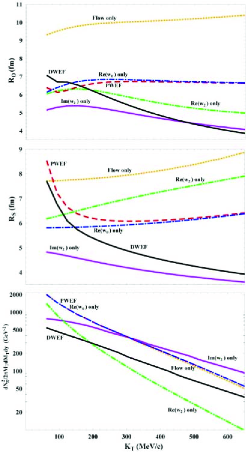
Figure 2: (Color online) Calculations of $R_{O}$, $R_{S}$, and spectrum, isolating potential and flow effects. DWEF (black solid) full calculation; PWEF (red dashed) plane wave calculation with no optical potential or flow; $Re(w_{2})$ only (green dot-dot-dash) calculation with no flow and only real part of momentum dependent optical potential ($w_{2}$); $Re(w_{0})$ only (blue dot-dash) calculation with no flow and only real constant optical potential ($w_{0}$); $Im(w_{2})$ only (solid violet) calculation with no flow and only imaginary part of momentum-dependent optical potential ($w_{2}$); Flow only (orange dotted) calculation with flow but no optical potential. Non-zero parameters in all calculations have the F193 values of Table I.

To illustrate the importance of the various effects of the DWEF model for computing the radii $R_{O},R_{S}$ and the spectrum, we have done calculations using the F193 fit parameters with various effects switched on separately. This is shown in Fig. 2. The curves labeled DWEF show the full calculation. Those labeled PWEF are computed using plane waves, i.e., the optical potential ($w_{0,2}$) and flow ($\eta_{F}$) are set to zero. The curves labeled $Re(w_{0})$ and $Re(w_{2})$ use only the real constant or momentum-dependent parts of the optical potential, respectively, set to the F193 values, with no flow. The curves labeled $Im(w_{2})$ use only the imaginary momentum-dependent part of the optical potential set to the F193 value, with no flow. Finally, the curves labeled $flow$ uses the F193 value of $\eta_{F}$, with no optical potential. All other parameters in these calculations are set to the F193 values of Table 1. This study indicates that both flow and the optical potential modify the HBT radii, but only the momentum dependent parts of the optical potential ($w_{2}$) affect the spectrum.

Figs. 3 and 4 show DWEF calculations using F193, as compared with the STAR data STARHBT ; STARspec used in the fit. We see that both the HBT radii and the spectrum (including the spectrum normalization) are reproduce very well indeed. However, some clarification is needed here on the issue of resonance pions. Our model describes only those “direct” pions that are emitted directly within the fireball and that participate fully in the HBT correlation. It does not predict the “halo” fraction of pions originating from resonance decays later in the process that will not participate in the HBT correlation (or that would make an unmeasurable “spike” in the correlation function near $q=0$). These latter pions are present in the measured spectrum and must be removed before fitting the spectrum with a DWEF calculation.

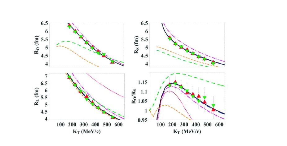
Figure 3: (Color online) HBT Radii $R_{s},R_{o},$, $R_{l}$ and the ratio $R_{o}/R_{s}$; Data STARHBT ): $\nabla$ (green) $\Rightarrow\pi^{+}\pi^{+}$; $\triangle$ (red) $\Rightarrow\pi^{-}\pi^{-}$. Curves: solid (black) $\Rightarrow$ full calculation; dotted (red) $\Rightarrow\eta_{f}=0$ (no flow); dashed (orange) $\Rightarrow$ Re$[U]$=0 (no refraction); dashed (green) $\Rightarrow$ $U$=0 (no potential); dot-dashed (blue)$\rightarrow,\;\mu_{\pi}=0$ (almost same as solid) double-dot-dashed (violet) $\Rightarrow$ substituting Boltzmann for Bose-Einstein thermal distribution.

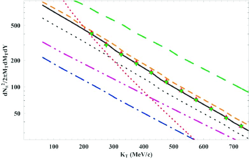
Figure 4: (Color online) Pion momentum spectrum. Data STARspec : $\nabla$ (green) $\Rightarrow\pi^{+}$; $\triangle$ (red) $\Rightarrow\pi^{-}$. Black dotted line is the ‘non-resonant pion” spectrum used in the fit. The curves are denoted as in Fig. 3.

We have done this by using the HBT $\lambda$ parameter previously extracted as part of the HBT analysis, which we take to represent the probability that both correlated pions are direct rather than halo pions. We fit the extracted $\lambda$ parameter with a straight line in transverse momentum to obtain the function $\lambda(p_{T})$. Then we remove the 12% weak decay correction of the published pion spectrumSTARspec and multiply it by $\sqrt{\lambda(p_{T})}$, thereby producing an estimate of the momentum spectrum of direct pions only. This corrected spectrum, as indicated by the black small-dashed line in Fig. 4, is then used in the data fitting. Following the DWEF calculation, the predicted theoretical spectrum is “uncorrected” by dividing it by $\sqrt{\lambda(p_{T})}$ and then reducing it by 12%, so that it can be compared directly with the published data. These predictions, now including halo pions, are the curves shown in the spectrum plots. We note that the effects of the two corrections to the spectrum tend cancel each other, and that their net effect on the fits is primarily an increase in temperature and flow parameters. We note also that the Phobos Collaboration has published spectrum data in the low $p_{T}$ regionBack:2004uh , but because the value of $\lambda$ in this region are not known, we cannot make similar corrections and therefore have not included these data in our current analysis. The DWEF fit parameters, particularly the temperature, flow, chemical potential, and Woods-Saxon diffuseness, are sensitive to the details of our treatment of resonances, thus introducing a procedure-dependent systematic error in DWEF parameter extraction.

Our DWEF calculations predict the correlation function of two pions with a particular vector momentum difference ${\bf q}$. There are at least two ways of extracting HBT radii from such correlation functions. One is to use the quadratic form (24) of the correlation function at very small magnitudes of ${\bf q}$. The other is to use the Gaussian form (23) at larger values of ${\bf q}$ that correspond to the falloff region of the correlation function. In our previous publicationCramer:2004ih we used the former method with $q=K_{T}/40$, a technique which essentially extracts HBT radii from the calculated curvature of the correlation function near $q=0$. In the present work we use the Gaussian form with $q=0.15$ fm^-1, a momentum difference that evaluates the correlation function near its half-maximum point, a procedure that bears more resemblance to the extraction of radii from experimental data with Gaussian fitting. We have found that in the medium and high momentum regions the two procedures gives very similar descriptions of the data and extract similar radii. However, we have found that for values of $K_{T}<175$ MeV/c, the two methods diverge, and that the Gaussian form gives more reliable radii.

IX.2 Wave Function Plots

We can understand more about how HBT measurements in various momentum regions probe the system under study by examining the computed wave functions from the DWEF calculation. Such wave functions calculated with the F193 fit are shown in Fig. 5. The complete DWEF wave functions (left column) differ significantly from the semi-classical eikonal approximation calculated with the same absorption (right column) at each of the energies we consider. The importance of the real part of the optical potential is illustrated by comparison with the center column, showing wave functions calculated with the real part of the optical potential set to zero. The maxima and minima of these plots result from interference effects caused by the optical potential as incorporated by solving the quantum mechanical wave equation. Their spacing gives a qualitative indication of the pion wavelength in the medium. The differences between the quantum calculations and the semi-classical eikonal model grow smaller as the value of $K_{T}$ increases. We note that while the high momentum wave functions sample only a “bright ring” at the edge of the fireball, the low momentum wave functions is also non-vanishing in most parts of the fireball.

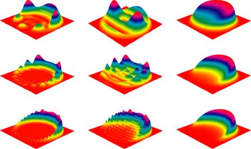
Figure 5: (Color online) Wave functions. The figures show the absolute square of the calculated wave functions times the density $\rho(b)$. For each (row) value of $K_{T}~{}(100,250,600)$ MeV/c, the full calculation, the calculation including only the imaginary part of the optical potential and the eikonal approximation with the same absorption are shown horizontally. The out direction is parallel to the lower right edge of each picture.

IX.3 Temperature Ambiguities

In our previous publicationCramer:2004ih the temperature parameter used in the pion emission function was $T=222$ MeV. This is an uncomfortably large value for the temperature of the medium, high enough that pions would be expected to “melt” in such an environment and lose their identity. Therefore, we explored (not shown) the extent to which the DWEF model requires such large values of temperature and showed that there is a parameter ambiguity involving the parameters $T$ and $a_{WS}$, such that a fit of reasonable quality could be obtained for temperature values over a fairly broad range.

Table 2: Nine Fit-Parameters Sets: These fits were obtained by fixing a range of values for the temperature $T$ and fitting the central Au+Au 200 GeV STAR data. Bold-face indicates a parameter fixed for the search.

Fit	$~{}~{}~{}~{}T$	$\eta_{f}$	$\Delta\tau$	$~{}R_{WS}$	$~{}a_{WS}$	$~{}~{}~{}w_{0}$	$~{}~{}~{}~{}~{}~{}w_{2}$	$\tau_{0}$	$\Delta\eta$	$~{}~{}~{}~{}\epsilon$	$\mu_{\pi}$	$\chi^{2}/DOF$
	$(MeV)$		$(fm/c)$	$~{}(fm)$	$~{}(fm)$	$(fm^{-2})$		$(fm/c)$			$(MeV)$
F173	173.0	1.451	2.664	11.924	0.541	0.095	0.777 +$i$0.112	8.77	0.983	0.000	139.57	2.81
F183	183.0	1.475	2.479	11.811	0.754	0.123	0.815 +$i$0.113	8.66	0.994	0.000	139.51	2.64
F193	193.0	1.507	2.382	11.773	0.909	0.139	0.847 +$i$0.120	8.60	0.991	0.000	139.57	2.45
F193a	193.0	1.508	2.380	11.773	0.912	0.139	0.850 +$i$0.121	8.62	0.987	0.0002	139.57	2.56
F193b	193.0	1.510	2.378	11.770	0.939	0.140	0.854 +$i$0.120	8.67	0.977	0.0137	139.57	2.56
F203	203.0	1.565	2.200	11.935	1.046	0.127	0.823 +$i$0.115	8.66	0.990	0.000	129.61	3.45
F203a	203.0	1.536	2.330	11.641	1.271	0.146	0.825 +$i$0.100	8.62	0.967	0.263	134.44	2.84
F213	213.0	1.577	2.323	11.689	1.330	0.131	0.817 +$i$0.101	8.54	0.970	0.296	129.54	3.16
F220	220.0	1.616	2.328	11.802	1.355	0.115	0.795 +$i$0.103	8.47	0.977	0.297	124.88	4.52

Therefore, it is desirable to choose a temperature appropriate to the medium. If one takes quite literally the expectation that the DWEF model describes the initial emission of pions and that the first pions are produced directly in the strongly interacting quark-gluon plasma as it make a phase transition to a hadronic phase, then the emission function should have the temperature of the QGP transition. Similarly, if the pions are produced as massless objects due to chiral symmetry restoration in the medium, then the chemical potential should equal the free pion mass. Recent lattice gauge calculations reported at Quark Matter 2005Katz:2005br give the critical QGP transition temperature to be 193 MeV. Therefore, we adopt (Table I) T=193 MeV and $\mu_{\pi}$=139.57 MeV and search for a new fit to the STAR $\sqrt{S_{NN}}$=200 GeV Au+Au data. To our surprise, the fit we obtain (see Figs. 3 and 4) with parameters fixed at these values is the best we have found, with an overall $\chi^{2}$ of 56.45 and a $\chi^{2}$ per degree of freedom of 2.45. Further, subsequent searches in which the fixed temperature was set to other values between 173 MeV and 220 MeV show that there is a definite minimum in $\chi^{2}$ at just the value of temperature given by the lattice gauge calculation. Table II shows nine different set of fit parameters, all of which give good fits to the central STAR $\sqrt{S_{NN}}$=200 GeV Au+Au data. In Table II, the fixed parameters are indicated in bold face. We see that F193, the parameter set of Table I, gives the best fit, and that for temperatures greater than 193 MeV it is necessary to use a non-zero value of $\epsilon$, invoking a Kisslinger-type wave equation Eq. (45), to obtain a quality fit. However, fits F193a and F193b indicate that searching on $\epsilon$ as part of a search at $T=$ 193 MeV gives values near zero and did not improve the fit.

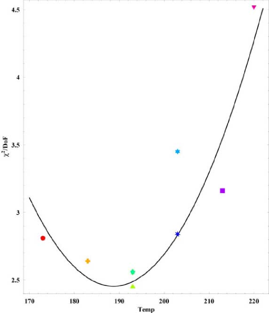
Figure 6: (Color online) Dependence of chi-squared per degree of freedom on temperature. Symbols correspond sequentially to the fits listed in Table II: circle (red), plus (orange), triangle (green), diamond (chartreuse), 5-star (aqua), 6-star (light blue), 7-star (dark blue), square (violet), and del (magenta). Black line is a parabolic fit to the points, provided to guide the eye.

Fig. 6 shows $\chi^{2}$ per degree of freedom as a function of temperature for the nine fits listed in Table II. The solid line is a parabolic fit to the points. We do not assert that there is physics driving the preference of the STAR data for the temperature predicted by lattice gauge calculations, but we believe this is more than a coincidence.

Fig. 7 shows the ratio of the parameters of Table II to the F193 parameters, and indicates the range of variations and the correlations of parameters. Note in particular the correlation between $T$, $a_{WS}$, $w_{0}$, $\Delta\tau$, and $\eta_{F}$.

Fig. 8 shows the predictions of all nine fits as compared with the STAR data. As can be seen, there are no striking differences. In order to make the differences more visible, Fig. 9 shows the ratio of the predictions of the eight other fits to those of F193. as c an be seen the differences in the radius predictions are less than 1%, while those of the spectrum predictions are as large as 10%.

However, we note that in the momentum region below 50 MeV/c, where no HBT or spectrum data is available, the different fits make different predictions. Fig. 10 shows the predictions of the fits of Table II in this region. We note that the “wiggles” arise mainly for the extreme fits, and in particular that these variations are relatively small for the F193 fit that provided the best fit to the higher momentum data.

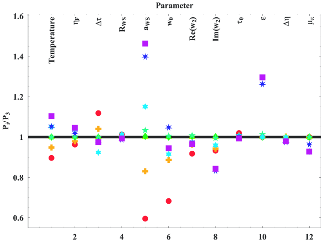
Figure 7: (Color online) Ratio of other fit parameters to those of F193 for the nine fits listed in Table II. Symbols correspond sequentially to the fits listed in Table II: circle (red), plus (orange), triangle (green), diamond (chartreuse), 5-star (aqua), 6-star (light blue), 7-star (dark blue), square (violet), and del (magenta).

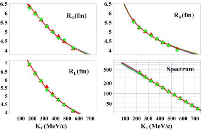
Figure 8: (Color online) Superposition of nine fits with STAR data, showing that there is relatively little difference between the predictions. Data points: $\nabla$ (green) $\Rightarrow\pi^{+}$; $\triangle$ (red) $\Rightarrow\pi^{-}$.

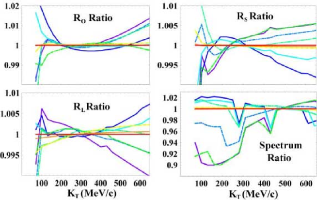
Figure 9: (Color online) Ratio of other predictions to F193. Colors correspond sequentially to the fits listed in Table II: red, orange, green, chartreuse, aqua, light blue, dark blue, violet, and magenta.

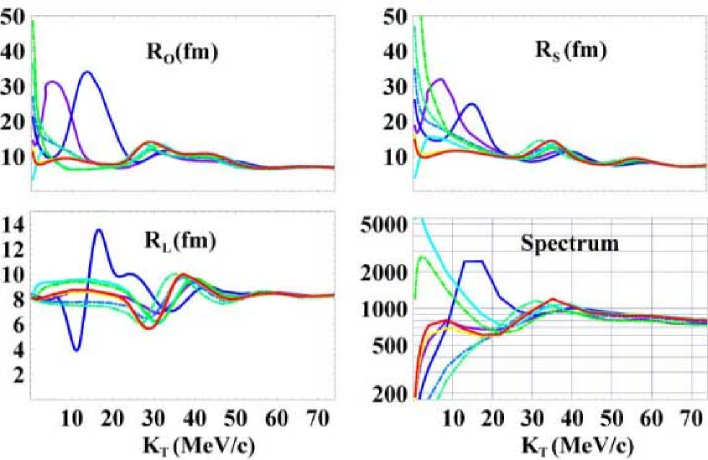
Figure 10: (Color online) Low-momentum predictions of the nine fits listed in Table II. Colors correspond sequentially to the fits listed in Table II: red, orange, green, chartreuse, aqua, light blue, dark blue, violet, and magenta. Note that the low temperature fits (red to aqua) have relatively little structure.

IX.4 Meaning of optical potential parameters

Table I shows that $w_{0}=0.14$ and that $w_{2}$ is 0.85 +0.12 i. Let us try to understand these values using the ideas of Sect. V. First consider the real parts. Comparing Eq. (45) and Eq. (44) shows that

$$w_{0}={m_{\pi}^{2}\over u_{\pi}^{2}}-m_{\pi}^{2}(T),\;\;{\rm Re}(w_{2})={1-u_{\pi}^{2}\over u_{\pi}^{2}}$$ (113)

which allows us to extract the values:

$$u_{\pi}^{2}=0.54,\;u_{\pi}=0.74,\;u_{\pi}m_{\pi}(T)=0.65\;{\rm fm}^{-1}.$$ (114)

These values are comparable to the estimates of Son:2002ci .

We also compare with the results of ShuryakShuryak:1991hb for pions propagating in hot dilute matter. His results for $T=200$ MeV (the stated limit of validity of the calculation) are most relevant for our case. His Fig. 1 shows results for $V=U/(2m_{\pi})$ as a function of pion momentum. The imaginary potential is approximately proportional to $p^{2}$ for $p\leq 400MeV/c$. For $p=1$ fm^-1 Shuryak obtains $Im(U)\approx 0.1$ fm^-2, which is close to our value of 0.12 fm^-2. Our real potential is about seven times larger in magnitude than our imaginary potential, while Shuryak finds that the strengths are comparable. Thus our real potential is much stronger than expected from a dilute gas approximation and consistent (via the formalism of Son:2002ci ) with the occurance of a chiral phase transition.

IX.5 Non-central Au+Au

Our analysis so far has focused on the central (0-5%) STAR $\sqrt{S_{NN}}$=200 GeV Au+Au data. However, the STAR collaboration performed measurements of pion correlations and spectra at $\sqrt{S_{NN}}$=200 GeV Au+Au as a function of centrality.

For non-central events, our optical potential would depend on the direction of ${\bf b}$ as well as its magnitude. The simple dependence on $b$ was exploited heavily in previous sections to simplify the calculations, so, in principle, non-cental collisions are not a part of our model. However, we can make simplifying assumptions that can allow us to predict the observables for non-central collisions. In particular, we assume that a non-central collision resembles a central collision with the same number of participants. This assumption allows us to extrapolate our results to systems that do not have perfect centrality by using participant scaling. In particular, we take the space-time parameters $R_{WS},a_{WS}$, and $\tau_{0}$ to scale as the centrality-dependent number of participant particles to the one-third power: $N_{\rm part}^{1/3}$. The values of $N_{\rm part}$ are taken from Glauber-model calculationsMillerthesis . For the Au+Au system, the value of $\Delta\tau$ is kept at the value of F193, because this is a dynamic quantity describing the proper-time duration during which pions are emitted in the collision. Table III gives the parameters $R_{WS},\tau_{0},a_{WS}$ and $\Delta\tau$ vs. centrality, as scaled from the F193 fit of Table I. Parameters not listed in the table are the same as those of Table I.

Table 3: Au+Au scaled space-time parameters from fit F193

$Centrality$	$~{}~{}~{}N_{\rm part}$	$~{}~{}~{}N_{\rm part}^{1/3}$	$R_{WS}$	$~{}~{}a_{WS}$	$\tau_{0}$	$\Delta\tau$
			$(fm)$	$(fm)$	$~{}~{}(fm/c)$	$(fm/c)$
0-5%	352.44	7.064	11.773	0.909	8.601	2.382
5-10%	299.31	6.689	11.149	0.860	8.145	2.382
10-20%	234.55	6.167	10.279	0.793	7.509	2.382
20-30%	166.68	5.503	9.173	0.708	6.701	2.382
30-50%	96.07	4.580	7.634	0.589	5.577	2.382
50-80%	29.75	3.099	5.164	0.398	3.773	2.382

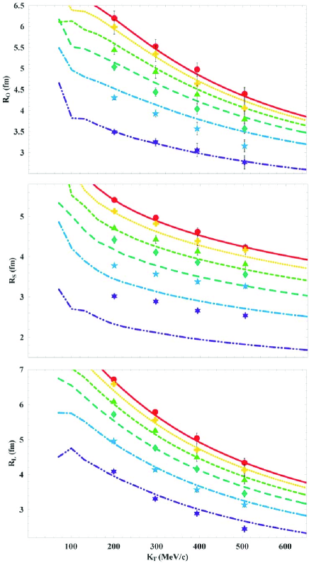
Figure 11: (Color online) Centrality dependence of HBT radii in Au+Au collisions. Curves are predictions from participant-scaled space-time parameters; data points are Au+Au at $\sqrt{s_{NN}}=200$ GeV from STARHBT . Symbols and colors: 0-5% circle (red), 5-10% plus (yellow), 10-20% triangle (green), 20-30% diamond (aqua), 30-50% 5-star (blue), 50-80% 6-star (indigo).

In Fig. 11 we see that the participant-scaled predictions work fairly well for the first few centrality bins, but agreement diminishes for the more peripheral collisions. We do not expect this simple scaling procedure to be accurate very far from the purely central collision assumption of the model, so this loss of predictive power is to be expected.

In particular, looking for differences between peripheral and central collisions is a standard way to test for the possible existence of QGP effects. This means that the strength of the optical potential parameters of our model should change as the collision becomes peripheral. We have kept the potential depth parameters constant with centrality because we have no way to predict their centrality dependence. Fig. 11 shows an excellent reproduction of $R_{L}$ with centrality, a fairly good reproduction of $R_{O}$, but only a fair description of $R_{S}$. We take this to be consistent with the disappearance of a chiral phase transition in the more peripheral collisions.

IX.6 Predictions for Cu+Cu collisions

The STAR collaboration has also measured (but not yet published) radii and spectra vs. centrality for Cu+Cu collisions at $\sqrt{S_{NN}}$=200 GeV, so it is of interest to make predictions for this system. Here again use participant scaling, but have also assumed that the emission duration parameter $\Delta\tau$ scales as $A^{1/3}$, where $A$ is that atomic mass number of the colliding nuclei. Table IV gives the scaled space-time parameters used to predict the HBT radii for the Cu+Cu system. Parameters not present in the table are the same as those of Table I.

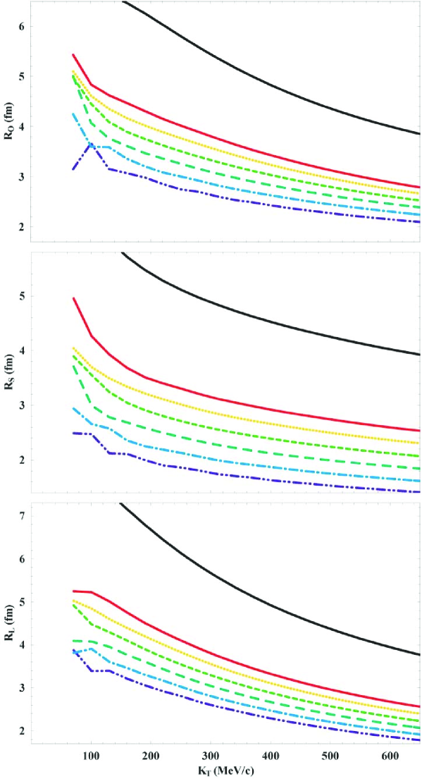
Figure 12: (Color online) HBT Radii: Central Cu+Cu ($\sqrt{s}=200$ GeV) predictions: Au+Au F193 fit - black solid; Cu+Cu Centrality 0-10% - red solid, 10-20% - yellow dot, 20-30% - green short-dash, 30-40% - aqua long-dash, 40-50% - blue dot-dash, 50-60% - violet dot-dot-dash.

Table 4: Cu+Cu scaled space-time parameters from fit F193

$Centrality$	$~{}~{}~{}N_{\rm part}$	$~{}~{}~{}N_{\rm part}^{1/3}$	$R_{WS}$	$~{}~{}a_{WS}$	$\tau_{0}$	$\Delta\tau$
			$(fm)$	$(fm)$	$~{}~{}(fm/c)$	$(fm/c)$
0-10%	98.38	4.616	7.694	0.594	5.621	1.629
10-20%	74.78	4.210	7.022	0.542	5.130	1.629
20-30%	54.37	3.788	6.314	0.487	4.613	1.629
30-40%	38.53	3.378	5.629	0.434	4.113	1.629
40-50%	26.29	2.974	4.956	0.382	3.621	1.629
50-60%	17.63	2.603	4.338	0.335	3.169	1.629

IX.7 Correlation functions and the Gaussian approximation

We apply the present formalism to obtain correlation function $C$ (with $\lambda=1$), using the parameters of Table I, for $K_{T}=158,316$ MeV/c. The results are shown in Figs. 13,14. We see that the correlation functions $C(K_{T},q)$ are fairly well represented by Gaussians, for the relevant range of small values of $q$, with widths that are approximately independent of $K_{T}$. For a typical radius of about 7 fm, and $q=0.15$ fm^-1, (where data are measured) $q^{2}R^{2}\approx 1$. Therefore, using the approximation (24) is not very accurate. On the other hand, the correlation functions are close to Gaussian in shape in this region, suggesting that approximation (23) is more appropriate. A detailed look at the ratio of computed correlation functions ($C-1$) to its Gaussian fit in Fig. 14 shows that the Gaussian curves represent the correlation functions fairly well in the region $0<q<0.22$ fm^-1 where $C-1$ is large and radii are extracted, but that the correlation functions are systematically larger than the Gaussian fit for $R_{O,L}$ and smaller for $R_{S}$ in the “tail” region ($q>0.22$ fm).

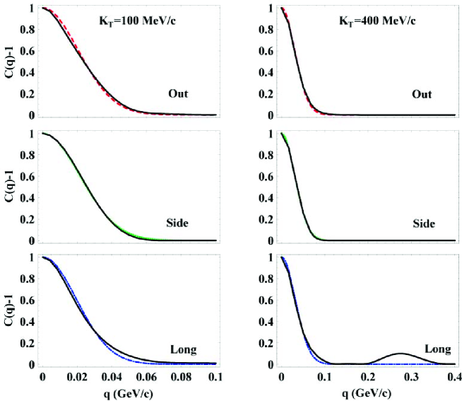
Figure 13: (Color online) Central Au+Au ($\sqrt{s}$=200 GeV). Correlation functions ($K_{T}$=158 , 316 MeV/c) for the out, side and longitudinal cases. The solid (black) curves are the full correlation functions. The broken curves are Gaussian fits: dash for out, dot for side and dot-dash for longitudinal.

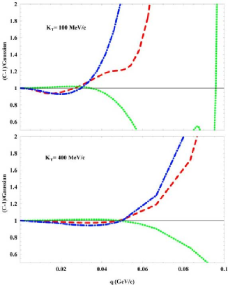
Figure 14: (Color Online) Central Au+Au ($\sqrt{s}$=200 GeV). Ratios of correlation functions ($K_{T}$=158, 316 MeV/c) to Gaussian fits for the out, side and longitudinal cases. The dashed (red) curves are obtained with ${\bf q}$ in the out direction, the dotted (green) curves with ${\bf q}$ in the side direction, and the dot-dashed (blue) curves with ${\bf q}$ in the longitudinal direction.

IX.8 Possible Extensions of the DWEF Model

The DWEF model presented here uses the empirical “hydrodynamics-inspired” emission function of Eq. (27). However, we note that the application of distorted waves to an emission function is more generally applicable, and that the formalism we present here can be applied to any emission function that has the same symmetry properties as Eq. (27). One extension of the model would be to calculate the emission function as a multi-dimensional numerical table directly from hydrodynamics and use this with the DWEF model to calculate spectra and radii. We also note that, while it has not been not implemented here, the DWEF model can allow the temperature and chemical potential to depend on $b$, as is done in the Buda-Lund model Buda . Preliminary investigations of this extension of the model, however, did not lead to an improved description of the data.

X The Eikonal Approximation

Several previous calculations Heiselberg:1997vh –Wong:2003dh of the effects of opacity have used the eikonal approximation to solve the wave equation (50). Here we explain the nature of this approximation and discuss its weaknesses and (fewer) strengths when applied to the current situation.

The basic idea is that if the momentum is large one may say approximately that the wave propagate in a given direction (here the out direction, which is taken as along the $x$ axis). Then one assumes a solution of the form ${\psi^{(-)}}^{*}({\bf b})=e^{ipx}\Phi({\bf b})$ that is inserted into the wave equation. Taking the Laplacian of the approximate wave function gives a term proportional to $p^{2}$ that is canceled, a term proportional to $p$ that is kept, and another term that is ignored. Then one finds

$${\psi^{(-)}}^{*}({\bf b}=x,y)=e^{ipx}\exp{\left[{-i\over 2p}\int_{x}^{\infty}U(x^{\prime},y)dx^{\prime}\right]}.$$ (115)

for propagation in the $x$ (out) direction. The corrections to this solution are of order ${-1\over 2iK}{1\over U}{\partial U\over\partial x}-{U\over 4K^{2}}$ times the terms that are kept. The first correction can be large in the surface region in which $U$ varies greatly and the second term can be large in the interior region in which $U$ reaches its full value. We are concerned with pions of momentum ranging from 30 to 600 MeV/c, so that the eikonal approximation be expected to be poor. However, the ease of application, and its wide use makes it worthwhile for us to assess the use of Eq. (115). We consider a purely imaginary potential first and then use a general complex potential.

X.1 Strong Absorption at High K – Purely Imaginary potential

In the impulse approximation $U=-4\pi f\rho$ where $f$ is the projectile-target scattering amplitude and $\rho$ is the density of scatterers. The optical theorem relates the imaginary part of $f$ to the total cross section $\sigma$ so that $Im[U]=-p\sigma\rho$. If we keep only the imaginary potential $-i/(2p)U=1/2\sigma\rho$ and for a constant density the intensity of the wave falls as $e^{-x\lambda_{\rm mfp}}$ with the mean free path, $\lambda_{\rm mfp}={1\over\sigma\rho}$. More generally the wave function for a purely imaginary optical potential is given by

$$\psi^{(-)}({\bf p}_{i},{\bf b})=e^{-i{\bf p}_{i}\cdot{\bf b}}e^{-l_{i}/2\lambda_{\rm mfp}}$$ (116)

where $i=1,2$ for the two wave functions and $l_{i}({\bf b},{\bf K})$ is the direct line path length (parallel to the direction of ${\bf p}_{i}$ from the emission point ${\bf b}$ to the edge of the medium. For a purely imaginary optical potential $U=-iK\sigma\rho$ and $\lambda_{\rm mfp}$ is the resulting mean free path.

Figure 15: Eikonal calculation of pion wave function. A pion produced at a position ${\bf b}$ propagates along a straight line path ${\bf l}$ until it hits the edge of the medium, denoted by ${\bf R}$. The angle between the dashed line and the horizontal line ${\bf l}$ is denoted in the text as $\theta$. The out case with $\theta_{s}=0$ is shown.

We have, see Fig. 15,

$${\bf R}={\bf l_{i}}+{\bf b},$$ (117)

$$R^{2}=l_{i}^{2}+b^{2}+2bl_{i}\cos{(\theta-\theta_{s})}.$$ (118)

$\theta$ is angle between ${\bf b}$ and $x$-axis (direction of ${\bf K}$) $\theta_{s}$ is angle between $\bf p_{1,2}$ and ${\bf K}$. This was called $\alpha$ in previous sections. The angle between ${\bf b}$ and ${\bf l_{i}}$ is $\theta-\theta_{s}$. Solving we find

$$l=-b\cos(\theta-\theta_{s})+\sqrt{(b\cos(\theta-\theta_{s}))^{2}+R^{2}-b^{2}}.$$ (119)

For the R-out case $\theta_{s}=0$, and

$$l_{i}=l=-x+\sqrt{R^{2}-y^{2}}$$ (120)

In this approximation the correlation function minus one is given by the absolute square of the ratio of integrals: ${I_{\parallel,\perp}(q)\over I_{\parallel,\perp}(q=0)}.$ In particular,

$$I_{\parallel}(q) = \int d^{2}be^{i{\bf q}\cdot{\bf b}}e^{-l/\lambda_{\rm mfp}},\quad{\bf q}\;\|\;{\widehat{{\bf x}}}$$ (121)

$$= {\lambda\over 1+iq\lambda}\int_{-R}^{R}dy\left(e^{iq\sqrt{R^{2}-y^{2}}}-e^{-(iq+2/\lambda_{\rm mfp})\sqrt{R^{2}-y^{2}}}\right).$$ (122)

If $\lambda_{\rm mfp}<<R$ we neglect the second term. Since we are interested in radii, we expand the remaining term in powers of the exponential (keeping $\lambda_{\rm mfp}<<R$):

$$I_{\parallel}(q)={\lambda_{\rm mfp}\over 1+iq\lambda_{\rm mfp}}\left(2R-q^{2}R^{2}/2(2R-2R/3)+iq\pi R/2\right)$$ (123)

$$C_{\parallel}(q)\approx 2-q^{2}R^{2}(2/3-\pi^{2}/16)$$ (124)

$$R_{O}^{2}=R^{2}(2/3-\pi^{2}/16)=0.0498R^{2};R_{O}=R/4.48$$ (125)

In the plane wave approximation (Eq. (122) with $\lambda_{\rm mfp}\to\infty$) one would find $R_{O}^{PW}=R/\sqrt{8}$. The striking result of Heiselberg & VischerHeiselberg:1997vh indicated that the measured radius should be 40% smaller than the radius obtained in plane wave approximation. This result is confirmed for the highest value of $K_{T}=3~{}{\rm fm}^{-1}\approx 600$ MeV/c by the calculations shown above in Fig. 2. The value of $R_{o}$ is reduced by approximately 40% by the influence of the imaginary optical potential. Fig. 16 shows the effects of increasing the imaginary potential (by varying $Im[w_{2}]$ from 0.1 to 0.5 in steps of 0.1). The computed value of $R_{O}$ does not change when $Im[w_{2}]$ is large enough and $K_{T}$ is high enough. Small deviations between our results for highest $K_{T}$ and the resultHeiselberg:1997vh can be attributed to the non-zero value of the diffuseness $a_{WS}$.

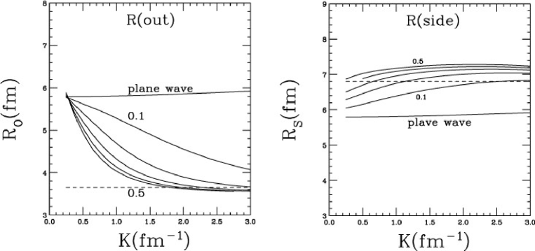
Figure 16: Radii $R_{o}$ and $R_{s}$ for increasing values of $Im[w_{2}]$. All other optical potential parameters and the flow parameters are set to 0. The numbers in the figure refer to the range of values. The dashed curve shows the result of Heiselberg & Vischer.

In the model of the present section, the correlation function and pion intensity would each be proportional to $\lambda_{\rm mfp}$, and a very small value would yield a very small pionic spectrum. More generally, the extraction of the chemical potential from the pionic spectrum depends on the mean free path parameter $\lambda_{\rm mfp}$.

Now let us do the R-side case. Then

$$\cos\theta_{s}={K\over\sqrt{K^{2}+q^{2}/4}};\sin\theta_{s}=\pm{q/2\over\sqrt{K^{2}+q^{2}/4}}$$ (126)

$$\cos{(\theta-\theta_{s})}=\cos\theta(1-{q^{2}\over 8K^{2}})\mp{q\over 2K}\sin\theta.$$ (127)

We find that

$$l_{i}\to-x+\sqrt{R^{2}-y^{2}}\pm{\cal O}({q\over K})+{\cal O}({q^{2}\over K^{2}})\approx-x+\sqrt{R^{2}-y^{2}}.$$ (128)

The terms $\pm{\cal O}({q\over K})$ cancel in computing the term $l_{1}+l_{2}$ that enters in computing the present correlation function. Thus the correction is of order $1/K^{2}$. The eikonal approximation works only if $KR\gg 1,$ so the corrections must be presumed to be small. Then

$$I_{\perp}(q)=\int_{-R}^{R}dye^{iqy}\int_{-\sqrt{R^{2}-y^{2}}}^{\sqrt{R^{2}-y^{2}}}dxe^{x/\lambda_{\rm mfp}}e^{-{1\over\lambda_{\rm mfp}}\sqrt{R^{2}-y^{2}}}$$ (129)

$$\approx\lambda\int_{-R}^{R}dy(1-q^{2}y^{2}/2)=\lambda_{\rm mfp}(2R-q^{2}R^{3}/3)$$ (130)

$$C_{\perp}(q)=2-q^{2}R^{2}/3$$ (131)

$$R_{s}^{2}=R^{2}/3,$$ (132)

Without distortion would be $C^{PW}_{\perp}(q)=2-q^{2}R^{2}/4$, so in this case the strong absorption increases the radius by a factor of $\sqrt{4/3}.$ This result is qualitatively obeyed in our realistic solutions of the wave equation, see Fig. 16.

X.2 Complex potential with non-vanishing real part

If there is an attractive real potential the wave function of Eq.(116) becomes:

$$\psi^{(-)}({\bf p}_{1},{\bf b})=e^{-i{\bf p}_{1}\cdot{\bf b}}e^{-l_{1}(1+i\alpha)/2\lambda_{\rm mfp}}$$ (133)

with $\alpha$ dimensionless, real and positive. If $\alpha=0$ one obtains the purely absorptive model of the previous sub-section. Conversely, the limit of a purely real potential occurs when $1/\lambda_{\rm mfp}\to 0,\alpha/\lambda_{\rm mfp}\to 1/\lambda_{0}$. We also have

$${{\psi}^{*}}^{(-)}({\bf p}_{2},{\bf b})=e^{i{\bf p}_{2}\cdot{\bf b}}e^{-l_{2}(1-i\alpha)/2\lambda_{\rm mfp}}$$ (134)

In the product $\psi_{{\bf p}_{1}}\psi_{{\bf p}_{2}}^{*}$ enters in computing the correlation function, so unlike the previous case of pure absorption, a term of the form $l_{1}-l_{2}$ enters. This difference is of order $q/K$ compared to other terms, but its influence in computing radii must lead eventually to a term of order $({q\over K})^{2}$. The validity of the eikonal approximation depends on the ability to disregard such terms. Thus a valid eikonal approximation means that $l_{1}=l_{2}$ so the factors of $\alpha$ cancel out in the product $\psi^{(-)}({\bf p}_{1},{\bf b}){{\psi}^{*}}^{(-)}({\bf p}_{2},{\bf b})$. Thus, if one assumes the eikonal approximation is valid at all values of $K_{T}$, one would find erroneously that the real potential never has an influence on the calculation of HBT radii.

Unlike the effects of the imaginary potential, which are qualitatively captured by the eikonal approximation (even if applied wrongly at low values of $K_{T}$), the effects of the real potential are completely lost. Thus the eikonal approximation can not be used for values of $K_{T}$ such that the real potential contributes. As shown in Fig. 3 the real potential is important for all values of $K_{T}$ less than 600 MeV/c. Conversely, for much larger values of $K_{T}$, for which the eikonal approximation does accurately reproduce the solution of the wave equation, the real potential will not play a role in determining radii.

XI Oscillations – a simple square well example

Our numerical results indicate that the radii may have significant oscillations for small values of $K_{T}=K$. The purpose of this sub-section is to provide a simple example that also yields oscillating radii. Consider a cylindrical source of radius $R$ of infinite extent in the longitudinal direction. Suppose this leads to a real, attractive square well potential of radius $R$ that is proportional to the square of the momentum, as motivated by Eq. (45). Then (50) becomes

$$(-\nabla^{2}-U_{0}p^{2})\psi=p^{2}\psi\qquad(b\leq R)$$ (135)

$$-\nabla^{2}\psi=p^{2}\psi\qquad(b>R),$$ (136)

with $U_{0}>0$. This equation is easily solved using the partial wave expansion (53). To provide a simple analytic example we further specify to the case of the lowest partial wave, $m=0$. In this case we find

$$\psi({\bf b})=J_{0}(p\sqrt{1+U_{0}}\;b),\qquad(b\leq R)$$ (137)

This shows immediately that the effect of the interaction is to scale each momenta $p_{1},p_{2}$ that appear in the wave functions by a factor $\sqrt{1+U_{0}}.$ We define

$$\widetilde{p}\equiv p\sqrt{1+U_{0}}.$$ (138)

Eq. (137) is a valid approximation to the full wave function (for $b\leq R$) only if $p\sqrt{1+U_{0}}R\ll 1$. However, it is interesting to also consider larger values of $p$.

To compute radii, recall the correlation function (69). For simplicity we take $\eta_{f}=0$, and consider fixed values of $\eta$ and $\tau$, with $\Delta\tau=0$. This corresponds to evaluating $S_{0}$ at its peak and neglecting the influence of time duration. In this case many factors in the numerator and denominator of Eq. (70) cancel. Then the correlation function is given by a simple expression that provides some insight:

$$C(K,q)-1=\frac{\phi^{2}_{R}(\widetilde{p_{1}},\tilde{p_{2}})}{\phi_{R}(\widetilde{p_{1}})\phi_{R}(\widetilde{p}_{2})}$$ (139)

$$\phi_{R}(p_{i},p_{j})\equiv{1\over R^{2}}\int_{0}^{R}bdbJ_{0}(p_{i}b)J_{0}(p_{j}b)=\frac{p_{i}\,J_{0}(p_{j}R)\,J_{1}(p_{i}R)-p_{j}\,J_{0}(p_{i}R)\,J_{1}(p_{j}R)}{R(p_{i}^{2}-p_{j}^{2})}$$ (140)

$$\phi_{R}(p_{i})\equiv{1\over R^{2}}\int_{0}^{R}bdbJ_{0}^{2}(p_{i}b)={1\over 2}\left(J_{0}^{2}(p_{i}R)+J_{1}^{2}(p_{i}R)\right)$$ (141)

If we are concerned with the side radius, inside the well $p_{1}=p_{2}=\sqrt{K^{2}+q^{2}/4}$ for the arguments of $J_{0}$ that enter. In that case, $\phi_{R}(p_{1},p_{2})\to\phi_{R}(p_{1},p_{1})=\phi_{R}(p_{1})$ and the correlation function takes on the value of 2 and the side-radius vanishes. This is a specific consequence of the approximation of taking only $m=0$–all directions of ${\bf K}$ are equivalent, so there is no influence of vectors ${\bf q}$ that are perpendicular to ${\bf K}$.

The out case is more interesting because the energies and magnitudes of momenta $p_{1,2}=(K\pm q/2)$ of the two pions are different. A non-zero radius is obtained by evaluating $C(K,q)$ for very small values of $q$ and using Eq. (26). The quantity $R_{O}(K)/R$ is displayed in Fig. 17.

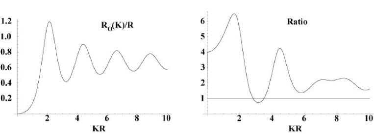
Figure 17: $R_{O}(K)/R$ and the ratio of eq (142). The parameter $U_{0}=1$.

We see that an oscillatory pattern similar to our realistic results, such as Fig. 3 for small values of $K_{T}$, emerges from the present calculation. This occurs simply because Bessel functions oscilate. Indeed the out-radius obtained without the influence of final state distortions ($U_{0}=0$) also has oscillations, but with a different frequency. Therefore another quantity of interest is the ratio of radii computed with $R_{O}(K)$ and without $R^{0}_{O}(K)$ the influence of distortions:

$${R_{O}(K)\over R_{O}^{0}(K)}\equiv\;{\rm Ratio}$$ (142)

displayed in Fig. 17. The oscillations seen in the right part of Fig. 17 demonstrate the significance of final state interactions that cause enhancements by factors of greater than six and suppressions by factors of 2! Furthermore, comparing the left and right hand sides of the figure shows the quantity $R^{0}_{O}(K)/R$ also oscillates. This is caused by the sharp edge of the square well and because we limit ourselves to $m=0$.

XII Summary

A complete formal treatment of the distorted waves treatment of HBT correlations is presented here. The need for incorporating the influence of an optical potential $U$ and the resulting distorted wave emission function is explained. The partial wave formalism necessary to compute the pionic distorted waves and the resulting emission function is detailed. Two different methods with equivalent results to evaluate the necessary eight-dimensional integral are described. Chiral symmetry restricts the form of $U$ boy ; Son:2002ci at low energy and the necessary constraints are implemented here and in Cramer:2004ih . An excellent description of the STAR Au+Au HBT and spectrum data is achieved for central collisions and the use of an average area formulation leads to a very good description of these observables for non-central collisions. We also use four different versions of geometrical scaling to predict the results of central Cu+Cu collisions. The ability to calculate the absolute magnitude of the spectrum as well as the radii Eq. (25),Eq. (26) (which involve ratios of functions of emmission functions) required for the computation of radii is a principal advantage of our method. The Blast Wave Model is discussed in Sec. IV.

The above results are achieved using a temperature $T_{c}$ fixed at the recently determined critical value of 193 MeV Katz:2005br . Such a value could present difficulties for conventional calculations of the spectra because chemical equilibrium analyses yield lower temperatures $T_{ch}=174$ MeV Braun-Munzinger:2001ip . A large difference between $T_{c}$ and $T_{ch}$ implies that the hadrons interact after the deconfinement transition occurs. This notion is entirely consistent with our treatment of pionic distortions which has as its fundamental assumption that pions interact in a hot dense medium before escaping to freedom.

We find that the necessary real optical potential is so strongly attractive that the pion can be said to lose its mass inside the medium. That chiral symmetry seems to be restored is the conclusion of our earlier workCramer:2004ih . The RHIC-HBT puzzle is therefore replaced by the need to investigate this restoration.

Explicit evaluation of wave functions obtained by exact numerical solutions of the wave equation show some interesting features of the strong interaction and also display differences with the solutions obtained using the eikonal approximation. A critical discussion of the eikonal approximation as applied to computing HBT radii shows that its use causes the crucial influence of the real part of the optical potential to be entirely lost. The huge importance of the real part of the optical potential is explicitly illustrated through a simple

There are many immediate applications of this formalism. In particular, a treatment of HBT data obtained at all energies is in progress and will be presented elsewhere.

Appendix

Consider the integral appearing in Sect. VIII.1:

$$f(\beta,\Delta\eta)=\int_{-\infty}^{\infty}d\eta\exp{(-\eta^{2}/(2\Delta\eta^{2}))}\cosh{(\eta)}\exp{\left({-\beta}\cosh{\eta}\right)},$$ (143)

that can be approximated Retiere:2003kf using Eq. (73)as

$$f(\beta,\Delta\eta)=2\exp{({1\over\Delta\eta^{2}})}K_{1}(\beta+{1\over\Delta\eta^{2}}).$$ (144)

Figure 18 shows that the approximation is excellent.

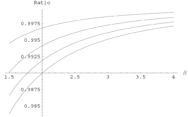
Figure 18: The ratio of the approximate expression Eq. (144) to the exact one of Eq. (143). The values of $\gamma$ range from .05 to 0.2, with ratio approaching unity as $\gamma$ approaches 0.

References

- (1) S. Pratt, “Two Particle And Multiparticle Measurements For The Quark - Gluon Plasma,” in Hwa, R.C. (ed.): Quark-gluon plasma, vol.2, page 700-748, 1995.
- (2) U. A. Wiedemann and U. W. Heinz, Phys. Rept. 319, 145 (1999).
- (3) P. F. Kolb and U. Heinz, Quark Gluon Plasma 3, edited by R.C. Hwa and X.-N. Wang, World Scientific, Singapore, 2004)
- (4) M. Lisa, S. Pratt, R. Soltz and U. Wiedemann, arXiv:nucl-ex/0505014.
- (5) S. Pratt, Phys. Rev. Lett. 53, 1219 (1984). G. F. Bertsch et al., Phys. Rev. C37, 1896 (1988).
- (6) D. H. Rischke and M. Gyulassy, Nucl. Phys. A 608, 479 (1996)
- (7) C. Adler et al. [STAR Collaboration], Phys. Rev. Lett. 87, 082301 (2001); K. Adcox et al. [PHENIX Collaboration], Phys. Rev. Lett. 88, 192302 (2002); A. Enokizono [PHENIX Collaboration], Nucl. Phys. A 715, 595 (2003).
- (8) U. W. Heinz and P. F. Kolb, hep-ph/0204061.
- (9) M. Gyulassy and L. McLerran, Nucl. Phys. A 750, 30 (2005).
- (10) J. G. Cramer, G. A. Miller, J. M. S. Wu and J. H. S. Yoon, Phys. Rev. Lett. 94, 102302 (2005); Phys. Rev. Lett. 95, 139901(E) (2005).
- (11) S. D. Katz, arXiv:hep-ph/0511166.
- (12) P. Braun-Munzinger, D. Magestro, K. Redlich and J. Stachel, Phys. Lett. B 518, 41 (2001)
- (13) E. V. Shuryak, Phys. Lett. B 44, 387 (1973).
- (14) M. Gyulassy, S. K. Kauffmann and L. W. Wilson, Phys. Rev. C 20, 2267 (1979).
- (15) J. I. Kapusta and Y. Li, arXiv:nucl-th/0503075.
- (16) T. Csörgő, B. Lörstad, and J. Zimányi, Z. Phys. C 71, 491 (1996).
- (17) T. Csörgő and B. Lörstad, Phys. Rev. C 54, 1390 (1996)
- (18) U. Heinz, in: Correlations and Clustering Phenomena in Subatomic Physics, edited by M.N. Harakeh, O. Scholten, and J.H. Koch, NATO ASI Series B, (Plenum, New York, 1997) (Los Alamos eprint archive nucl-th/9609029)
- (19) B. Tomasik and U. W. Heinz, Eur. Phys. J. C 4, 327 (1998) [arXiv:nucl-th/9707001].
- (20) F. Cooper and G. Frye, Phys. Rev. D 10, 186 (1974).
- (21) J. D. Bjorken and S. D. Drell, Relativistic Quantum Fields (McGraw-Hill, New York, 1965).
- (22) U.A. Wiedemann, P. Scotto and U. Heinz, Phys. Rev. C53, 918 (1996)
- (23) F. Retiere and M. A. Lisa, Phys. Rev. C 70, 044907 (2004)
- (24) L. S. Kisslinger Phys. Rev. 98, 761 (1955)
- (25) M. Csanad, T. Csörgő, B. Lorstad and A. Ster, J. Phys. G 30, S1079 (2004); T. Csörgő and B. Lorstad, Phys. Rev. C 54, 1390 (1996); M. Csanad, T. Csörgő and B. Lorstad, Nucl. Phys. A 742, 80 (2004).
- (26) J. Adams, et al. [STAR Collaboration], Phys. Rev. C 71, 044906 (2005)
- (27) M. Gell-Mann, R. J. Oakes and B. Renner, Phys. Rev. 175, 2195 (1968).
- (28) G. E. Brown and M. Rho, Phys. Rev. Lett. 66, 2720 (1991).
- (29) V. Koch, Prepared for International Summer School on Correlations and Clustering Phenomena in Subatomic Physics, Dronten, Netherlands, 5-16 Aug 1996 V. Koch, Int. J. Mod. Phys. E 6, 203 (1997).
- (30) D. T. Son and M. A. Stephanov, Phys. Rev. D 66, 076011 (2002) D. T. Son and M. A. Stephanov, Phys. Rev. Lett. 88, 202302 (2002)
- (31) D. Boyanovsky, H. J. de Vega and S. Y. Wang, Nucl. Phys. A 741, 323 (2004).
- (32) G. A. Baker, B. G. Nickel and D. I. Meiron, Phys. Rev. B 17, 1365 (1978).
- (33) C. Sasaki, Prog. Theor. Phys. Suppl. 156, 174 (2004)
- (34) J. Adams, et al. [STAR Collaboration], Phys. Rev. Lett. 92, 112301 (2004).
- (35) S. V. Akkelin and Y. M. Sinyukov, arXiv:nucl-th/0310036.
- (36) B. B. Back et al., Phys. Rev. C 70, 051901 (2004).
- (37) E. V. Shuryak, Nucl. Phys. A 533, 761 (1991).
- (38) M. Miller, Yale University, Ph.D. Thesis 2001 “Measurement of Jets and Jet Quenching at RHIC”
- (39) C. W. De Jager, H. De Vries and C. De Vries, Atom. Data Nucl. Data Tabl. 36, 495 (1987).
- (40) S. Chapman, P. Scotto and U. W. Heinz, Phys. Rev. Lett. 74, 4400 (1995).
- (41) H. Heiselberg and A. P. Vischer, Eur. Phys. J. C 1, 593 (1998).
- (42) M. C. Chu, S. Gardner, T. Matsui and R. Seki, Phys. Rev. C 50, 3079 (1994) [arXiv:nucl-th/9408005].
- (43) B. Tomasik and U. W. Heinz, arXiv:nucl-th/9805016.
- (44) C. Y. Wong, J. Phys. G 29, 2151 (2003).