Dynamics of $K^{+}$ Production in Heavy Ion Collisions close to Threshold

Abstract

In this article the production of $K^{+}$ at energies close to the threshold is studied in detail. The production mechanisms, the influence of in-medium effects, cross sections, the nuclear equation of state and the dynamics of the nucleons on the kaon dynamics are discussed. A special regard will be taken on the collision of Au+Au at 1.5 GeV, a reaction that has recently been analyzed in detail by experiments performed by the KaoS and FOPI collaborations at the SIS accelerator at GSI.

I Introduction

Kaons are pseudoscalar mesons containing strangeness. Strangeness is a property of some baryons and mesons which at their discovery had ‘strange’ long lifetime compared to the nuclear resonances known at that time. The quark model explained that property by the content of a strange (anti)quark. Normal nuclear matter - protons, neutrons and (following the old Yukawa idea) pions - are build up by two types of quarks, the so-called up- and down quarks. A further quark the so-called strange quark allows the description of the novel particles, as it can be seen in fig. 1.

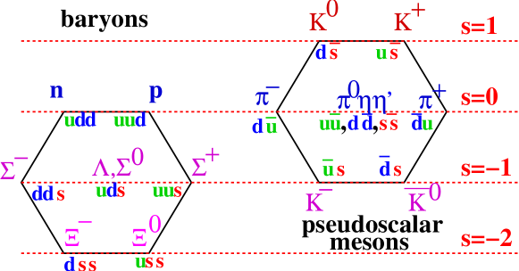
Figure 1: The basic SU(3) multipletts for baryons and pseudoscalar mesons

In the following time further particles giving need for new quark flavors were discovered. Today six quark flavors are assumed: up, down, strange, charm, bottom and top. These quarks are stable concerning the strong interaction, so that the whole net number of quarks of each flavor is conserved. Anti-quarks are counted with an opposite sign, so that the production of new particles via the production of quark-antiquark-pairs and rearrangement of the other quarks is possible. The conservation of the net quark numbers led to several conservation numbers like the strangeness content $S$

$$S=\sum\bar{s}-\sum s$$ (1)

Similarly, the charm quantum number describes the number of charm quarks etc. The net numbers of up and down quarks did not give rise to special conservation quantity since their conservation is implicitly assured by the conservation of the net baryon number and the charge.

However, the quark numbers are not stable against the weak interaction. Thus, a kaon may decay within about $10^{-8}$s into lepton pairs or mesons, e.g. $K^{+}\to\mu^{+}\bar{\nu}$. This effect is, however, important for the experimental detection but will not touch our theoretical considerations.

The interest of the kaon itself in a heavy ion collision is that during this short reaction time of about $10^{-22}$s strangeness is rigidly conserved and a produced $K^{+}$ can effectively not be destroyed. Thus, strangeness is a direct signal from a heavy ion reaction. This property has triggered for a long time a full spectrum of theoretical and experimental activities, whose exhaustive description would be quite impossible. For first ideas see for example dowa ; aik ; RanKo ; Barth ; Ahle ; schaffi ; cassing ; koli

In this article the production of kaons in relativistic heavy ion collisions at energies close to the threshold of elementary production is studied. This energy domain corresponds to experiments performed at the SIS accelerator at GSI (Darmstadt, Germany). This article focus on the positively charged $K^{+}$ which is better accessible by experiment. The $K^{0}$ is assumed to have similar properties. However, there is no unique relation to experiment, since the $K^{0}$ and its antiparticle, the $\bar{K^{0}}$, mix together into the short living $K^{0}_{S}$ and the long-living $K^{0}_{L}$. The antikaons ($K^{-}$ and $\bar{K^{0}}$) are not discussed neither, although their production is strongly coupled to the kaon production. Its exhaustive discussion would drastically enhance the size of this article. A special attention will be paid to the reaction Au+Au at 1.5 AGeV incident energy which has been recently investigated in detail by the KaoS and FOPI collaborations at GSI.

II Microscopic description of heavy ion collisions within IQMD

The Isospin Quantum molecular dynamics model (IQMD) ha89 ; hart ; baprc ; iqmd is a semi-classical model which describes heavy ion collisions on an event by event basis. Only a brief sketch of the model will be given here. For a detailed description see hart ; iqmd . For microscopic models of heavy ion collisions in general see st86 ; cas90 ; ai91 . For some review dedicated to strangeness production see urqmd .

II.1 Potentials in IQMD

In IQMD particles are represented by the 1 particle Wigner density.

$$f_{i}(\vec{r},\vec{p},t)=\frac{1}{\pi^{3}\hbar^{3}}{\rm e}^{-(\vec{r}-\vec{r}_{i}(t))^{2}\frac{2}{L}}{\rm e}^{-(\vec{p}-\vec{p}_{i}(t))^{2}\frac{L}{2\hbar^{2}}}$$ (2)

The total 1 particle Wigner density is the sum of all nucleons. The expectation value of the total Hamiltonian is

$$\langle H\rangle = \langle T\rangle+\langle V\rangle$$ (3)

$$= \sum_{i}\frac{p_{i}^{2}}{2m_{i}}+\sum_{i}\sum_{j>i}\int f_{i}(\vec{r},\vec{p},t)\,V^{ij}f_{j}(\vec{r}\,^{\prime},\vec{p}\,^{\prime},t)\,d\vec{r}\,d\vec{r}\,^{\prime}d\vec{p}\,d\vec{p}\,^{\prime}\quad.$$

The baryon-potential consists of the real part of the $G$-Matrix which is supplemented by the Coulomb interaction between the charged particles. The former can be further subdivided in a part containing the contact Skyrme-type interaction only, a contribution due to a finite range Yukawa-potential, and a momentum dependent part.

$$V^{ij} = G^{ij}+V^{ij}_{\rm Coul}$$

$$= V^{ij}_{\rm Skyrme}+V^{ij}_{\rm Yuk}+V^{ij}_{\rm mdi}+V^{ij}_{\rm Coul}+V^{ij}_{sym}$$

$$= t_{1}\delta(\vec{x}_{i}-\vec{x}_{j})+t_{2}\delta(\vec{x}_{i}-\vec{x}_{j})\rho^{\gamma-1}(\vec{x}_{i})+t_{3}\frac{\hbox{exp}\{-|\vec{x}_{i}-\vec{x}_{j}|/\mu\}}{|\vec{x}_{i}-\vec{x}_{j}|/\mu}+$$

$$t_{4}\hbox{ln}^{2}(1+t_{5}(\vec{p}_{i}-\vec{p}_{j})^{2})\delta(\vec{x}_{i}-\vec{x}_{j})+\frac{Z_{i}Z_{j}e^{2}}{|\vec{x}_{i}-\vec{x}_{j}|}+$$

$$t_{6}\frac{1}{\varrho_{0}}T_{3}^{i}T_{3}^{j}\delta(\vec{r}_{i}-\vec{r}_{j})$$

In the description of the Coulomb interaction $V^{ij}_{\rm Coul}$, $Z_{i},Z_{j}$ are the charges of the baryons $i$ and $j$.

The momentum dependence $V_{\rm mdi}^{ij}$ of the $N$–$N$ interaction, which may optionally be used in QMD, is fitted to experimental data ar82 ; pa67 on the real part of the nucleon optical potential ai87b ; bert88b , which yields

$$U_{mdi}=\delta\cdot\mbox{ln}^{2}\left(\varepsilon\cdot\left(\Delta\vec{p}\right)^{2}+1\right)\cdot\left(\frac{\rho_{int}}{\rho_{0}}\right)$$ (5)

The asymmetry energy is taken into account by the term

$$V^{ij}_{sym}=t_{6}\frac{1}{\varrho_{0}}T_{3}^{i}T_{3}^{j}\delta(\vec{r}_{i}-\vec{r}_{j})\quad t_{6}=100\,\rm MeV$$ (6)

where $T_{3}^{i}$ and $T_{3}^{j}$ denote the isospin $T_{3}$ of the particles $i$ and $j$, i.e. 1/2 for protons and -1/2 for neutrons.

The potential part of the equation of state resulting from the convolution of the distribution functions $f_{i}$ and $f_{j}$ with the interactions $V_{\rm Skyrme}^{ij}+V_{\rm mdi}^{i,j}$ (local interactions including momentum dependence) reads:

$$U\,=\,\alpha\cdot\left(\frac{\rho_{int}}{\rho_{0}}\right)+\beta\cdot\left(\frac{\rho_{int}}{\rho_{0}}\right)^{\gamma}+\delta\cdot\mbox{ln}^{2}\left(\varepsilon\cdot\left(\Delta\vec{p}\right)^{2}+1\right)\cdot\left(\frac{\rho_{int}}{\rho_{0}}\right)$$ (7)

The parameters $t_{1}...t_{5}$ are uniquely related to the corresponding values of $\alpha,\beta,\gamma,\delta$ and $\epsilon$ which serve as input. The standard values of these parameters can be found in table 1.

	$\alpha$ (MeV)	$\beta$ (MeV)	$\gamma$	$\delta$ (MeV)	$\varepsilon\,\left(\frac{c^{2}}{\mbox{GeV}^{2}}\right)$	$\kappa$ (MeV)
S	-356	303	1.17	—	—	200
SM	-390	320	1.14	1.57	500	200
H	-124	71	2.00	—	—	376
HM	-130	59	2.09	1.57	500	376
INT	-157	103	1.58	—	—	284
VH	-110	56	2.40	—	—	456

Table 1: Parameter sets for the nuclear equation of state used in the QMD model

In the calculations presented in this article the parametrization SM is used as standard. It is a combination of Skyrme type and momentum dependent potential with a low compressibility.

II.2 Collisions

Two particles collide if their minimum distance $d$, i.e. the minimum relative distance of the centroids of the Gaussians during their motion, in their CM frame fulfills the requirement:

$$d\leq d_{0}=\sqrt{\frac{\sigma_{\rm tot}}{\pi}},\qquad\sigma_{\rm tot}=\sigma(\sqrt{s},\hbox{ type}).$$ (8)

where the cross section is assumed to be the free cross section of the regarded collision type ($N-N$, $N-\Delta$, …).

The total cross section is the sum of the elastic cross section and all inelastic cross sections.

$$\sigma_{\rm tot}=\sigma_{\rm el}+\sigma_{\rm inel}=\sigma_{\rm el}+\sum_{\rm channels}\sigma_{i}$$ (9)

For instance for a pp collision we may have

$$\sigma_{\rm tot}=\sigma_{\rm el}+\sigma(pp\to p\Delta^{+})+\sigma(pp\to n\Delta^{++})$$ (10)

The cross sections for the different channels are given by experiment or by spin/isospin coefficients. For the pp case for example we have

$$\sigma(pp\to n\Delta^{++})=3\sigma(pp\to p\Delta^{+})=\frac{3}{4}\sigma_{\rm inelastic}$$ (11)

Inaccessible reactions like $\Delta N\to NN$ are calculated from their reverse reactions (here $NN\to\Delta N$) using detailed balance.

The possibility of reaching a channel in a collision is given by its contribution to the total cross section:

$$P_{\rm channel}=\frac{\sigma_{\rm channel}}{\sigma_{\rm tot}}\qquad{\rm e.g.}\quad P_{pp\to p\Delta^{+}}=\frac{1}{4}\frac{\sigma_{\rm tot}-\sigma_{\rm el}}{\sigma_{\rm tot}}$$ (12)

In the example we took use of eqns. 9, 10 and 11.

In the numerical simulation the choice of the channel is done randomly with the weight of the probability of the channel.

II.3 Virtual particles

The production of kaons in this energy domain is a very rare process. Their production cross section is only a few nanobarn. In comparison of a total cross section of about 20-40 mb the possibility of producing strangeness is very small. Therefore, the method presented a few lines above will cause severe statistical limitations to the description of kaons in this way. However, simulation codes oriented toward higher energies, like UrQMD urqmd apply successfully this method for reactions nearby the threshold. Their results (without optical potential) are quite comparable to IQMD results bleicher . A method to overcome this problem is the way of “perturbative production” of kaons, as it was for example done in kaon94 . In this method one only looks for the probabilities of producing a kaon in a collision (see eq. 12) and notes these reactions with their probability $P$, their cm-momentum $\vec{p}$ and their invariant mass $\sqrt{s}$. The collision itself continues normally (without kaon production) and later on the reactions are analyzed to estimate the properties of the kaons.

However, this method has the disadvantage that further interactions of the particles can only be roughly estimated. To overcome this we use the method of virtual particles:

• Each particle $i$ has a probability $P_{i}$. Protons, neutrons, deltas and pions start with $P_{i}=1$.

• After production of a new particle with a reaction probability $P_{r}$ the parents have a probability $(1-P_{r})$ for continuing undisturbedly. The produced particle has the probability $P_{n}=P_{1}\cdot P_{2}\cdot P_{r}$, where $P_{1}$ and $P_{2}$ are the probabilities of the parents.

• In the collision of two particles $i$ and $k$ with the probabilities $P_{i}$ and $P_{k}$, the final state of the collision will be calculated. Each particle will join this final state with the probability of his reaction partner:

  $$P(\mbox{\rm$i$ into final state})=P_{k}\qquad P(\mbox{\rm$i$ remains in prev. state})=1-P_{k}$$ (13)

• The interactions potentials are the interaction potentials of free particles multiplied by the probabilities of the interacting particles.

  $$V_{i}=\sum_{k}P_{k}V_{ik}$$ (14)

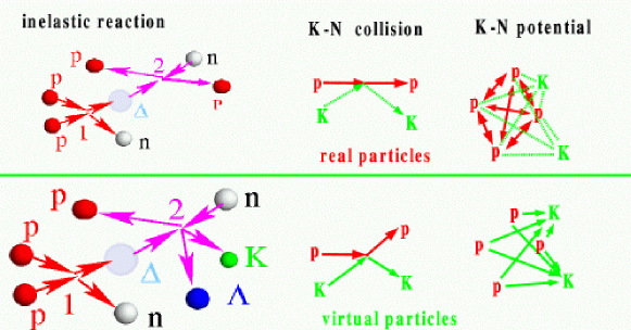
Figure 2: The major differences of “real” and “virtual” particles.

Since $P\ll 1$, $1-P\approx 1$, we can simplify the scheme in the following way.

• Nucleons, deltas and pions are real particles with $P=1$. Strange particles are virtual particles who have a very small probability $P_{i}$.

• In a collision virtual particles are produced with a reaction probability $P_{r}=\sigma({\rm Kprod})/\sigma(tot)$. The parent particles neglect this production and follow another channel of the collision according to its probability. (Fig. 2 , top-left).

  The produced particles act as if the production reaction had taken place and carry a probability of $P_{r}$ (Fig. 2 , bottom-left).

• In a collision of a real and a virtual particle, the real particle will ignore this reaction (Fig. 2 , top-middle). The virtual particle will act, as if this collision had taken place (Fig. 2 , bottom-middle).

• The real particles do not see a potential interaction with the virtual particles (Fig. 2, top-right). The virtual particles feel a potential with the nuclear matter (Fig. 2, bottom-right).

This method has the advantage to allow for high statistic calculation of kaon one-body observables including all effects of the medium like potential propagation, rescattering, absorption etc. However, there are some major drawbacks of this method

1. The energy conservation is no more assured on an exact level. Thus, the event characteristics of kaon producing events are identical to the characteristics of events without kaons. Questions like ‘Do events with kaons produce less high energetic pions than other events’ (which would be interesting for analogies between kaons and high energy pions) cannot be addressed.

2. KN- correlations cannot be performed since the event characteristic is not correct for kaon producing events.

3. Higher order processes might be described incorrectly. To give an example for a problematic description:

   1. A $NN$ collision produces virtually $N\Lambda K^{+}$. In the ‘real world’ it produces a $N\Delta$-pair.

   2. The virtual $\Lambda$ rescatters with another nucleon while the real $\Delta$ decays into $N\pi$.

   3. The virtual $\Lambda$ and the real $\pi$ resulting from the delta decay scatter and produce a $NK^{-}$-pair.

   The latter process should not be allowed since a real production of the $\Lambda$ would have avoided the $\Delta$-production and therefore the $\pi$ should not exist if the $\Lambda$ is there. This process is explicitly forbidden (by triggering on different parents of the collision partners) but it could be hidden by intermediate rescattering of a pion $\pi N\to\Delta\to\pi N$. However, its probability is rather low.

II.4 The KN-optical potential

The description of the KN-optical potential is a subject of vivid discussion. We use in our calculation a parametrization calculated by Jürgen Schaffner-Bielich schaffi which is derived from relativistic mean field (RMF) calculations and transformed into a Schrödinger-type potential of the following form:

$$U_{opt}^{K}=\sqrt{(\vec{k}-g_{v}\vec{\Sigma_{v}})^{2}+m_{K}^{2}+m_{K}g_{s}\Sigma_{s}}+g_{v}\Sigma_{v}^{0}-\sqrt{k^{2}+m_{K}^{2}}$$ (15)

The parametrization contains scalar fields ($g_{s}\Sigma_{s}$) which couple to the mass term and vector fields $g_{v}(\Sigma_{v}^{0},\vec{\Sigma_{v}})$ which couple to the momenta. The used parametrization is depicted on the l.h.s. of fig. 3.

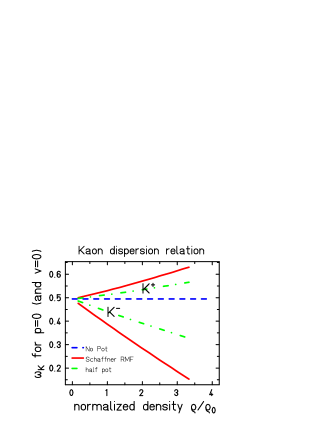
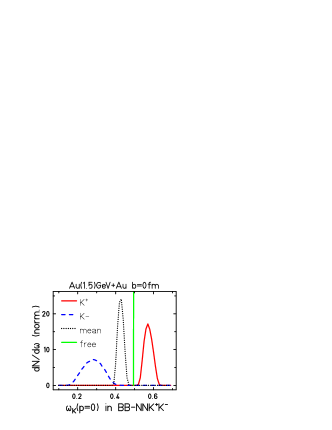
Figure 3: The used parametrization of the optical potential and its influence on the kaon production in $BB\to NNK^{+}K^{-}$ reactions in Au(1.5 AGeV)+Au collisions

We see that the potential (red full line) enhances the zero-momentum energy $\omega_{K}$ (which corresponds to an ‘in-medium mass’ ) for the $K^{+}$ and reduces it for the $K^{-}$ if the system becomes more dense. Without potential (blue dashed line) this energy corresponds exactly to the free kaon mass. Thus, the production of a $K^{+}$ will require more energy in a dense system. On the contrary, the production of a $K^{-}$ will require less energy. The curves reach the value of the free kaon mass if the density becomes small.

A calculation with reduced parameters (half pot, green dash-dotted line) will yield less significant changes and simulates a weaker strength of the optical potential.

The r.h.s of fig. 3 shows the application of the RMF optical potential to a calculation of a Au+Au head-on (b=0fm) collision at 1.5 AGeV. All baryonic collisions having sufficient energy for a $BB\to NNK^{+}K^{-}$ reaction are analyzed concerning the density where the collision takes place. The zero-energy of the $K^{+}$ (red full line) enhances by about 90 MeV, while the zero-energy of the $K^{-}$ (blue dashed line) is reduced by about 200 MeV. The average energy of both particles (black dotted line) is reduced by about 50-60 MeV. Thus, the threshold of this reaction will be reduced in the average by about 100 MeV.

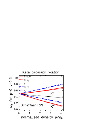
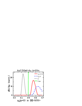
Figure 4: The contribution of scalar and vector part to the optical potential and its influence on the kaon production in $BB\to NYK^{+}$ reactions in Au(1.5 AGeV)+Au collisions

The used optical potential is a combination of scalar and vector potentials. The scalar part of the potential couples in the same way to $K^{+}$ and $K^{-}$ while the vector part couples to both particles with an inverted sign. Thus, the difference between $K^{+}$ and $K^{-}$ in fig. 3 is due to the vector part, while the lowering of the average energy of $K^{+}$ and $K^{-}$ (r.h.s.) is due to the scalar part. Fig. 4 shows on the l.h.s. the variations which occur, when instead of the full potential (red full line) only parts of the potential are used. If we only employ the scalar part (black dotted line) both $K^{+}$ and $K^{-}$ will show a lowering of the energy, which will be identical for both $K^{+}$ and $K^{-}$. The lowering of the $K^{-}$ is weaker than in the full combination of scalar and vector part. If we only use the vector parts (blue lines) the difference of $K^{+}$ and $K^{-}$ will remain but the energies will be quite higher for both $K^{+}$ and $K^{-}$. A reduction of the vector potential to the temporal part only $g_{v}\Sigma_{v}^{0}$ will slightly lower the energy. This effect depends on the relative velocity $v$ of the nuclear medium.

On the r.h.s. of fig. 4 the effect of the different parts on the $K^{+}$ production is shown. For a Au+Au head-on collision at 1.5 AGeV all baryon-baryon collisions with sufficient energy to produce a kaon (the lowest threshold is the threshold of the $BB\to NYK^{+}$ reaction) have been analyzed. A use of the scalar potential (black dotted line ) lowers the kaon energy and thus the threshold by about 70 MeV, while the vector potential only (blue dashed line) yields a strong enhancement. The full potential (red full line) shows an average enhancement of about 70 MeV. This value is slightly lower than the average value obtained from fig. 3 since the threshold for the reactions regarded here is lower than in fig. 3. For those reactions with lower thresholds the mean density of the collisions is lower.

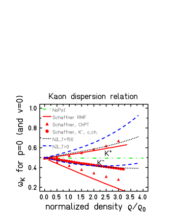
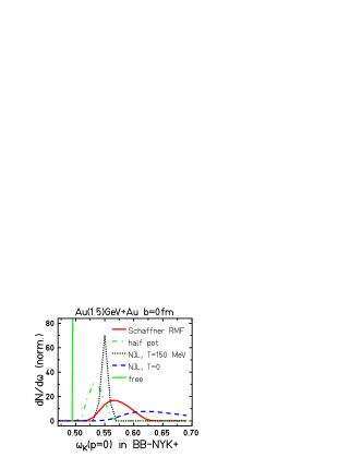
Figure 5: Comparison of the used parametrization of the optical potential to other parametrization and their influence on the kaon production in $BB\to NYK^{+}$ reactions in Au(1.5 AGeV)+Au collisions

Finally, fig. 5 compares the used optical potential (Schaffner RMF, red full line) to other calculations like Chiral Perturbation Theory (ChPT, red triangles) or calculation resulting from the Nambu-Jona-Lasinio model (NJL) using different assumptions for the temperature ($T=150$MeV, black dotted and $T=0$, blue dashed line). Except for the NJL, $T=0$ calculation the values for the $K^{+}$ are quite similar. However, the values for the $K^{-}$ differ visibly. In a Au+Au collision the different parametrization will yield different changes of the threshold (r.h.s.). Therefore, some observables might be different when using different potential parametrization. We will come to this point later on.

II.5 Dynamics of heavy ion collisions

In order to understand the dynamics of kaon production we want first to sketch rapidly the dynamics of the whole heavy ion collision in which the production and propagation of strange particles is embedded.

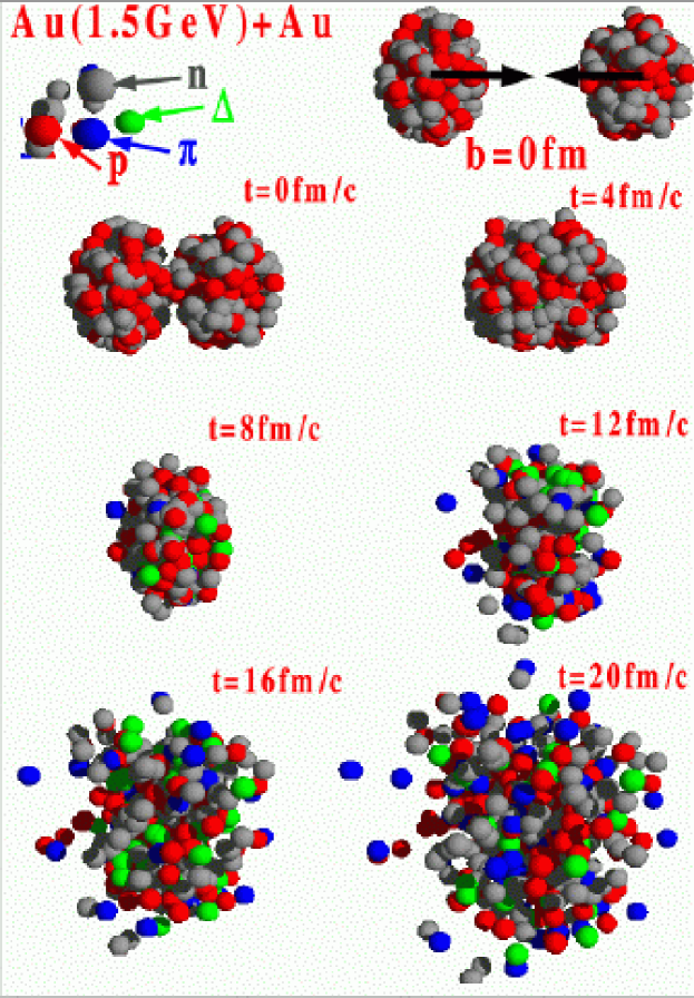
Figure 6: Time evolution of a Au(1.5AGeV)+Au collision at $b=0$ fm seen in coordinate space

Fig. 6 shows some ‘photos’ of a heavy ion reaction of Au+Au at 1.5 AGeV incident (lab) energy at an impact parameter of $b=0$fm. The scene is seen in the centre-of-mass frame. Therefore, the projectile and target approach each other in a symmetric way and both show a Lorentz contraction of their longitudinal size. Protons are shown as red balls while neutrons are shown as gray balls. The time of the whole reaction is very short (less than $10^{-22}$ seconds). Therefore, it is commonly used to measure the time in units of fm/c.

$$1\mbox{fm/c}=\frac{10^{-15}\mbox{m}}{3\cdot 10^{8}\mbox{m/s}}\approx 3\cdot 10^{-24}\mbox{s}$$ (16)

At $t=0$ fm/c projectile and target have first contact. First nucleon-nucleon collisions take place and first resonances are built up in the centre of the reaction. The nuclear matter starts to become stopped by inertial confinement and the density is increasing rapidly.

At about $t=4$ fm/c the production of resonances is strongly rising. However, they are mostly produced in the dense centre and not ‘visible’ from outward.

At about $t=8$ fm/c the system is reaching maximum density in the centre of the reaction. Nevertheless, the density in the peripheral region of the reaction is rather low. First resonances (deltas, green balls) reach the surface. Some of them decay into pions (blue balls).

At about $t=12$ fm/c the maximum number of deltas is reached. The system is still highly compressed. Most of the nucleons have collided and do no more carry the initial momentum. The spectra of the nucleons are highly non-thermal.

At about $t=16$ fm/c the pions have overtaken the dominance over the Deltas. The system is in expansion. The central density falls down rapidly.

At about $t=20$ fm/c the system is dominated by the expansion. The number of high energetic collisions drops strongly. There are still some deltas who will decay into nucleons and pions. The momentum distributions of the nucleons start to approach their final values.

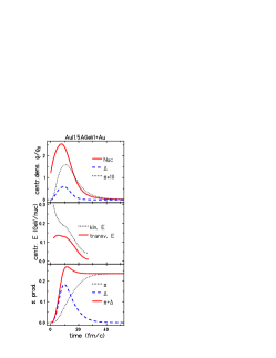
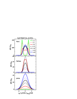
Figure 7: Time evolution of a Au(1.5AGeV)+Au collision at b=0fm. Left: Evolution of central density, central energy and pion number as function of time. Right: Evolution of the normalized rapidity distributions

Fig. 7 shows on the left hand side the time evolution of the density in the central region (top), the mean total and transverse energy in the central region (mid) and the number of deltas and pions (bottom). The nucleon density (top, red full line) grows up rapidly, reaches a maximum of about three times ground state density at about 8 fm/c and falls down afterward. The delta density (black dotted line) starts later, reaches a maximum of nearly half ground state density at about 9 fm/c and falls down rapidly. The pion density (multiplied by 10, blue dashed line) starts even later and reaches a maximum of around one sixth ground state density at about 10 fm/c.

In the central region the kinetic energy (middle, black dotted line) drops down rapidly. The incident energy in the centre-of-mass frame is due to the big longitudinal initial momentum. This energy is partly eaten up by the creation of resonances (deltas). Another part of the longitudinal momentum is redirected by nuclear collisions into the transverse direction. Therefore, the transverse energy (red full line) is built up rapidly in the central region. In the final expansion phase the fast (high energy) particles are leaving the central region quite rapidly, leaving the slower particles behind. The energies are falling down. Finally, the particles are leaving the central region.

The fast dropping of the energy in the mid-part of the lhs of fig. 7 is accompanied by a fast increase of the number of deltas (bottom, blue dashed line). As already stated, the resonances eat up a big amount of the energy. This energy will be released later on in form of pions (black dotted line). Their number is continuously increasing to reach the final number at about 30-40 fm/c. Pions are strongly interacting with nucleons. Therefore, pions decaying in the dense medium have a high chance to be reabsorbed and to refeed the number of deltas. This effect explains the slow increase of the pion number when the density is high. The deltas themselves can be reabsorbed by the nuclear matter. This effect can be seen when looking at the total number of deltas and pions (full red line). It shows a maximum at about 10-12 fm/c and decreases slightly afterward. After about 20 fm/c it stays roughly constant. Now only the contribution of deltas and pions to the total number is changing.

The right hand side of fig. 7 shows the time evolution of the rapidity distribution of nucleons (top), deltas (middle) and pions (bottom). The rapidity has been scaled to the projectile rapidity in the centre-of-mass. Thus, 1 corresponds to projectile rapidity, -1 corresponds to target rapidity.

At $t=0$ fm/c (green full line) projectile and target show their incident momenta as peaks at projectile and target rapidity. The broadening of the peaks is due to the Fermi momentum of the nuclei. Deltas and pions do not exist at this time.

At $t=4$ fm/c (red dotted line) first nucleons have been stopped to mid-rapidity. First deltas have been produced. The stopped nucleons collide with incoming nucleons of projectile and target causing a slight double peak of the delta rapidity distribution at about the middle of cm-rapidity (0) and projectile (1) resp. target rapidity (-1). There are nearly no pions.

At $t=8$ fm/c (red full line) when maximum density is reached, the nuclei have still not been completely stopped. There are still remnants of the peaks at projectile and target rapidities. The number of deltas has strongly increased. Its distribution is now peaked around mid-rapidity. The rather narrow width is due to the high mass of the delta which eats up a big part of the energy available in the first collisions. After the decay of the deltas a big amount of momentum is given to the light pions. Therefore, the rapidity distribution of them becomes quite broad.

At $t=12$ fm/c (black dashed line) the nucleon rapidity is peaked at mid-rapidity. The delta distribution shows its maximal values while the pion distribution rise up continuously.

At $t=16$ fm/c (full black line) and $t=20$ fm/c (blue dotted line) the nucleon rapidity distribution is slightly growing up in the centre. This is due to the feeding by the decay of the deltas whose rapidity distribution is continuously falling down. For kinematic reason the nucleon only gets few energy from the decay while most of the energy is given to the light pion whose broad rapidity distribution is still rising in number.

At $t=60$ fm/c (full blue line) the reaction is in the final state. There are no more deltas. The system is expanding and the particles will direct outward and finally touch the detectors.

II.6 Comparison to experiment

In the discussion of the kaon dynamics we will later on find a lot of cross talk between the nucleons and the kaons. Therefore we want first to assure that the dynamics described above is comparable to experiment. This will allow us as well to study some ingredients which may have some influence on the kaon production.

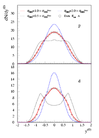
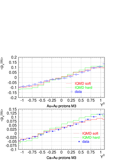
Figure 8: Comparison of IQMD calculations using different nucleon-nucleon cross sections to Ru+Ru data of FOPI (left) and comparison of Ca+Au and Au+Au flow data (right)

On the left hand side of fig. 8 we see a comparison of IQMD results with FOPI data performed by the FOPI collaboration hong on the system Ru+Ru at 400 AMeV incident energy. Here the rapidity distribution of protons (top) and deuterons (bottom) are studied. IQMD uses as cross section the free nucleon-nucleon cross sections $\sigma_{NN}^{free}$ (full line). The effect of the surrounding medium is taken into account by requiring the validity of the Pauli principle in the final state. In dense matter the cross section is effectively reduced. There is the possibility to apply additional factors the cross section as it is done on left hand side of fig. 8. A reduction of the cross section to half of the value ($0.5\times\sigma_{NN}^{free}$, dotted line) yields less stopping and a broader rapidity distribution while the doubling of the cross section ($1.0\times\sigma_{NN}^{free}$, dashed line) yields a smaller rapidity distribution. The data (circles) support an unscaled free cross section with Pauli blocking.

The right hand side of fig. 8 presents the comparison of transverse flow data of Au+Au and Ca+Au at 1.5 AGeV incident energy to IQMD results also performed by the FOPI collaboration hartmann . Here the influence of the nuclear equation of state is studied. The nuclear equation of state describes the repulsion of the nuclear matter against compression. A hard equation of state has a stronger repulsion and thus yields stronger transverse flow st86 while a soft equation of state causes less repulsion and less flow. The comparison seems to prefer the soft equation of state, an equation of state which will also be supported later on in the discussion of the influence of the equation of state to the kaon production. In general it can be stated that IQMD seems to describe the nucleon dynamics reasonably well.

II.7 Comparison of pion spectra

The dynamics of the pions is strongly coupled to the dynamics of the nucleons. The pions are produced in inelastic collision by the production of delta resonances. The delta decays into a nucleon and a pion. The pion has a high cross section of being absorbed by a nucleon. This absorption majorly creates a delta which may again decay into pion and nucleon. However, it may also be possible that the delta is reabsorbed in an inelastic collision with a nucleon. Thus, long chains of delta-nucleon-pion interactions of these types are possible hart :

$$\begin{array}[]{rcccccccl}NN&\to&N\Delta&&&&&&\\ &&N\Delta&\to&NN&&&&\\ &&\Delta&\to&N\pi&&&&\\ &&&&N\pi&\to&\Delta&&\\ &&&&&&N\Delta&\to&NN\\ &&&&&&\Delta&\to&N\pi\\ &&&&&&&&N\pi\to\ldots\\ \end{array}$$ (17)

One major ingredient in this dynamics is the delta decay width far off the pole. There are parametrizations of the lifetimes of deltas which differ especially at low delta masses. Some examples of them are given on the left hand side of fig. 9.

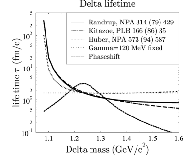
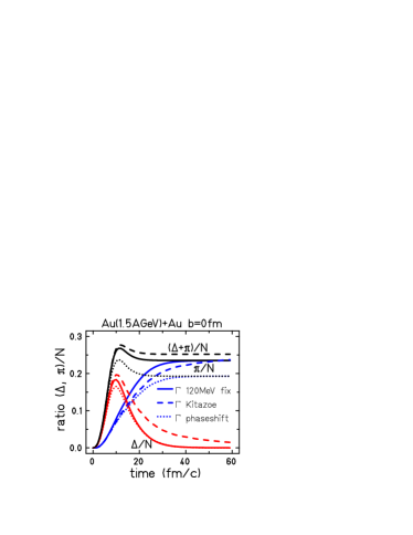
Figure 9: Different parametrizations of the delta lifetime (left) and their influence on the delta and pion time evolution (right)

The effect of these parametrizations is shown on the right hand side of fig. 9 where the yield of deltas (red curves), pions (blue curves) and of their sum (black curves) normalized by the number of nucleons is shown as a function of time. The Kitazoe parametrization (dash-dotted line on the left hand side, dashed lines on the right hand side) produces deltas which live for longer times and freeze out quite late. The phase-shift parametrization (dashed line on the left hand side, dotted line on the right hand side) very short-living deltas far off the resonance and longer living deltas around the resonance. In the interplay of production and absorption they finally produce less pions. This interplay effects especially the low-momentum pions, as we can see in fig. 10 where we compare pion spectra of the KaoS collaboration Sturm with IQMD data.

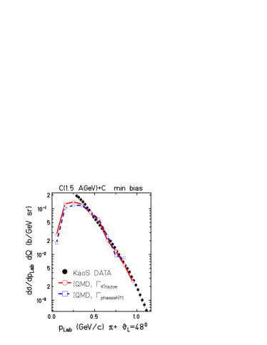
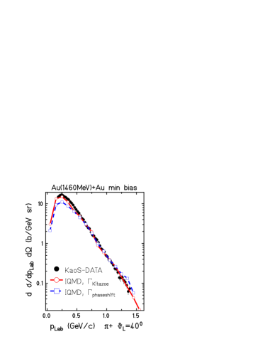
Figure 10: Comparison of IQMD pion spectra using different delta lifetimes with KaoS data for C+C (left) and Au+Au (right) at 1.5 AGeV incident energy.

We see that at these energies the data support rather the Kitazoe parametrization. However, at lower incident energies the yields are better described by the phase-shift parametrization. Furthermore it should be noted that both parametrizations agree in the high energy part. We see that also the dynamics of the pions seems to be described sufficiently.

III Production of $K^{+}$

III.1 The elementary production

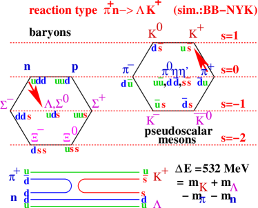
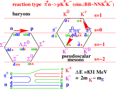
Figure 11: Description of the major elementary channels of $K+$ production in a $\pi^{+}n$ collision

The elementary production of $K^{+}$ is governed by the conservation of strangeness. The initial net strangeness is zero, thus strange quarks can only be produced together with strange anti-quarks. In the multiplett scheme shown in fig. 11 this means that the sum of the red arrows should be zero. The most economic way to do this is to create an $s$-quark which remains in a baryon (and thus transforms the nucleon into a hyperon) together with a $\bar{s}$-quark which joins the kaon. An example of such a process is given on the l.h.s. of fig. 11, where the reaction $\pi n\to\Lambda K^{+}$ is described. In this reaction a $d\bar{d}$-pair annihilates to form a $s\bar{s}$ pair. This reaction only needs an energy of 532 MeV available in the centre-of-mass while a reaction of producing a $K^{+}K^{-}$ pair (r.h.s.) and leaving the nucleon a nucleon needs much more energy. When regarding the quark diagrams on bottom of fig. 11 we see that the latter process creates an additional $u\bar{u}$ pair and should thus be suppressed by OZI rules.

The same argument holds when regarding baryon-baryon reactions. The channel $B_{1}B_{2}\to B_{3}YK^{+}$ has lower thresholds than the channel $B_{1}B_{2}\to B_{3}B_{4}K^{+}K^{-}$. Here $B$ may be a nucleon $N$ or a delta $\Delta$ and $Y$ may be a $\Lambda$ or a $\Sigma$ and we end up to a large amount of reactions which need to be described. The list of all $K^{+}$ production reactions parametrized in IQMD is shown in table 2.

$NN\to N\Lambda K^{+}$	$NN\to N\Sigma K^{+}$	$NN\to\Delta\Lambda K^{+}$	$NN\to\Delta\Sigma K^{+}$
$N\Delta\to N\Lambda K^{+}$	$N\Delta\to N\Sigma K^{+}$	$N\Delta\to\Delta\Lambda K^{+}$	$N\Delta\to\Delta\Sigma K^{+}$
$\Delta\Delta\to N\Lambda K^{+}$	$\Delta\Delta\to N\Sigma K^{+}$	$\Delta\Delta\to\Delta\Lambda K^{+}$	$\Delta\Delta\to\Delta\Sigma K^{+}$
$\pi N\to\Lambda K^{+}$	$\pi N\to\Sigma K^{+}$	$\pi\Delta\to\Lambda K^{+}$	$\pi\Delta\to\Sigma K^{+}$
$NN\to NNK^{+}K^{-}$	$N\Delta\to NNK^{+}K^{-}$	$N\Delta\to N\Delta K^{+}K^{-}$	$\Delta\Delta\to NNK^{+}K^{-}$
$\Delta\Delta\to\Delta\Delta K^{+}K^{-}$	$\pi N\to NK^{+}K^{-}$	$\pi\Delta\to NK^{+}K^{-}$

Table 2: List of the $K^{+}$ producing reactions parametrized in IQMD

In these channels different isospin combinations for $N,\Delta,\pi$ are possible which yields a further subdivision of these channels. Note that we only use the $\Delta(1232)$ which is the dominant resonance channel in this energy domain.

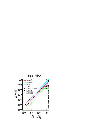
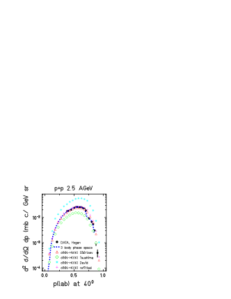
Figure 12: Parametrizations of the $pp\to p\Lambda K^{+}$ channels (left) and comparison of IQMD with pp-data

Most of these channels are not accessible experimentally. Even for the channel $NN\to N\Lambda K^{+}$ only the isospin combination $pp\to p\Lambda K^{+}$ is known by experiment. At energies close to the threshold still a lot of uncertainties are remaining. Fig. 12 shows on the l.h.s. several parametrizations of this channel used by our simulations. Our standard parametrization is that of Sibirtsev et al. sibirtsev (red full line with triangles) fitted to data cited in his publications. Other possibilities are the parametrization by Tsushima et al tsu (green dash-dotted line with diamonds) and a parametrization of David et al david (cyan line with stars) fitting recent COSY data cosy98 . This fit has later on be modified including data points at higher energies (magenta line with crosses) and reads:

$$\sigma(pp\to p\Lambda K^{+})=191\mu b\cdot\left(\sqrt{s}-\sqrt{s_{\rm thres}}\right)^{1.43}$$ (18)

This parametrization is of course only valid for energies not higher than about 3 GeV, which is however a limit of IQMD.

Other channels have to be extrapolated by isospin-considerations. When calculating in the One Boson Exchange model the choice of the exchange particle (pion or kaon) changes the factor to extrapolate from pp to pn from 1 to $5/2$. In IQMD the latter factor of 5/2 is used which causes an isospin averaged cross section of

$$\sigma(NN\to NYK^{+})=\frac{1}{4}\bigl{(}\sigma_{pp}+2\sigma_{pn}+\sigma_{nn}\bigr{)}=\frac{1+5+0}{4}\sigma_{pp}=\frac{3}{2}\sigma(pp\to NYK^{+})$$ (19)

For the channels including $\Delta$ no knowledge from experiment exists. Here exists some freedom in assuming the cross sections which raises uncertainties in the interpretation of heavy ion data. We will come to this point later on. For our parametrization results of calculations performed by Sibirtsev sibirtsev are used for the channel $\sigma(NN\to N\Lambda K^{+})$ while for all other channels the parametrizations of Tsushima et al. tsu are used.

The right hand side of fig.12 compares results of experimental pp-data of Hogan et al hogan (black bullets) with IQMD calculations (red triangles) using the Sibirtsev and Tsushima cross sections. The agreement shows that in the known sector of cross sections our parametrizations work well. A replacement of the $\sigma(NN\to N\Lambda K^{+})$ cross section by the corresponding cross section of Tsushima tsu (green diamonds) would yield a too small yield which explains the choice taken for IQMD. The parametrization of David david (cyan stars) yields too much kaons since its cross section is too high at high energies. The refitted parametrization (magenta crosses, see eq. 18) shows again a spectrum quite comparable to that using the Sibirtsev parametrization.

Another important point to be discussed in this figure is the dynamics of the collision itself. Since there are three particles in the outgoing channel, there is some freedom in determining the dynamics of the particles within the constraints of the conservation laws. One possibility is to create an intermediate resonance which decays into two particles.

$$NN\to RN\qquad R\to YK^{+}\qquad R=N^{*}(1650),N^{*}(1710)\mbox{etc}$$ (20)

This procedure is e.g. done in UrQMD urqmd . In IQMD the two colliding particles form one intermediate resonant two particle state which decays directly into three particles by a three-body decay.

$$NN\to R\qquad R\to NYK^{+}\qquad M(R)=\sqrt{s}$$ (21)

The experimental data at these energies support the dynamics of a three-body phase space model (blue dotted line) as it is implemented in IQMD. However, at higher energies the phase space model describes the data less well.

III.2 Subthreshold production

Subthreshold production is the production of particles at an incident energy at which a production in a free p+p collision is no more permitted due to energy-momentum conservation. For the production of kaons the production threshold is constrained by the conservation of strangeness. The lowest threshold for a reaction producing a kaon is given by the channel $p+p\to p+\Lambda+K^{+}$

$$\sqrt{s}=\sqrt{\sum P_{\mu}P^{\mu}}\geq m_{p}+m_{\Lambda}+m_{K^{+}}=2.55{\rm GeV}\qquad P=p_{1}+p_{2}$$ (22)

where $p_{1}$ and $p_{2}$ are the four-momenta of the colliding particles. This implies a minimum incident energy of around 1.58 AGeV of the proton projectile on the proton target. In heavy ion collisions kaons can also be produced at lower incident energies. There are majorly two effects which allow this subthreshold production

1. Due to the Fermi momentum of the nucleons in projectile and target two colliding particles may have a higher energy than given by the incident energy. This may allow to reduce the threshold incident energy up to around 1 AGeV.

2. Due to rescattering of the nucleons some nucleons may accumulate energy such that finally sufficient energy is given for the production of kaons. Resonances may serve as energy storage since they transform kinetic energies into mass. Two nucleons of projectile and target may collide and create a delta which due to its higher mass will be quite slow. Another fast projectile nucleon may collide with this delta and produce a kaon. Or, if another delta is formed by two other nucleons of projectile and target and create a delta and these two delta collide, there is no much need for high additional energy. The sum of the two masses (the peak of the delta mass distribution is at around 1.232 GeV) is already nearby the threshold. With this mechanism one may create kaons even at a few hundred MeV of incident energy. However the probability will be quite small and depend strongly on the system size.

After fixing the cross section parametrizations to pp-data we now can use our models for the simulation of heavy ion collisions. Let us first start with some analysis of p+A.

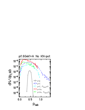
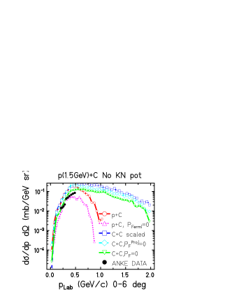
Figure 13: Comparison of p+p, p+C and p+Au momentum spectra at 1.6 GeV (left) and of p+C and C+C spectra at 1.5 AGeV (right)

The left hand side of fig. 13 shows the lab momentum distribution of p+A collisions at 1.6 GeV incident energy, i.e. slightly above the threshold. In a p+p case (black dotted line) there is a quite narrow distribution. Only little energy is available to the kaon, which is produced in the centre-of-mass of the reaction. Thus it carries only a momentum slightly different to the centre-of-mass momentum. In the p+C collision (blue dashed line) there is a much wider distribution. This is only in part due to the Fermi momentum in the carbon target where the projectile may collide with a particle with a Fermi momentum in the opposite direction of its momentum and thus enhance the available energy of the kaon. This can be seen when comparing the p+p curve (black dotted line) and the p+C curve (with Fermi momentum, blue dashed line) with a calculation without Fermi momentum (p+C, $\rm P_{Fermi}=0$, cyan curve with diamonds). The major part of the difference between p+p and p+C stems from the opening of additional channels due to multi-step processes: $N_{1}N_{2}\to N\Delta,\quad N_{3}\Delta\to NYK$ ($N\Delta$ channel) and $N_{1}N_{2}\to N\Delta,\quad\Delta\to N\pi\quad\pi N_{3}\to YK$ ($N\pi$ channel) which in the case of p+C contribute to more than 80 % to the total kaon number. A further rise is gained by the Fermi momentum, which allow for enhancing the available energy by selecting a partner which opposite Fermi momentum. Since the cross section increases strongly nearby the threshold (see fig. 12) it allows for a strong enhancement of the kaon production especially for the $NN$ channel which regains the dominance in a p+C collision if the Fermi momentum is on. All effects contribute to the effect that the total production probability is strongly enhanced with respect to the p+p case. Finally if the first collision takes the elastic channel (which at high energies is strongly forward-backward peaked) there is a further chance in producing a kaon in another collision of the projectile nucleon with a target nucleon. These effects explain the huge increase of the kaon multiplicity when going from p+p to p+C. When going from p+C (blue dashed line) to p+Au (red full line) there is an additional increase at low laboratory momenta. This is probably due to second chance effects. If the projectile looses only little energy in its first collision(s) it may still produce a kaon in a secondary collision if the Fermi momentum of the target nucleon supports this. For the Au case there is much more chance to find such a particle. The kaon is no more produced in the p+p centre-of-mass but in the centre-of-mass of the slowed down projectile with a target nucleon. This explains the shift toward lower lab momenta which can be seen as well in calculations with (red full line) and without (green dash-dotted line) Fermi momentum.

The right hand side of fig. 13 compares calculations at 1.5 AGeV incoming energy, i.e. already below the threshold. A p+p collision cannot produce a kaon any more. The forward angle laboratory momentum distribution of IQMD events (red full line) is compared to data of the COSY-ANKE collaboration anke . We see a qualitative agreement which supports the existence of the effects stated above. A p+C calculation without Fermi momentum (magenta dotted line with upward triangles) shows again a strongly reduced kaon yield which again demonstrates the importance of multi-step processes. Furthermore a minimum bias reaction of C+C (blue dashed line) has been scaled by the different reaction cross sections and the average number of participant projectile nucleons. This allows to compare a C+C collision to a $A_{part}\times$p+C collision, an idea which corresponds to the Glauber-model. We see a similar behavior at low lab momenta but a much wider range of available laboratory momenta. This is less due to the additional Fermi momentum in the projectile but majorly there is now the possibility of accumulating the energy of several collisions of projectile nucleons and target nucleons (for instance in forming two deltas which collide). We see that calculations where the Fermi momentum of the carbon has been removed for the projectile only (cyan curve with diamonds) or for both nuclei (green curve with downward triangles) show a similar enhancement at high energies. This already demonstrates the importance of the full nucleon dynamics, multi-collision effects, resonance production and so on. We will therefore address this subject more in detail.

III.3 The major production channels

At first, we want to address the question, which channel is important for heavy ion collisions. Fig. 14 shows the kaon yield in a collision of Au+Au at 1.5 AGeV incident energy as a function of the impact parameter(black dotted line). We see a strong centrality dependence, where the production of kaons is strongest supported in central collisions. A decomposition of the kaon yield into the producing channels shows that the $NN$ channel (blue dashed line) only contributes quite weakly while the addition of the $N\Delta$ channel already describes the major part of the yield.

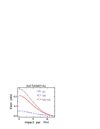
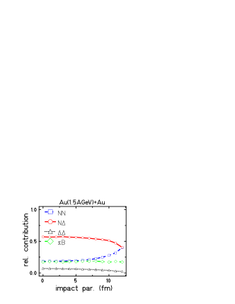
Figure 14: The absolute kaon yield (left) and the relative contribution (right) of different production channels as function of the impact parameter in a Au+Au collision at 1.5 AGeV incident energy.

The right hand side of fig. 14 shows the relative contribution of the different channels implying nucleon-nucleon collisions ($NN$, blue dashed line), delta-nucleon collisions ($N\Delta$, red full line), delta-delta collisions ($\Delta\Delta$, black dotted line) and pion-baryon collisions ($\pi B$, green dash-dotted line). The $N\Delta$ channel dominates the production over a large impact parameter range. Only in very peripheral collisions the rather weak $NN$ channel runs up to become as important as the $N\Delta$ channel.

Fig. 15 shows the relative contribution of the different channels ($NN$ - blue dashed line, $N\Delta$ - red dashed line, $\Delta\Delta$ - black dotted line, $\pi B$ - green dash-dotted line) as function of energy and system size.. At the left hand side the excitation function of Au+Au is shown, while on the left hand side the dependence on the system size for b=0 collisions at 1.5 AGeV incident energy is studied.

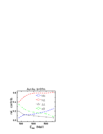
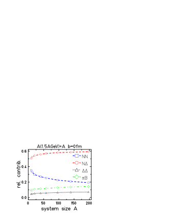
Figure 15: Contribution of different production channels to the kaon yield as function of incident energy (left) and system size (right)

We see the contribution of $NN$ is rather small especially at low energies. Note that only the highest energy point of 1.8 AGeV has enough energy to produce a kaon directly. The same reaction done with p+p would not produce any kaon at incident energies below 1.6 GeV. In order to get the energies necessary for a kaon production, the system has to cumulate energy. This might be done by the creation of resonances (like the $\Delta$) or pions. Therefore, the $N\Delta$ channel has the strongest contribution. The $\Delta\Delta$ channel gains even more energy but the possibility that two deltas collide is rather small. But if the system goes down to very low incident energies, the need for energy cumulation is that high that even these rare channels start to play an important role. The same is true for the $\pi B$ channel where a high energy pion has to find a $\Delta$ or a high energy nucleon for producing a kaon.

Let us now look at the system size dependence (r.h.s.) of the channel contributions. We are at rather high energies (1.5 AGeV, slightly below the threshold) where already the Fermi momentum of the nucleons may help the nucleons to produce kaons in first collisions. Therefore, the contribution of the rare combinations $\Delta\Delta$ (black dotted line) and $\pi B$ (green dash-dotted line) is rather small. The $N\Delta$ (red dashed line) channel dominates, but the $NN$ channel contributes quite well especially for small systems. For these systems we have a larger contribution of the surfaces, where we could expect first $NN$ collisions. This effect is in agreement with the impact parameter dependence seen in fig. 14 where the $NN$ channel becomes important in very peripheral collisions where only the surfaces of the nuclei touch.

III.4 The collision history

Next we want to discuss the aspect of cumulating energy in analyzing the collision number of the parents. Fig. 16 shows on the left hand side the relative fraction of nucleons as a function of the number of collisions the particles had during the reaction. We see that for a light C+C system (blue dashed line) the maximum is reached for about 2 collisions while for the heavy Au+Au system (red full line) most of the particles had about 6 collisions.

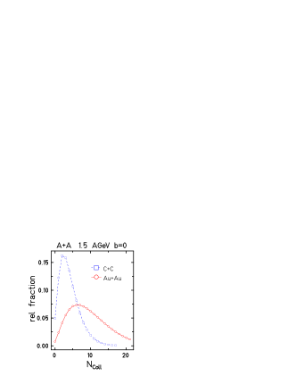
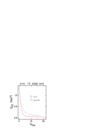
Figure 16: Fraction of nucleons having a given collision number (left) and sphericity $Q_{ZZ}$ as function of the collision number (right) for Au+Au and C+C

The right hand side of fig. 16 shows the sphericity value $Q_{ZZ}$ as a function of the collision number. $Q_{ZZ}$ is defined by

$$Q_{ZZ}=3p_{Z}^{2}-p^{2}=2p_{Z}^{2}-p_{T}^{2}=2p_{Z}^{2}-p_{X}^{2}-p_{Y}^{2}$$ (23)

$Q_{ZZ}>0$ defines a prolate momentum ellipsoid and $Q_{ZZ}<0$ an oblate one. An isotropic distribution yields $Q_{ZZ}=0$. We see that the system approaches isotropy with increasing collision number and that at least 3-6 collisions are necessary to come nearby equilibration.

We now analyze for each kaon the sum of the collisions each partner had up to the production of the kaon. If the kaon is produced in one of the first collisions, the sum of the collision numbers of the parents should be 2 (first collision for each partner). If the kaon is produced in an ‘equilibrated medium’ than this number should be much higher. As each particle needs more than 3 collisions for equilibrating, therefore this number should be at least 6 or higher.

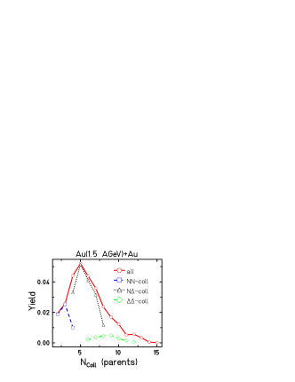
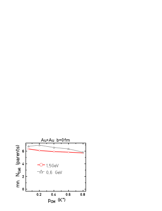
Figure 17: Distribution of the number of collisions the parents had when producing of the kaon selected according to different production channels (left) and to the momentum of the kaon (right)

The left hand side of fig. 17 shows the distribution of the number of collisions the parents had when producing of the kaon selected according to different production channels. In the $NN$-channel (blue dashed line) the parents did undergo only a few collisions. The very first collisions ($N_{Coll}=2$) contribute strongly and the other contributions are majorly the first collision of an incoming particle with the stopped matter in the centre. This is easy to understand since the incident energy is weakly below the threshold energy. Thus, already the Fermi momentum of the particles is sufficient to overcome the threshold.

In the $N\Delta$-channel (black dotted line) the maximum of the distribution is at $N_{Coll}=5$, i.e. for collisions where at least one particle is nearby equilibration. In the $\Delta\Delta$-channel (green dash-dotted line) the numbers are even higher.

The mean value of the distribution is around 6 as we can easily see on the right hand side of fig. 17, where we describe the mean value of the sum of the parent collision numbers as function of the centre-of-mass momentum of the outcoming kaon. The function is flat, which means the the production of higher energy kaons does not need more collisions of the parents. With about 6 collisions at least one partner has become equilibrated and more collisions do not equilibrate more. The only questions is now to find a particle in the tail of the energy spectrum which has sufficient energy for producing a kaon. This finding is supported by the observation that the number of parental collisions does not change very much with the incident energy. A reaction far below threshold (0.6 GeV,black dotted line) gives only slightly higher numbers than a reaction nearby the threshold (1.5 GeV, red full line). Moreover there is no significant system size dependence. A C+C collision yields at 1.5 GeV about the same values than a Ni+Ni or Au+Au collision.

III.5 Production time and density

Let us now look at the question when the kaons are produced. The left hand side of fig. 18 shows the time profile of the produced kaons selected according to their production channels.

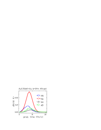
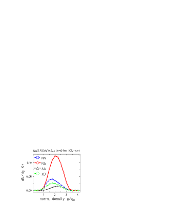
Figure 18: Time and density profile of kaon production

We see that the $NN$ channel (blue dashed line) starts first, shows a maximum at about 6 fm/c and falls down rapidly afterward. This corresponds to the assumption that this channel is majorly fed by the first collisions at the beginning of the reaction. The $N\Delta$ channel (red full line) starts a little bit later to show a maximum at about 8 fm/c (which corresponds to the time of maximum compression. The $\Delta\Delta$ channel (black dotted line) starts even later. This corresponds to the observation of the left hand side of fig. 17 that the $\Delta\Delta$-channel shows the biggest number of parental collisions for the production. This creation of highly stopped matter, of course, needs some time, before this channel becomes active. The $\pi B$ channel (green dash-dotted line) also starts late. Here we have to keep in mind that in the beginning the pions are rapidly reabsorbed into deltas and come out quite late. Therefore, the pion number increases slowly which allows the pion channel only to start later.

The right hand side of fig. 18 shows the density profile of the different channels. The early $NN$ channel (blue dashed line) reaches quite moderate densities which corresponds to the previous picture that this channel is happening early in the non-equilibrated matter which is still in compression. The $N\Delta$ channel (red full line) reaches higher densities. The distribution peaks at about two times normal nuclear matter. The maximum of the distribution of the $\Delta\Delta$ channel (black dotted line) is even a little bit higher. This is in alignment to the high number of parental collisions (which can be reached best in the high density zone) and to a production time in the range of highest compression. The $\pi B$ channel (green dash-dotted line) finally prefers less high densities. In the high density zone pions are rapidly absorbed to deltas and thus more pions are available at lower densities.

III.6 Where are the kaons produced?

Let us now address the question, where the kaons are produced. Fig. 19 shows the radial density-profile of the kaon production with respect to the centre of the reaction.

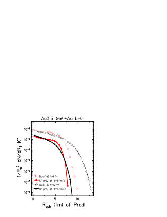
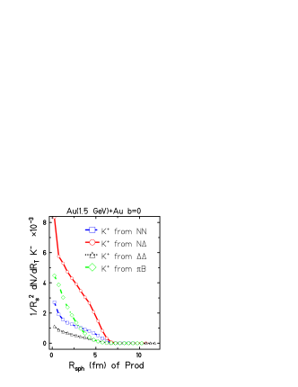
Figure 19: Radial distribution of kaon production selected according to production time and to channel decomposition

We see on the left hand side a comparison of the nuclear radial distribution (dotted curves with open symbols) at $t=8$ fm/c (max. compression, red circles) and $t=12$ fm/c (end of kaon production, black triangles) with the distribution of the production points of kaons produced at the same time windows (full curves with full symbols). The nuclear distributions are broader than the kaon production distributions and the differences become stronger at the surfaces. From this we can conclude that the kaons are really produced in the central part of the reactions.

The right hand side of fig. 19 shows the time integrated radial distribution of the kaon production on a linear scale selected according to different channels. We see that for all channels there is a peaking of the distribution at $R=0$, i.e. in the centre of the reaction.

III.7 Is there sensitivity to the nuclear eos?

We can conclude from the previous analysis that the kaon production at the discussed energies is strongly related to a high compressed region where energy may be cumulated in multi-step processes. We may therefore rise the question whether the kaon production might be a good signal for determining the nuclear equation of state.

The nuclear equation of state describes the property of nuclear matter to be compressed. A hard equation of state (having a high compressibility) gives a strong repulsion to the compression. More compressional energy is needed to compress the system to a given density. A soft equation of state (with less compressibility) resists less to the external compression and allows for higher densities for a given compressional energy. In a heavy ion collision thus a higher maximum compression can be reached when employing a soft equation of state (red full line) than when using a hard one (blue dashed line), as it can be seen on the left hand side of fig. 20 where we compare the time evolution of the central density for both equations of state.

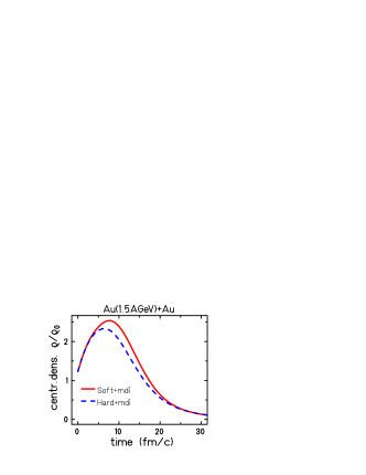
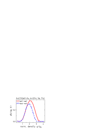
Figure 20: Time evolution of the central density in a calculation with hard and soft eos (left) and density distribution of the kaon production within a calculation without potentials (right)

A higher density means a smaller mean free path and thus a better possibility to gain the energy necessary for kaon production via multi-step processes. Therefore, the kaon production should be enhanced for a soft eos aik . The right hand side of fig. 20 shows that indeed the number of kaons is enhanced when a soft equation of state is employed (red full line) and that the additional kaons just come from the regions with higher densities.

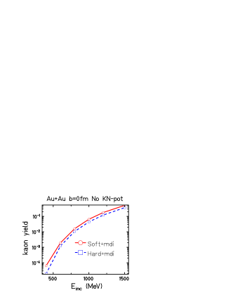
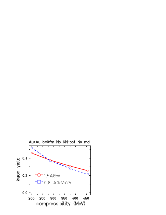
Figure 21: Excitation function of kaon yield for a calculation without KN-potentials (left) and kaon yield as function of compressibility

Therefore, the kaon production shows a sensitivity to the equation of state as we can see it on the left hand side of fig. 21  where we compare the excitation function of kaon production with a hard (blue dashed line) and a soft (red full line) eos. The right hand side  shows the dependence of the kaon production on the compressibility of the equation of state. A softer eos (small compressibility) yields a higher kaon number than a harder one. This effect is even stronger when we reduce the incident energy from 1.5 AGeV (red full line) to 0.8 AGeV (blue dashed line). At lower energies there is more sensitivity to the available density since we are more dependent on the production of kaons in multi-step processes.

However, the argument is not as simple as shown. We will first have to attack some questions on the nuclear medium and uncertainties of the cross section before we can revisit the question of the nuclear equation of state.

IV Kaons in the medium

When the kaons are in the nuclear medium of a heavy ion collision several effects will have to be taken into account.

1. The kaons may rescatter. This may influence dynamical observables as we will see later on.

2. The repulsive optical potential of the $K^{+}N$ interaction may deviate the trajectories of the kaons.

3. The repulsive optical potential of the $K^{+}N$ interaction may penalize the production of kaons and change the threshold effectively since the kaons are produced at higher effective masses.

IV.1 Rescattering of kaons

Kaons rescatter with nucleons with a cross section of about 13 mb at lower relative momenta. Since the nuclear matter is highly compressed in the region of kaon production there is a high chance of kaon rescattering.

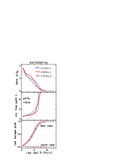
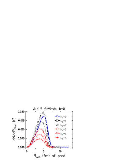
Figure 22: Radial densities of nucleons and the resulting escape probabilities of $K^{+}$ (left) and the radial production profile of $K^{+}$ selected according to the number of collisions (right)

The left hand side of fig. 22 shows on top the radial density distribution of the nucleons at time steps of $t=4$ fm/c (blue dashed line), $t=8$ fm/c (red full line) and $t=12$ fm/c (black dotted line). The times of 4 and 12 fm/c correspond to the time window when most of the kaons are produced, while 8 fm/c corresponds to the maximum compression and the maximum kaon production. From this density we can derive by assuming a cross section of 13 mb a mean free path as depicted in the mid of the left hand side of fig. 22. An integration over the mean free path finally gives an escape probability of leaving the system without a collision (bottom). This probability of course depends on the exact way the kaon takes. We therefore indicate the best case (a direct radial escape) and a worst case (an escape in the opposite direction). We should note that most of the kaons are produced in a three body decay and therefore the kaons take a high momentum with an isotropic distribution in the centre-of-mass frame of the collision. The collision frame itself has a rather small velocity for maximum kinematic use of the energy of the colliding particles. Therefore, the velocity of the sources plays no important role and the kaon will choose its direction randomly. The right hand side of fig. 22 shows the radial distribution of the kaons selected according to their collision number. Note that we plot the radial distribution while in fig. 19 the radial density was plotted, which takes into account the volumes of the radial cells. We see, that at the production radii the probability of escape is rather reduced. We see further that the multicolliders really stem from rather small radii.

Therefore, we may assume that the kaons really stemming from highest densities have the highest chance to collide.

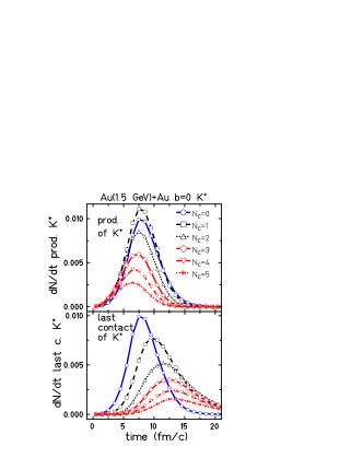
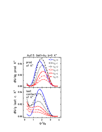
Figure 23: Time and density profiles for production and last contact selected according to collision number

Fig. 23 shows again the profiles of production times (left) and density (right) selected according to the number of collisions. Multicolliding kaons (red curves) are produced very early and at very high density but their last collision contact is quite late and happened at rather low density. Therefore, the idea to look for the dynamics of kaons in order to learn something on the high density region will be constrained by the effects of rescattering.

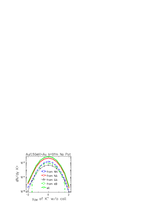
Figure 24: Rapidity distribution of $K^{+}$ selected according to their collision number (left) and of $K^{+}$ without collisions selected according to their production channel (right)

The effect of rescattering to dynamical observables is illustrated in fig. 24 where we show the rapidity distribution of kaons selected according to their collision numbers. We see on the left hand side that kaons without collisions (full blue line) show a smaller distribution than kaons which did undergo collisions. Therefore the rapidity distribution of kaons is broader when rescattering is active. For comparison we see on the right hand side of fig. 24 the comparison of the effect of the incident channels on the rapidity distribution for particles without collisions. Kaons stemming from high-density $\Delta\Delta$ collisions (black dotted line) show a broader distribution than kaons stemming from $NN$ (blue dashed line) but this effect will be overruled by the effect of rescattering.

Further discussion of the effects of rescattering on dynamical observables can be found later on.

IV.2 Influence of the optical potential

The optical potential of the kaon in the nuclear medium is repulsive for $K^{+}$ and enhances its effective energy in the medium. Thus, the production of a kaon in the medium needs more energy than in the free case and enhances the threshold of its production. Since we are at energies below the elementary threshold and since we already need to cumulate energy for getting a kaon, this up-shift of the threshold yields a strong reduction of the kaon yield.

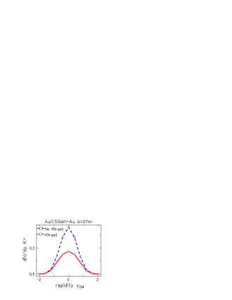
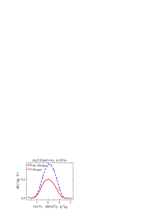
Figure 25: Rapidity distribution and density profile of kaon production with and without kaon potential.

Fig. 25 shows on the left hand side the effect of the optical potential on the rapidity distribution of kaons at Au(1.5AGeV)+Au b=0. A calculation with optical potential (KN-pot, red full line) yields much less kaons than a calculation without optical potential (blue dashed line). Especially at mid-rapidity the discrepancy is most prominent. Here the kaons with least energy can be found. They are produced by collisions slightly above the production threshold, thus only few energy is available for the kinematics. Here a shift of the threshold inhibits their production. Kaons with high absolute values of the rapidity have rather high energies. In their production the shift of the threshold reduced the remaining energy for the kinematics. However, the repulsive potential gives back this energy when the kaon will leave the medium in the late expansion phase. We will see later on similar effects for the spectra.

The right hand side of fig. 25 shows the density profile of the kaon production in both calculations. We see that the penalty of the potential acts especially at high densities since here the shifts of the threshold are the strongest.

This penalty also effects the excitation function of the kaons as we can see from the left hand side of fig. 26. At low incident energies the production of kaons via multi-step processes is more important than close to the threshold. Remember that the effect of the eos was also stronger at lower energies due to the same argument. Therefore, the penalization of reactions at high densities shows stronger effects which causes a strong influence of the calculation with (red full line) and without (blue dashed line) an optical potential The effect of the energy loss can also be seen when comparing the calculation with optical potential (and full Fermi momentum, red full line) with a calculation with optical potential where the Fermi momentum has been suppressed (black dotted line). The lack of Fermi momentum gives an additional lack of energy which shows strongest effects at low energies where the multi-step processes very important and where a multiple lack of energy reduces the yield drastically.

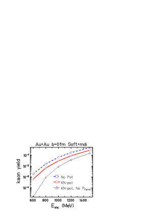
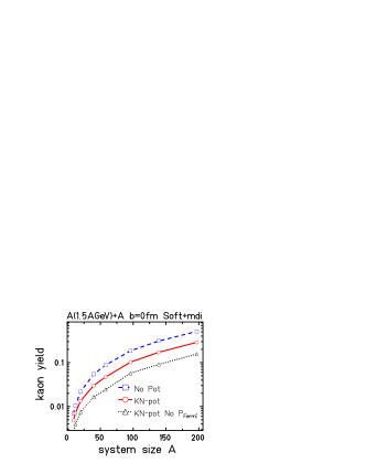
Figure 26: Excitation function (left) and system size dependence (right) of the kaon yield with and without KN-potential and with KN-potential but no Fermi momentum.

The system size dependence of kaon production shown in right hand side of fig. 26 shows only weak effects for small systems but strong effects for large systems. In small systems the compression is weaker and less high densities are reached. Therefore, the penalty of the potential is weaker. Also the effect of the missing Fermi momentum is smaller.

This interplay of density and penalty can also be demonstrated nicely when analyzing the effects of the scalar and vector part of the optical potential as it is shown in fig. 27.

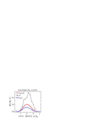
Figure 27: Rapidity distribution and density profile of kaon production and the contribution of scalar and vector part.

The scalar potential (black dotted line) is attractive (see fig. 4). It enhances the kaon yield especially at mid-rapidity. Since the penalty at high densities is changed into a gain, it strongly enhances the kaon yield. The gain is stemming dominantly from the high densities. The vector potential is very repulsive. A calculation using only the vector potential (blue dashed line) reduces the kaon number particularly at mid-rapidity and reduces the production especially at high densities.

The effect of the strength of the optical potential can finally be seen in fig. 28 where we compare different parametrizations of the optical potential. A parametrization with less strength (half pot, green dash-dotted line, see fig. 3) yields higher kaon numbers than our standard optical potential (Schaffner RMF, red full line), a parametrization with a comparable strength (NJL, T=150, black dotted line,see fig. 5) a comparable kaon distribution and a calculation with a higher strength of the potential (NJL, T=0, blue dashed line,see fig. 5) a smaller kaon number.

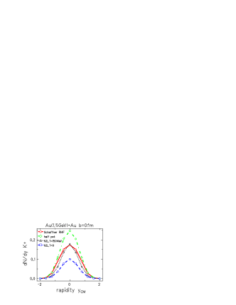
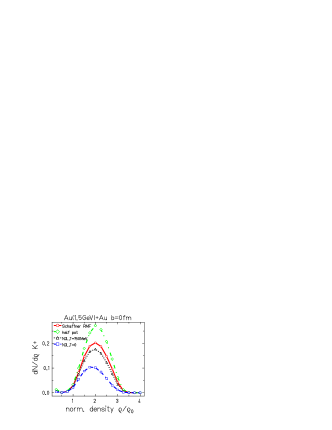
Figure 28: Rapidity distribution and density profile of kaon production for different parametrizations of the optical potential.

Again, the effect is most significant at mid-rapidity and effects mostly the kaons stemming from high densities. Different parametrizations of the optical potential may thus yield different kaon yields.

The effect of the optical potential on spectra, temperatures and angular distributions will be discussed later.

V Can we derive the potential from kaon yields?

As we have seen the optical potential shifts the up the production threshold and thus reduces the kaon yield. A strong repulsive potential yields therefore a strong reduction of the kaon yields while a weak repulsion yields a weak reduction of the yield. We will now address the question whether this effect might be used to determine the kaon optical potential.

V.1 Comparison to p+A

Let us start with p+A data which have already been shown to be quite sensitive to the kaon production mechanisms.

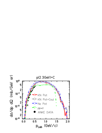
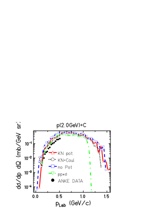
Figure 29: Comparison of p+C data at 2.3 and 2.0 GeV

In fig. 29 a comparison of COSY-ANKE p+C data (bullets) anke and IQMD calculations with (red full line with triangles) and without KN potential (blue dashed line with squares) for energies of 2.3 (left) and 2.0 GeV (right) is shown. We see that the calculation without potential yields slightly higher results than the calculations with potential. The additional inclusion of Coulomb forces (black dotted line with circles ) does not yield a significant change since the target is quite light. The data support rather the calculations with potential. A comparison of p+C with a scaled p+p reactions (green dash-dotted line) shows again the importance of the Fermi momentum to describe the high momenta. Unfortunately no experimental data are available at these high momentum values.

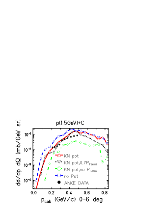
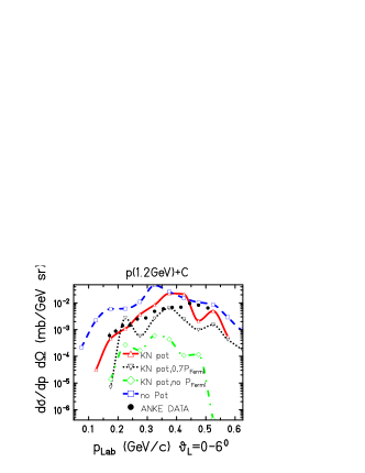
Figure 30: Comparison of p+C data at 1.5 and 1.2 GeV

However, the difference between calculations with and without potentials is quite small. This is due to the high incident energy. The higher the energy above the threshold the less important becomes the penalty of the optical potential caused by the threshold shift. Therefore fig. 30 presents calculations below the threshold. Here the importance of the potential becomes stronger when going further down in energy as we can see when comparing p+C at 1.5 GeV (left) and 1.2 GeV (right). The data seem to comply better with the calculation with an optical potential (red full line) than with a calculation without potential (blue dashed line). However, the result far below subthreshold depend strongly on the description of the energy available in the nucleus. If we use a calculation with potential and reduce the Fermi momentum from its full value (red full line) to only 70 % (black dotted line) we also reduce the kaon production significantly. A complete suppression of the Fermi momentum (green dash-dotted line) shifts the results visibly beyond the experimental data.

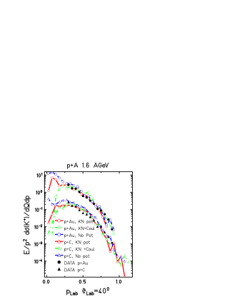
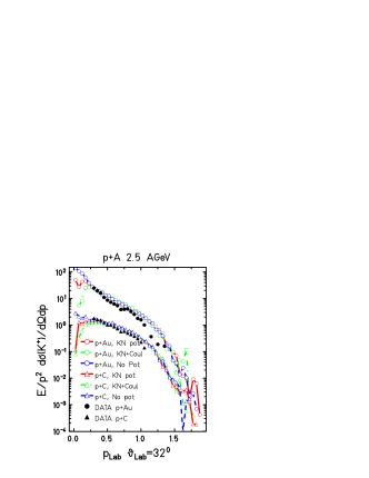
Figure 31: Comparison of p+C and p+Au KaoS data at 1.6 and 2.5 GeV

The ANKE data are measured at very small laboratory angles. As an effect, comparison these spectra might be influenced by rescattering. A rescattered kaon may easily leave that small detector angle. Therefore it is interesting to compare kaons also at other laboratory angles. In fig. 31 we see recent spectra of the KaoS collaboration scheinast taken at laboratory angles of $40^{0}$ (1.6 GeV, left) and $32^{0}$ (2.5 GeV, right). We find a visible influence of the optical potential. However, a conclusion on the potential is quite difficult. The inclusion of Coulomb forces (green dash-dotted line) only changes the spectra at very low momenta where no experimental data are available. We see that the Coulomb forces show a stronger effect for the heavy Au system than for the light C system due to the larger charge of the nucleus.

V.2 Influence of rescattering in p+A

Let us now analyze the influence of the rescattering on the kaon spectra. As indicated rescattering may change the direction of the outcoming kaon and also change its energy. Fig. 32 shows how the rescattering effects the spectra. The full lines show spectra with normal rescattering, the dashed lines calculations without rescattering and the dotted lines calculations with a doubled value of the rescattering cross section.

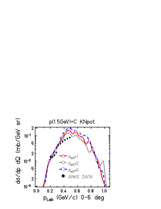
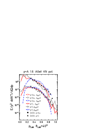
Figure 32: Comparison of p+A spectra with normal rescattering, disabled rescattering and rescattering with the double cross section.

We see for the spectra at small angles (left hand side) an enhancement of the absolute yield when suppressing rescattering and a diminution of the yield when enhancing the rescattering. A rescattered kaon leaves that detector angle. For the spectra at higher angles (right hand side) the low momentum part increases with rescattering and decreases when turning off the rescattering. The effect is stronger for a heavy system (p+Au) which allows for more rescattering partners than for a light system.

V.3 Influence of delta lifetime and of the nucleon-nucleon cross section on the kaon production in p+A

Let us now shortly discuss the effect of the delta lifetime on the spectra in p+A. Since at low incident energies the $NN$ channel still plays an important role and no high density region is built up there should be no strong influence of the lifetime of the delta on the spectra. This can be seen in fig. 33.

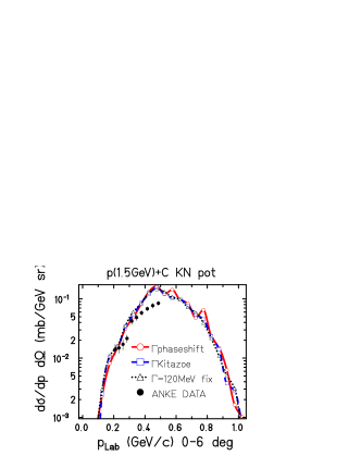
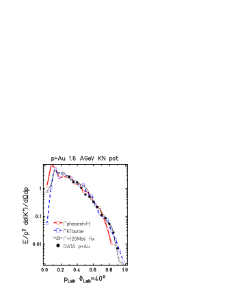
Figure 33: Comparison of p+A spectra with different parametrizations of the delta lifetime

However this delta lifetime may play a role when discussing A+A. We will soon come back to this point. We should also note that a strong reduction of the Fermi momentum enhances the contribution of the $N\Delta$ and $N\pi$ channels and may enhance the significance of the delta lifetime for this case.

The nucleon-nucleon cross section influences the dynamics of the nucleons and the production of resonances. However, like in the discussion of the delta lifetime there is no big effect on the p+A results if we use an unchanged production cross section of the kaons. This can be seen in fig. 34.

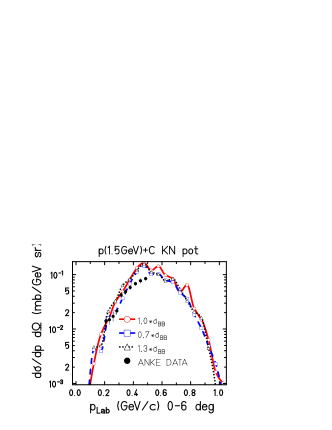
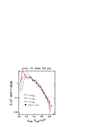
Figure 34: Comparison of p+A spectra with different factors to the nucleon cross section.

V.4 Uncertainties of unknown production cross sections

As is was shown in fig. 15 the major contribution to kaon production is the $N\Delta$ channel. Unfortunately, this channel is not accessible experimentally. Thus, cross section parametrizations of this channel have some relative freedom relying on different assumptions.

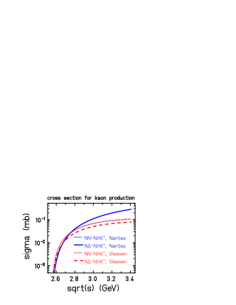
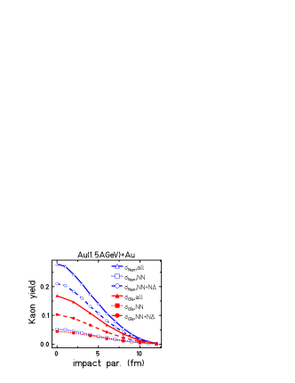
Figure 35: Different parametrizations of the $N\Delta\to N\Lambda K$ cross sections and its influence to the kaon yield.

As an example the HSD-group in Giessen cassing used a scaled $NN$ production cross section for describing $N\Delta$ while our calculations use the parametrizations of Tsushima et al. tsu . The left hand side of fig. 35 shows a comparison of the $NN$ and $N\Delta$ cross sections between our calculation (Nantes, blue curves) and the Giessen group (red curves). While the $NN$ cross sections (dotted curves) show the same parametrizations, the $N\Delta$ cross sections (full blue line for Nantes, red dashed line for Giessen) are strongly different.

This effects directly the kaon yield as it can be see on the right hand side of fig. 35 where we compare the impact parameter dependence of Au+Au. The calculation with the Nantes cross sections are given by the blue curves with open symbols while the calculations using the Giessen cross section are represented by red curves with filled symbols. The absolute yield of kaons is quite identical for kaons produced in $NN$ collisions (dotted line with squares), as it should be expected from the use of similar cross sections. However the dominating $N\Delta$ channel (dashed line with circles) yield a stronger enhancement when using the Nantes cross section. This discrepancy cannot be counterbalanced by other channels. Thus the total kaon yield is much higher for the Nantes cross sections than for the Giessen cross sections. It should be noted that in the mean time the Giessen group has changed its cross section parametrization and implemented the Tsushima cross section in a similar way than the Nantes group. Nevertheless we will keep the names ”Nantes” and ”Giessen” in the following pages in order to study the effect of different parametrizations.

V.5 Influence of the uncertainties on p+A spectra

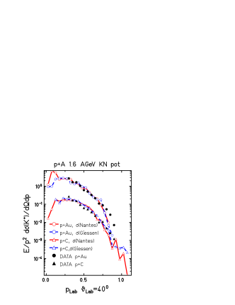
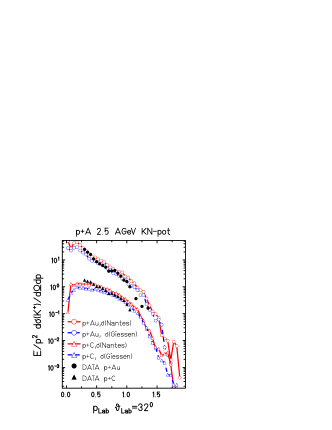
Figure 36: Influence of the different cross section parametrizations to p+C and p+Au KaoS data at 1.6 and 2.5 GeV

Let us revisit the comparison of the p+A spectra. From fig. 36 we find a small influence of the cross sections to the spectra when regarding low energies as we can also see for forward angles on the left hand side of fig. 37. For this reaction the dominance of $NN$ channel yield on the other hand a influence of the $NN\to N\Lambda K$ channel on the spectra. If we replace our parametrization (Sibirtsev, sibirtsev ) by that of Tsushima tsu (green dash-dotted line with diamonds), we find a visible lowering of the spectrum, which now is in better agreement to the data. However we should keep in mind that for other energies the Tsushima cross section also shows deviation from the data (see right hand side of fig. 12). The parametrization of David david (black dotted line with triangles) overshoots the spectra obtained with the Sibirtsev cross sections while the refitted parametrization of David (cyan line with triangles) shows again a spectrum comparable to that obtained with the Sibirtsev cross section.

However the effect is increasing with energy (see right hand side of fig. 36 and right hand side of fig. 37). At these higher energies the effect of the optical potential is decreasing. Therefore there might be a chance to see the potential at low energies. However we have to remember the influence of the Fermi momentum. A significant reduction of the Fermi momentum enhances the contribution of the $N\Delta$ channel and thus the influence of its cross section uncertainties.

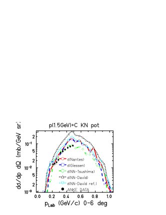
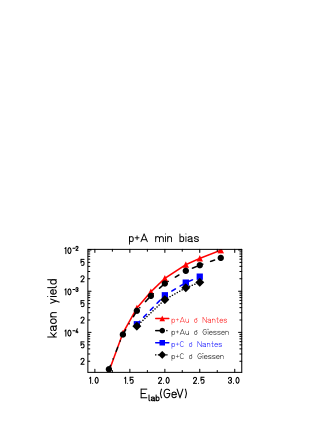
Figure 37: Influence of the different cross section parametrizations to p+C ANKE data at 1.5 GeV (left) and excitation function of the kaon yield (right)

However we have to keep in mind that the rescattering influences the spectra, especially at forward angles.

V.6 Influence of the cross section uncertainties on A+A results

As we have already seen in fig. 35 there is a strong influence of the uncertainties of the cross section in A+A collisions. This influence is most prominent where the contribution of the $N\Delta$ channel is largest.

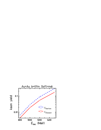
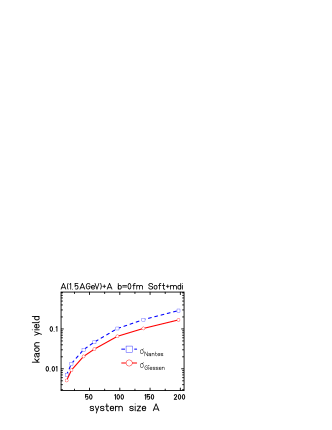
Figure 38: Excitation function (left) and system size dependence (right) of the kaon yield with and without KN-potential.

Fig. 38 shows the excitation function of Au+Au (left hand side) and the system size dependence at 1.5 AGeV (right hand side) for both cross section parametrizations. We see that all the time the calculations using the Giessen cross sections (full lines) yield less kaon than the calculations with the Nantes cross sections. The difference is smaller for smaller systems which corresponds to a smaller contribution of the $N\Delta$ channel. However the difference is also smaller at lower energies although here the contribution of the $N\Delta$ channel is higher. This effect is caused by the parametrizations themselves which show a larger discrepancy for high $\sqrt{s}$. This high values of $\sqrt{s}$ are only available at high incident energies.

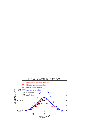
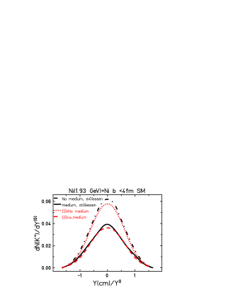
Figure 39: Comparison of FOPI data to different microscopic calculations and the contribution of the different cross section parametrizations.

Fig. 39 shows on the left hand side a comparison sqm2001 of experimental data of the FOPI rit and KaoS collaboration menzel with calculations from Giessen (RBUU) cassing and Nantes (IQMD) which puzzled the kaon community for a while. While our calculations (blue lines) can reproduce the data by assuming a kaon optical potential (full blue line), the Giessen results (red lines) could only explain the data when calculating without an optical potential (red dotted line). The right hand side of fig. 39 reveals the effect of the $N\Delta$ cross section to this puzzle. When using the same cross section parametrization as the Giessen group, our IQMD calculations (black curves) reproduce nearly the Giessen curves (red curves) as well with as without optical potential.

This example illustrates that the uncertainty on the cross section of inaccessible channels still is an important constraint on the understanding of the experimental results on kaon production. It should be repeated that the Giessen group has changed its cross section parametrizations in the mean time and now also reproduces the Ni data with an optical potential.

V.7 Influence of delta lifetime and nucleon-nucleon cross sections on the kaon production in A+A collisions

Let us finally investigate the influence of the delta lifetime on the kaon yield in A+A collisions. Here the delta channel is much more important as we have already seen in the discussion of the uncertainties of the $N\Delta$ production cross section.

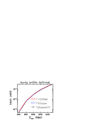
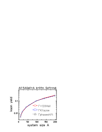
Figure 40: Excitation function (left) and system size dependence (right) of the kaon yield with different delta lifetimes.

Fig. 40 shows the excitation function (left) and system size dependence (right) of the kaon yield with different delta lifetimes: a fixed lifetime of 120 MeV (red full line), the Kitazoe parametrization (blue dashed line) and the phase-shift parametrization (black dotted line). All parametrizations yield quite the same yields, the fixed width having slightly higher values. This corresponds to the effect that Kitazoe and phase-shift parametrization do not very much differ for high mass deltas, while the fixed value allows a longer lifetime of the high mass delta before it decays. High mass delta have a better chance for having sufficient energy for producing a kaon.

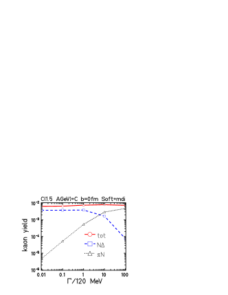
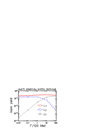
Figure 41: Dependence of the kaon yield on the delta lifetime for C+C (left) and Au+Au (right)

A reason of the quite similar yields is the counterbalance of delta involved and pion involved channels. Fig. 41 shows the dependence of the kaon yield (red full line) on the (fixed) value of $\Gamma$ for C+C (left) and Au+Au (right). Changing $\Gamma$ to smaller values means enhancing the delta lifetime and thus allowing the delta for a longer time to test collisions with nucleons. Enhancing $\Gamma$ reduces the disponibility of the delta in the reaction zone and thus reduces the kaon production via the $N\Delta$ channel (blue dashed line). On the other hand, the pions are emitted earlier and thus can better produce kaons via $\pi N$ collisions when the system is still dense. Both effects compensate over a large scale in the delta lifetime.

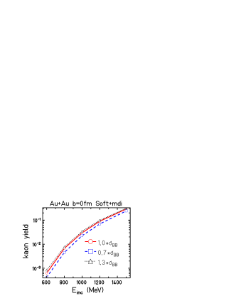
Figure 42: Excitation function (left) and system size dependence (right) of the kaon yield with different factors to the nucleon-nucleon cross section.

Let us finally study the influence of scaling the total nucleon-nucleon cross section but leaving the kaon production cross section unchanged. Fig. 42 shows the corresponding excitation function (left) and system size dependence (right) for calculations with an unscaled cross section (red full line), a cross section reduced by a factor of 0.7 (blue dashed line) and a cross section enhanced by a factor of 1.3 (black dotted line). A reduced cross section (blue dashed line) yields less stopping and reduces the number of particles equilibrated in the high density region. These particles are the major producers of kaons. Therefore a reduction of the kaon number is found. The opposite effect is seen for the enhancement of the nucleon-nucleon cross section (black dotted line) which enhances the kaon number. However, the effects are still moderate since the nucleons have still a possibility to undergo a high number of collisions. Finally it should be reminded that also the properties of the nucleus like a change in the Fermi momentum has a visible effect on the kaon yield as it has already been shown in fig. 26.

VI Kaons and the nuclear eos

As we have seen, there are two major problems on fixing the equation of state by looking on the kaon multiplicities which are the influence of the optical potential and the uncertainties of the cross sections. We will soon discuss a method for resolving this problem but first do some considerations on $K/A$ scaling.

VI.1 K/A scaling

As we have already seen, the number of kaons is depending on the size of the participating system. In central collisions all particles of both nuclei are participating, in peripheral collision one has to describe the number of participants by e.g. a geometrical model. Our calculations here are performed with b=0, thus the number of nucleons $A$ in one nucleus is equal to the number of participating nucleons and half the total participant number.

If we scale the number of kaons by the system size $A$ and plot its dependence on A in a double-logarithmic representation, a linear graph of a slope $m$ would correspond to a scaling law of the type

$$N(K)\propto A^{1+m}$$ (24)

For a flat curve $m=0$ the number of kaons is directly proportional to the total number of nucleons. We may assume that the kaons are produced in the whole volume of the reactions. For negative $m=-1/3$ we may assume that the kaons are only produced at the surface and scale with the number of nucleons at the surface. For a positive number $m>0$ we may assume a collective production of the kaons, requiring a high density. This would be of interest when searching for an effect of the nuclear equation of state, i.e. an observable focusing on high densities.

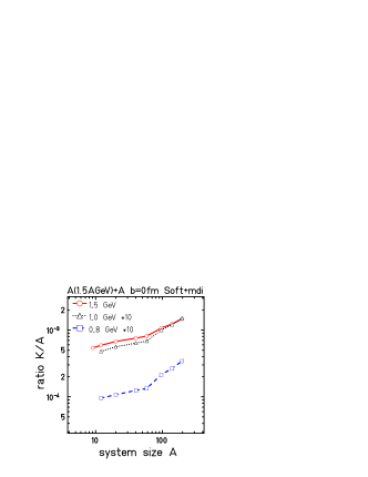
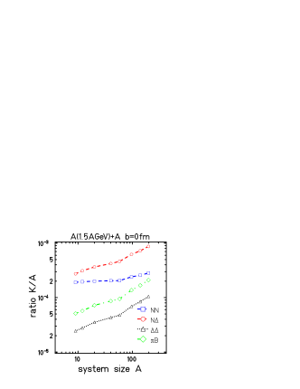
Figure 43: System size dependence of the $K/A$ ratio in b=0 collisions at different energies (left) and contributions of the different channels (right) in double-logarithmic representation.

Fig. 43 shows the system size dependence of $K/A$ in a double logarithmic representation. We see that the curves are not linear. Thus, a direct $A^{1+m}$ scaling is not possible. Nevertheless, the curves are continuously rising, giving significance for collective production. The curve for 0.8 GeV at the left hand side  (blue dashed line) increases stronger than the curve for 1.5 GeV (red full line), showing that the collectivity is more important at low energies than at high energies. The right hand side shows the scaling for different channels at an energy of 1.5 AGeV. The $NN$-channel (blue dashed line) is nearly flat. Here we are nearby the threshold so that we could nearly produce a kaon in each collision of a projectile and a target nucleon. The $N\Delta$ channel (red full line) and $\Delta\Delta$ channel (black dotted line) show a stronger increase. This is in agreement with the previous findings that these channels require many previous collisions and take place at high densities.

Let us now look on the centrality dependence of kaon production in collisions at 1.5 AGeV. This analysis differs to the previous analysis performed at $b=0$fm where one could imagine that all nucleons were actively participating in the collision. In less central collision we have to differentiate between participating nucleons and spectators. This distinction is not unique and depends on the criteria one may use to define a participant. Here we will use the geometrical model which relates the impact parameter directly to a number of participants. The relation is shown on the left hand side of fig. 44.

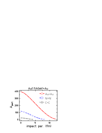
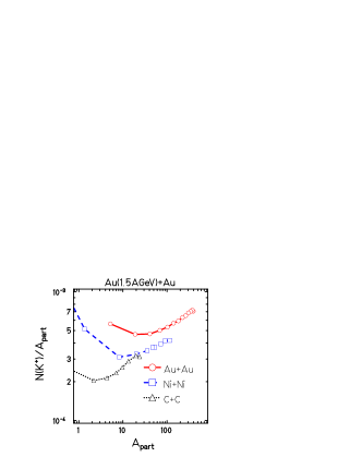
Figure 44: Participant number as function of the impact parameter (left) and kaon number per participant as function of the participant number (right) for Au+Au, Ni+Ni and C+C

The right hand side of fig. 44 shows the dependence of the ratio $N(K^{+})/A_{part}$ as a function of $A_{part}$ for the systems Au+Au (red full line), Ni+Ni (blue dashed line) and C+C (black dotted line) in double logarithmic representation. We see that all curves show a positive slope for central collisions but a negative one for very peripheral collisions. This effect might be due to surface effects and problems in defining participants at very central collisions. We will therefore skip the peripheral collisions in the following.

We also find that the slopes of C+C could be continued to Au+Au. However, the curves of Ni+Ni ly a little bit below which corresponds to the edge structure seen on the left hand side of fig. 43 where this system already showed some different behavior. We therefore plot the values of different systems into one graph a try to fit it with one global slope. In order to avoid problems with peripheral collisions we require events with a participant number that is at least a quarter of the maximum participant number $A_{part}>0.25A_{part}^{max}=0.5A$.

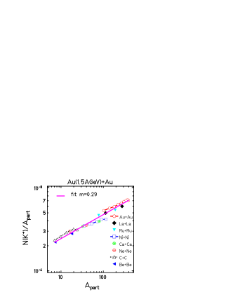
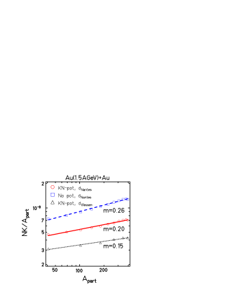
Figure 45: Participant number dependence of the kaon yield for non-peripheral collisions of different systems (left) and influence of potential and production cross section (right)

Fig. 45 shows on the left hand side  that all the kaon numbers of different events could be roughly fitted by one function with $N(K^{+})\propto A^{1.29}$. This clearly signifies the existence of collective effects for the kaon production.

This slope may depend on different ingredients as we can conclude from the right hand side of fig. 45 where we plot the centrality dependence in Au+Au for calculations with different options for the KN optical potential and the production cross section. If we use the Nantes cross section parametrization and switch off the potential (blue dashed line) we enhance the slope parameter $m$ from 0.20 (with potential, red full line) to 0.26. This corresponds to the effect that the optical potential penalizes especially at high densities, which are most important for kaon production. When changing the cross section parametrization to the Giessen type (black dotted line) we reduce $m$ to 0.15. Here we reduce the contribution of the $N\Delta$ channel which has a stronger slope than the $NN$ channel as we have seen on the right hand side of fig. 43.

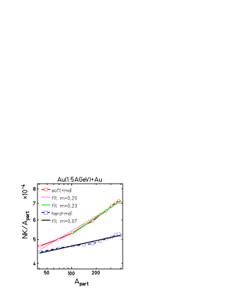
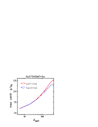
Figure 46: Participant number dependence of the kaon yield (left) and of the maximum central density (right) for a hard and a soft equation of state

Finally the equation of state has also a strong effect on the slope parameter $m$ as we can see in fig. 46 where we compare calculations with a hard (blue dashed line) and a soft (red full line) equation of state. The hard equation of state has a small value of $m=0.07$ while the soft equation of state has a higher value $m=0.20$ which still increase to $m=0.23$ when we apply the condition $A_{part}>0.25A_{part}^{max}=0.5A$. At small participant numbers the yields of hard and soft equation of state become similar. For peripheral collisions both equations of state yield about the same maximum densities while for central collisions the difference of the maximum density increases which causes a stronger rise of the kaon number.

Therefore, an analysis of the kaon data toward the dependence of the nuclear equation of state seems to be interesting.

VI.2 The effect of the nuclear equation of state on the kaon yields

Let us now look at the effect of the nuclear equation of state, when the optical potential is included. We already saw that this optical potential penalizes the kaon production especially at high densities and thus counterbalances (at least in part) the effect of the higher density reached in a soft equation of state.

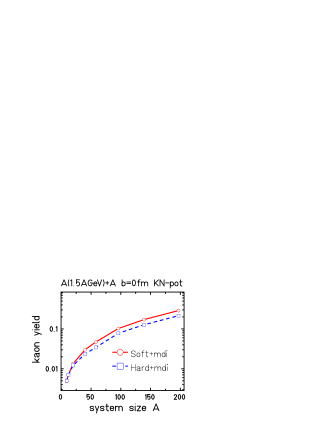
Figure 47: Excitation function and system size dependence of the kaon production with KN potential for a hard and a soft potential.

Fig. 47 compares the effect of the nuclear equation of state and the kaon yield. We see a slight enhancement of the kaon number when a soft equation of state is used (red full line). This enhancement can be found at all energies analyzed here but should vanish at energies far above the threshold. The effect of the equation of state is strongest for big systems and vanishes at small systems like C+C.

In order to explain this effect we analyze the influence of the compressibility at lower incident energies where these effects have been found to be especially sensitive.

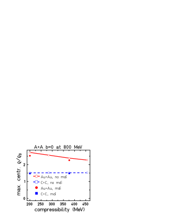
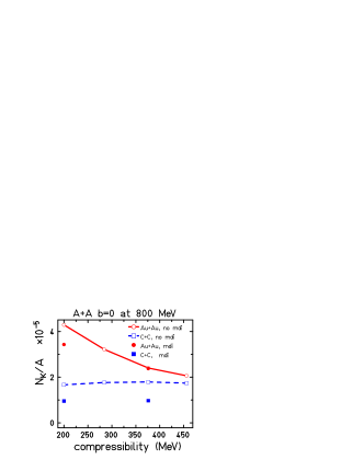
Figure 48: The maximum central density (left) and the kaon yield normalized by the system size $N_{K}/A$ (right) as a function of the compressibility for Au+Au and C+C reaction at 800 MeV incident energy

The left hand side of fig. 48 shows the maximum density reached in a central reaction in calculations of Au+Au (red full line) and C+C (blue dashed line) collisions at 800 MeV incident energy. A smaller value of the compressibility corresponds to a softer equation of state. For the heavy gold system we see a visible decrease of the density with increasing compressibility while for the light carbon system there is no effect. Furthermore the absolute values of the maximum compression are much smaller than the corresponding values of the gold system. The carbon system is too small for allowing enough compression to built up a high density region. Furthermore we see that the calculation without momentum dependent interactions (open symbols with curves) yield higher compression than the calculations including momentum dependence (full symbols). Momentum dependent interactions yield additional repulsive forces which add to the repulsion caused by the compressed matter.

The right hand side of fig. 48 shows that the kaon yield (normalized by the system size) $N_{K}/A$ shows a similar behavior. For the heavy system the kaon yield drops with increasing compressibility (and decreasing maximum density) while for the light system the yield stays constant. The effects is weaker than shown in fig. 20 since the kaon potential which is applied for the calculations in fig. 48 penalizes the production at higher densities and thus reduces the effect. Nevertheless a net effect is remaining. It should also be stated that the application of momentum dependent forces (mdi, full symbols) reduces the kaon yield additionally. This is due to the additional repulsion caused by the momentum dependent potentials. The effect is weaker for the carbon system where less compression is obtained.

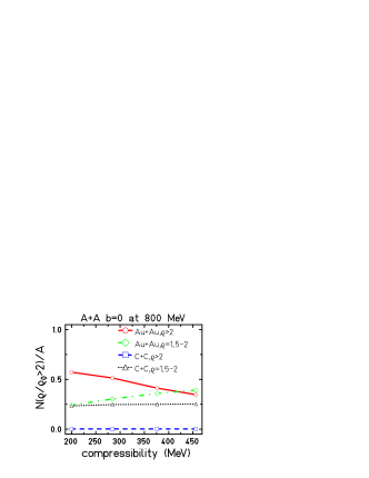
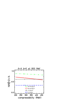
Figure 49: The fraction of particles having reached a certain maximum density (left) and having reached a minimum number of collisions (right) as a function of the compressibility for Au+Au and C+C.

In order to understand the effect of the compressibility let us look to the fraction of particles which have touched maximum density of more than twice times normal nuclear matter density. From the left hand side of fig. 49 we conclude that in heavy systems more particles enter a high density $\varrho/\varrho_{0}>2$ when using a low compressibility (red full line) while for a high compressibility more particles stay at intermediate densities ($\varrho/\varrho_{0}=1.5-2$, green dash-dotted line). For a light system there is no effect. In a high density region there is more chance for having a collision. This is especially important for deltas which have to find a collision partner before they decay. In the average they only have 2-3 fm/c of time for having a $N\Delta$ collision, which as we have seen is the major channel at lower incident energies.

Starting from the left hand side of fig. 49 it is not surprising to see on the right hand side of fig. 49 that the contribution of particles having more than 4 (red full line for the Au case and black dotted line for the C case) or at least 3 collisions (green dash-dotted line for Au and black dotted line for C) is decreasing with increasing compressibility for the Au case and staying constant for the C case. As we have already seen, kaons are predominantly produced at high densities by parents having undergone a large number of collisions. Therefore it is quite reasonable to see a strong dependence of the kaon yield on the reached density.

The different effect of the compressibility to large and small systems suggests to fix uncertainties of the production cross section on C+C where the equation of state do not show an influence. Afterward one could use the results of Au+Au for looking at the equation of state. A similar ansatz would be to look directly at the ratios of kaon numbers in Au+Au and C+C.

VI.3 Ratios of Au/C

The KaoS collaboration has proposed to analyze the ratio of the kaon numbers in Au+Au and C+C sturm ; Sturm in order to search for the nuclear equation of state. The basic idea is that all uncertainties on the optical potential and the cross sections should drop out that way. Furthermore experimental problems of detector efficiencies, acceptance cuts, total normalization etc. could be minimized when measuring both systems with the same experimental setup.

Fig. 50 shows this ratio as a function of energy for a hard and a soft equation of state.

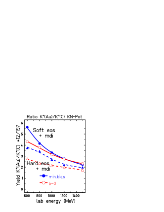
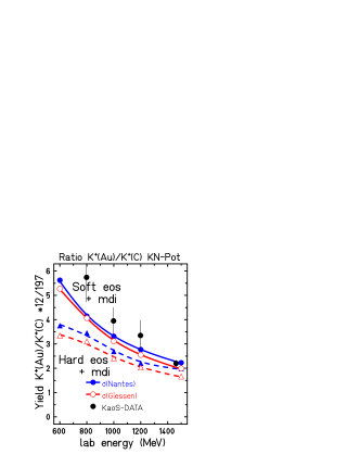
Figure 50: Kaon ratios Au/C for minimum bias and b=0 events (left) and comparison to data using different cross section parametrizations

A soft eos yielding higher kaon numbers shows higher values than a hard eos. The values become larger for lower energies. The difference between hard and soft eos also become more significant for lower incident energies. This confirms the tendency which was already seen in fig. 21 where for a calculation without potential the sensitivity to the eos was higher at 0.8 GeV than at 1.5 GeV.

Since an experiment may not measure $b=0$fm we compare on the left hand side of fig. 50 calculations with $b=0$fm (red curves) which correspond to the previous analysis with calculation using the whole impact parameter range (min. bias, blue curves). We see that both calculations show the same tendencies.

The right hand side of fig. 50 compares the minimum bias calculations with experimental data (bullets) taken by the KaoS collaboration sturm ; Sturm . The data are supporting the soft eos. In order to study possible incertitudes of the results to the cross sections, we show two calculation sets, one using our standard parametrization (Nantes, blue curves) and one using the parametrizations of the Giessen group (Giessen, red curves).

The uncertainties of the cross sections cancel in the ratio and the curves of both parametrizations are quite similar. It should be noted that similar results have also been obtained by independent groups fuchs .

Next we want to study whether the optical potential could effect this ratio.

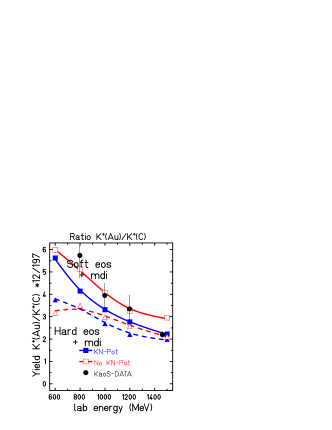
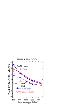
Figure 51: Kaon ratios Au/C calculated with and without KN potential compared to data (left) and influence of different delta lifetimes (right)

The left hand side of fig. 51 compares calculations with (blue curves) and without (red curves) optical potential with the KaoS data. Again the general difference between hard and soft eos remains the same. The calculations with soft eos without potential fit even better to the data.

In general this ratio seems to be quite robust. On the right hand side of fig. 51 we changed some parametrization of the delta decay changing the lifetime of the delta without changing the ratio dramatically.

Even changes in the nucleon-nucleon cross sections as shown on the left hand side of fig. 52 do not harm this ratio. When we reduce the nucleon-nucleon cross section from normal values (blue curves) to 70 % of this value (red curves) we may change the nucleon rapidity distributions, transverse flow and pion numbers significantly hart but not the Au/C kaon ratio.

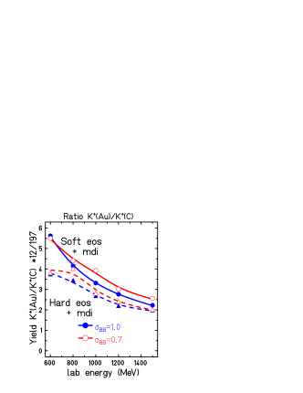
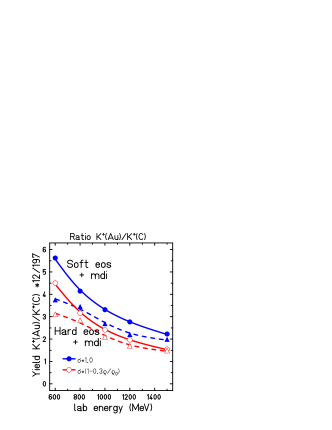
Figure 52: Kaon ratios Au/C for different cross section parametrizations for BB collisions

The only way to really harm this robust ratio is the use of density dependent nucleon-nucleon cross sections (red curves) as shown on the right hand side of fig. 52. However, these changes would yield drastic effects on all other observables. Thus, we can state that the ratio of the kaon yields in Au/C is a very robust observable supporting the soft equation of state.

VII Dynamical observables and thermal properties

After the discussion of the kaon yields we now want to describe observables of the kaon dynamics and study the influence of the optical potential and the rescattering. We shall keep in mind that for the given distributions the optical potential influences the absolute yield of the kaons and thus the absolute normalization. If we state that the optical potential influences an observable more or less significantly, the absolute yield will all the time remain a difference.

VII.1 Radial expansion

As we have seen in fig. 19 the radial density profile of the kaon production is peaked in the centre at $R=0$. The radial density of the kaons keeps this maximum during the whole reaction as it can be seen on the left hand side of fig. 53 where we show snapshots of the radial density of the kaons taken at the times $t=4$ fm/c (blue dashed line), $t=8$ fm/c (red full line), $t=12$ fm/c (black dotted line), $t=16$ fm/c (green dash-dotted line) and $t=20$ fm/c (blue dotted line).

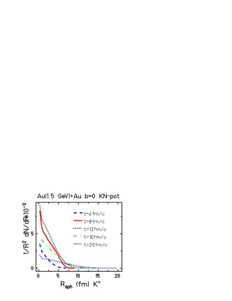
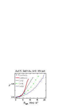
Figure 53: Time evolution of the radial density and the radial velocity profile of $K^{+}$ in Au(1.5AGeV)+Au collisions at b=0fm.

The right hand side of fig. 53 shows the corresponding radial velocity components $v_{r}=\vec{v}\cdot\vec{r}/r$ as a function of the radial distance $R$. We see that the profiles are not linear, therefore a radial expansion concept might have difficulties. Furthermore we see that the maxima of the velocities increase with time. This may be due to an acceleration of the kaons caused by the repulsive optical potential.

VII.2 Kaon spectra

Let us now look at the kaon spectra. We present them in Lorentz invariant form

$$\mbox{xaxis}=E(cm)\qquad\mbox{yaxis}=\frac{E}{p^{2}}\frac{dN}{dp\quad d\Omega}$$ (25)

In this representation a thermal Boltzmann gas with the distribution

$$dN\propto e^{\frac{-E(cm)}{k_{B}T}}\,dLips\qquad dLips=\frac{d^{3}p}{E}=\frac{p^{2}\,dp\,d\Omega}{E}$$ (26)

(where $dLips$ stands for a Lorentz invariant phase space element) has a linear shape when presenting the y-axis in logarithmic scale and the slope parameter corresponds to the inverse temperature.

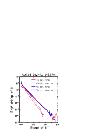
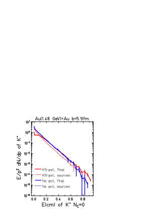
Figure 54: Comparison of initial and final spectra with and without potential.

Fig. 54 shows the temperature of semi-central collisions in a Au(1.48AGeV)+Au collision for calculations with (red curves) and without (blue curves) potential. The solid lines show the spectra taken with the final momenta of the kaons (after propagation and rescattering in the medium) whereas the dotted lines show the momenta the kaon had directly after their production (source spectra or initial spectra). For both calculations (with and without potentials) the initial spectra show similar slope at higher energies and converge at very low energies. The final spectra show higher temperatures than the initial spectra. Calculations with and without potential show different values at low energies and same values at high energies. The difference of the initial spectra at high energies corresponds to the shift of the threshold due to the potential penalty. At the final state the repulsive potential pays back this energy when the kaon enters the free mass. The regain of the energy loss in threshold can be nicely demonstrated on the right hand side of fig. 54 where initial and final spectra are shown for those particles that did not collide. For the calculations without potential initial and final spectra are the same. For the calculation with an optical potential the difference between initial and final spectra is only due to the repulsive optical potential. We see that the potential shifts the spectra back to the values of the calculation without potential. Only close to the threshold there is a lack remaining. This lack is caused by those reactions which would have been above the threshold if the potential was not there but which were forbidden by the threshold shift.

As we can see from the difference of the initial and final spectra in calculation without the optical potential of the kaons, the rescattering of the kaons plays an important role for understanding the final energy distribution.

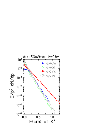
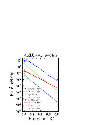
Figure 55: Comparison of the contribution from kaons that collided frequently and those who did not collide

Therefore we study in fig. 55 those kaons which did not collide (triangles) and those which did collide frequently (circles) in separate analysis. We see on the left hand side of fig. 55 that the initial spectra of the kaons without collisions (green dash-dotted line with open triangles) and of the multicolliders (black dotted line with open circles) show similar slopes. The multicolliders dominate in the absolute yield. Thus, we can conclude that this selection to the collision numbers has no bias. The final spectra are completely different. The right hand side of fig. 55 shows the same spectra multiplied with additional factors in order to disentangle the graphs. Each spectrum has been fitted by a Boltzmann ansatz as seen in eq. 26. We see that the sources show a temperature of about 84 MeV. The potential shifts the uncollided particles to a temperature of about 97 MeV. The multicolliders who underwent more than two collisions (additional to the potential repulsion) show final temperatures of about 130 MeV. Therefore, we can conclude that the collisions are giving stronger effects than the potentials.

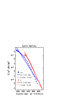
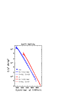
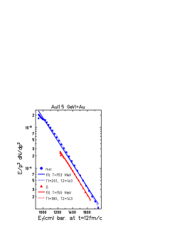
Figure 56: Time evolution of the nucleon and delta spectra

A tentative explanation of this effect is shown in fig. 56. We present the nucleon (blue curves) and delta (red curves) transverse spectra taken at the time steps $t=4$ fm/c (left), $t=8$ fm/c (middle) and $t=12$ fm/c (right). The longitudinal spectra might still be dominated by the projectile-target kinematics in this early stage of the reaction. The chosen time steps correspond to the time window of kaon production. We see that at early times the nucleons and deltas do not show a thermal spectrum that could be described with one temperature only. They will reach this equilibrated spectrum at about 16-20 fm/c. The high energy components simulate lower temperatures than the low energy components. The delta temperatures are lower than the nucleon temperatures. The production of a kaon takes place early and requires high energetic nucleons and (preferentially) deltas. Their temperatures are quite low at these early times. Therefore, the source temperature is quite low. Later on the kaons may collide with all nucleons (where there are more nucleons with low energies) and thus see the high temperature component in the collisions.

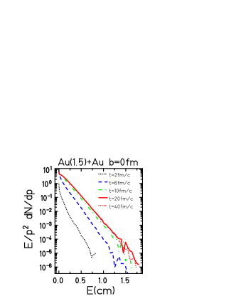
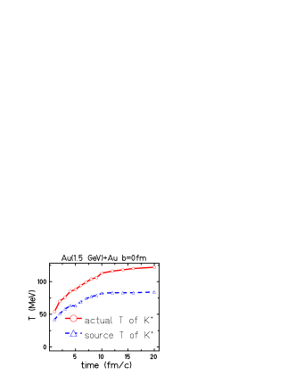
Figure 57: Time evolution of kaon spectra and temperatures

This assumption is supported by the analysis of the time evolution of the spectra. The left hand side of fig. 57 shows actual spectra at different time steps. We see a rise of the temperature in time. The right hand side of fig. 57 shows the time evolution of the source and actual temperatures. We see that both temperatures are rising in time. The source temperatures rise since up to about 12 fm/c the high energy components show rising temperatures. The rise of the actual temperatures is due to the collision in a system of nucleons which is still heating up.

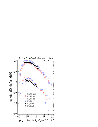
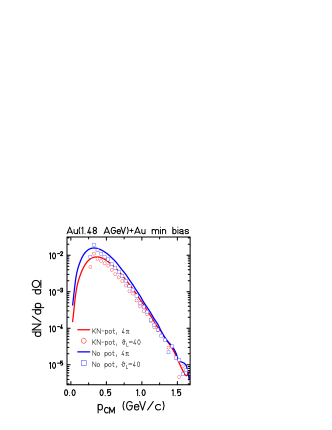
Figure 58: Comparison of lab momentum spectra and the effect of the potential on the spectra in the cm frame

Let us now compare the spectra to experimental data. The left hand side of fig. 58 compares the laboratory momenta of kaons taken at $40^{0}$ degrees with experimental data of the KaoS-collaboration foerster . Blue symbols denote calculations without potential, red symbols calculations with an optical kaon potential and the black filled symbols the KaoS data. We see a preference for the calculation with an optical potential but the differences are not very significant. This is due to the effect that unfortunately the experiment cannot measure the kaons up to lowest centre-of-mass momenta. The right hand side of fig. 58 shows the corresponding centre-of-mass spectra calculated with (red line and symbols) and without KN potential (blue line and symbols). The lines correspond to spectra obtained from full $4\pi$ analysis while the symbols correspond to spectra only in the $\vartheta_{lab}=40^{0}\pm 4^{0}$ angle. We see that the latter spectra just end at the point when the significance of the calculations becomes most prominent.

VII.3 Kaon temperatures

Let us now compare the temperatures determined by experiment with calculations of the IQMD model. The experiment divided their events in five centrality bins selected by the participant number. IQMD divides its events into the same centrality bins by direct selection of the impact parameter. A further difference is that the experiment can only use an angular segment determined by the detector position while IQMD can access the full $4\pi$ event. Furthermore the experiment can only cover a range of detectable energies. Very high and very low momenta are cut off.

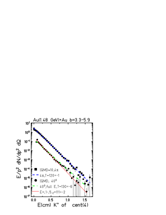
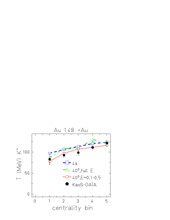
Figure 59: Determination of temperatures

Fig. 59 shows the effect of these constraints to the determination of the temperatures. Using full $4\pi$ information (blue dashed line) yields higher temperatures than observed experimentally. Reducing the event to a $\vartheta=40^{0}\pm 4^{0}$ region (green dash-dotted line) and applying additional cuts to the energy coverage (red dotted lines) yields low temperatures which are now compatible to those measured by experiment.

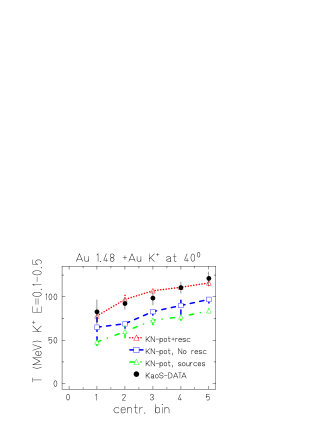
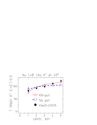
Figure 60: Comparison of temperatures to KaoS data

Finally, fig. 60 shows a comparison of $K^{+}$ temperatures (using optical potential but switching the rescattering on and off, left hand side) and in a calculation with (red dotted lines with triangles) and without (blue dashed line with squares) optical potential to the KaoS data foerster . The left hand side shows that the temperature of the initially produced kaons is much too low to explain the data and that the potentials shift up the temperatures but not sufficiently. On the other hand if we calculate with full rescattering (right hand side) but play on the potentials we end up with similar temperatures but a slightly different centrality dependence. We see that the calculations with potential show a nice agreement to the data. However, the calculations without potential are not contrary to the data.

VII.4 Energy and system size dependence

Let us shortly discuss the dependence of the inclusive spectra (i.e. taking all impact parameters) on the incident energy and on the system size

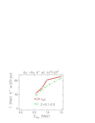
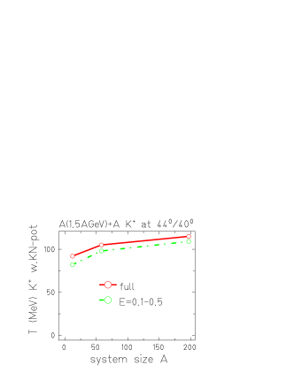
Figure 61: Excitation function and system size dependence of the temperatures at laboratory angles of $40^{0}$ or $44^{0}$.

The left hand side of fig. 61 shows the temperatures taken at laboratory angles of $44^{0}$ (0.56, 0.78 and 0.96 GeV) or $40^{0}$ (1.48 GeV). The choice of the lab angles is guided by the angles taken by the experiment. All choices correspond to kaons at mid-rapidity when going to higher laboratory momenta. We see an increase of the temperatures with the incident energy. However, there is a slight difference between the temperatures fitted to the spectra at the full energy scale and the spectra taken using an energy cut. The system size dependence on the right hand side of fig. 61 shows a slight increase of the temperatures when going to larger systems.

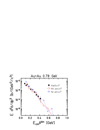
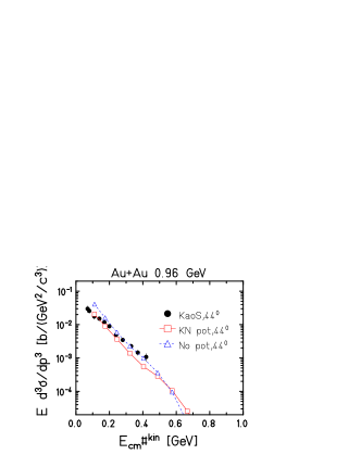
Figure 62: Comparison to KaoS data on Au+Au at lower energies

In order to estimate the fidelity of this measurement we compare the energy spectra of Au+Au collision at energies 0.78 and 0.96 AGeV. Fig. 62 shows comparison of IQMD data with KN potential (red full line) and without potential (blue dashed line) to data taken by the KaoS collaboration Laue ; Sturm We see a nice agreement to the calculations with optical potential. However the experimental temperature for the 0.96 case might be higher.

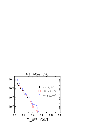
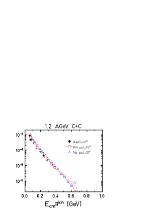
Figure 63: Comparison to KaoS data for C+C

Fig. 63 shows some comparisons for C+C at lower energies. Again the calculation with potential (red full line) seems to agree better than the calculation without potential (blue dashed line).

VII.5 Spectra at different laboratory angles

For the systems of C+C and Au at about 1.5 AGeV incident energies several laboratory angles have been measured.

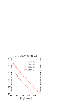
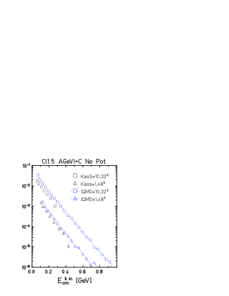
Figure 64: Invariant spectra measured at different laboratory angles for C+C at 1.5 AGeV calculated with (left) and without (right) KN potentials compared to KaoS-data

Fig. 64 compares the experimental data (black symbols Sturm ) taken for C+C at $\vartheta=32^{0}$ and $48^{0}$ to calculations of IQMD with (left hand side) and without (right hand side) KN potential. The calculation with KN potential is nearer to the data than the calculation without potential.

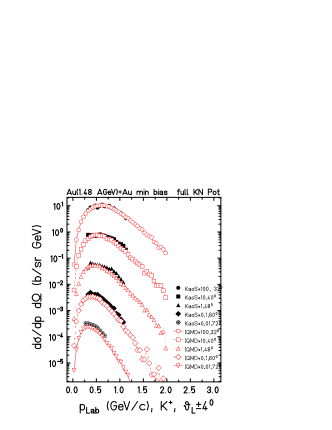
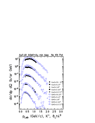
Figure 65: Momentum spectra measured at different laboratory angles for C+C at 1.5 AGeV calculated with (left) and without (right) KN potentials compared to KaoS-data

For the Au+Au data we directly compare in fig. 65 the laboratory momentum spectra taken at different angles to IQMD calculations. The data are taken by the KaoS collaboration foerster . The left hand side shows calculations with optical potential, the right hand side calculations without such a potential. We see that it is hard to decide which calculation fits better since the calculation with potential can better describe the data at smaller angles while the data at larger angles are better described by the calculation without potential. Overall IQMD has some problems in describing the full angular dependence.

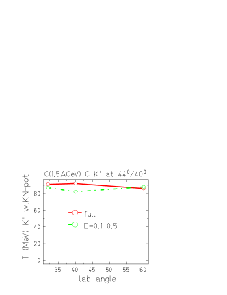
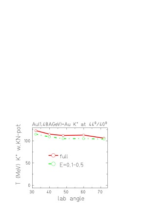
Figure 66: Temperatures of spectra measured at different laboratory angles for C+C and Au+Au at 1.5 AGeV

Fig. 66 shows the temperatures deduced from the spectra taken at different angles for C+C (left hand side) and Au+Au (right hand side). For the latter we see a slight dependence of the spectra on the lab angle. This should not be the case for an ideal isotropic thermal source. Therefore, an analysis of polar distribution would be interesting in order to see whether the source is isotropic or not.

VIII Dynamical observables and anisotropic distributions

VIII.1 Polar distributions

We now investigate the polar distributions $dN/d\cos\vartheta$, where $\vartheta=p_{Z}/p$ is the angle of the momentum vector to the beam-axis and $d\cos\vartheta=-\sin\vartheta d\vartheta$ includes the Jacobian of a polar distribution in spherical coordinates. For a better comparison of the anisotropies of the kaons in IQMD calculations to experiment foerster we divide the minimum bias (i.e. all $b$) events into two centrality bins $b<5.9$fm and $b>5.9$fm and fit the polar distributions by

$$\frac{dN}{d\cos\vartheta}=a_{0}\cdot\bigl{(}1+a_{2}\cos^{2}\vartheta\bigr{)}$$ (27)

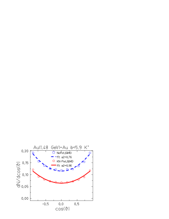
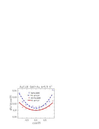
Figure 67: Polar distributions

Fig. 67 shows the corresponding distributions (symbols) and the fits (lines) for the semi-central bin ($b<5.9$fm, left hand side) and for the peripheral bin ($b>5.9$fm, right hand side). The calculations with potential are represented by red circles and their corresponding fit functions by red solid lines. The results of the fits are summarized in table 3.

centrality	$b<5.9$ fm	$b>5,9$ fm
with KN pot	0.96	1.47
without pot	0.76	2.01
KaoS data	1.1	1.9

Table 3: Comparison of the fit parameters to the angular distributions.

For semi-central collisions the calculations with the KN potential is closer to the data, while it is the opposite case for peripheral collisions. However, the IQMD-fits for peripheral collisions are dominated by the extreme bins at $\cos\vartheta\approx\pm 1$ while the other bins comply with even lower values. Thus, the polar distribution in peripheral collisions seems not be described well neither with nor without potential.

We shall therefore focus on the semi-central collisions and investigate the question, which effects are responsible for the anisotropy.

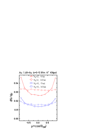
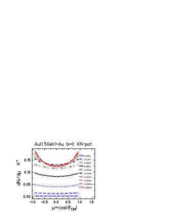
Figure 68: Time evolution of polar distributions

The left hand side of fig. 68 shows the polar distributions of kaons directly after their production (initial, dashed lines) and in the final state (final, solid lines). We selected kaons which did not collide (blue lines) and kaons which collided frequently. The initial distributions are rather flat for both types of kaons. For kaons without collisions there is a slight forward-backward enhancement due to preselection effects. Kaons have some more chance to come out in forward-backward direction without having a collision than at $\vartheta=90^{0}$. These kaons show a stronger forward-backward enhancement in the final state. This enhancement can only be true due to the optical potential since the kaons did not undergo any collision. Thus there is a visible effect of the potential to the anisotropy, which may explain the different fit parameters of the calculations with and without potential.

The multicolliding kaons (red lines) show a higher total yield and thus a higher total contribution to the kaon distribution. Furthermore they show a much stronger forward-backward peaking.We will explain this effect a few lines later.

The right hand side of fig. 68 shows snapshots of the actual polar kaon distribution at different time steps. We see that the total yield enhances to about $t=12$ fm/c without showing a very strong anisotropy. Only after the production of all kaons at times $t=12-20$ fm/c the distribution is getting its strong anisotropy. This is the time when all kaons are already produced but still collide with the nuclear matter.

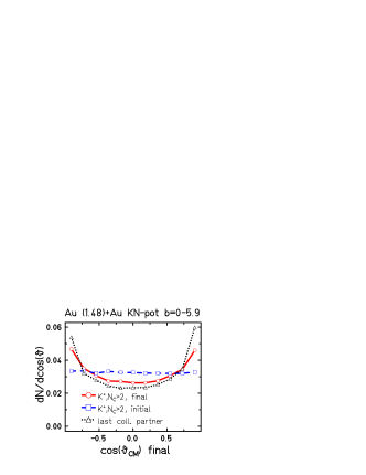
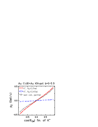
Figure 69: Contribution of the last collision partner to the the polar azimuthal anisotropy

Fig. 69 addresses the question which effect provokes the strong anisotropy for the multicollisionner particles. On the left hand side we compare the (normalized) polar distributions of the kaons directly after their production (blue dashed line), in the final state (red full line) and the distribution of the last collision partners of those particles (black dotted line). We see that the latter have a very strong forward-backward peaking, even stronger than those of the kaons in the final state. The right hand side of fig. 69 show the mean longitudinal momentum of the final kaons (red full line), the kaons directly after their production (blue dashed line) and of the last collision partners (black dotted line) as a function of the final polar angle of the kaon. The mean $p_{Z}$ of the final state (red full line) is easy to understand, since it is directly correlated to the polar angle by $\cos\vartheta=p_{Z}/p$. The mean $p_{Z}$ of the initial state after the production (blue dashed line) is zero. This means that there is no preselection from the production where the particle would go finally. Thus, particles ending in forward direction may have been produced with any longitudinal momentum initially. The mean $p_{Z}$ of the last collision partners (black dotted line) is nearly the same than the mean final $p_{Z}$. This supports the assumption that their longitudinal momentum is responsible for the final direction of the kaon. We see that the kaons have collided with a nuclear medium, which is very anisotropic in momentum space. The anisotropy is thus majorly due to the rescattering.

The influence of rescattering may also be a key for explaining the dependence of the polar distribution on the centre-of mass momentum as depicted on the left hand side of fig. 70. We know that the contribution of kaons having undergone many collisions is higher for high energy kaons than for low energy kaons. Therefore they might yield a slight enhancement of the anisotropy at high momenta.

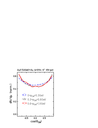
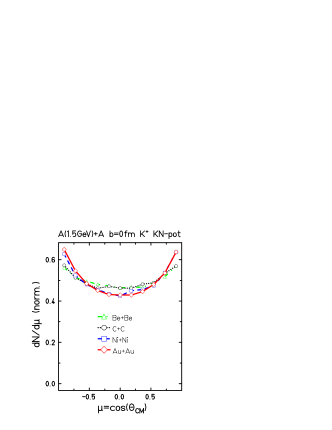
Figure 70: Polar distributions of Au+Au for different cm spectra (left) and polar distributions for different system sizes

VIII.2 Energy and system size dependence of polar distributions

Let us shortly discuss the energy and system size dependence of polar distributions. The right hand side of fig. 70 shows polar distributions of $A+A$ collisions at different system sizes. We see an enhancement of the anisotropy for heavier systems. This can again be explained by rescattering. In heavier systems there is much more rescattering of the kaons. A similar argument holds for the energy dependence of the polar distributions shown in fig. 71 for C+C (left) and Au+Au (right). At higher incident energies the nucleons show a stronger anisotropy especially for light systems. In the rescattering of the kaons they transfer some part of that anisotropy to the kaons.

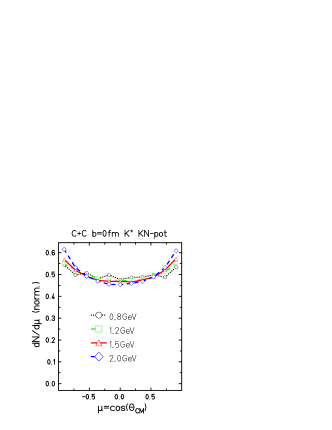
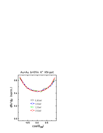
Figure 71: Polar distributions of C+C (left) and Au+Au (right) at different energies

VIII.3 Azimuthal distributions

After the investigation of the polar angle distributions let us finally study the azimuthal angular distribution at mid-rapidity. $\varphi$ is the angle between the transverse momentum $\vec{p_{T}}$ and the x-axis, where the x-axis is the direction of the impact parameter between projectile and target.

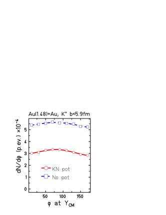
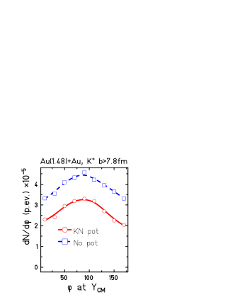
Figure 72: Azimuthal distribution for central and peripheral collisions.

Fig. 72 shows the azimuthal distribution of the kaons at mid-rapidity for a semi-peripheral centrality ($b<5.9$fm, left hand side) and for a peripheral centrality bin ($b>7.8$, right hand side). We see that calculations with an optical potential (red full line) yield less absolute yields than calculations without potential (blue dashed line) and that the distributions for semi-central events are much less pronounced than those of the peripheral events. The latter finding is also supported by experiment foerster . We will thus concentrate on the peripheral events and analyze only normalized distributions to investigate the significance of the out-of plane enhancement. The strength of the effect is in agreement with experimental data sqm2003 .

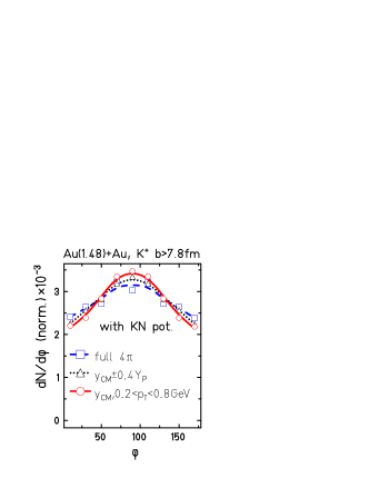
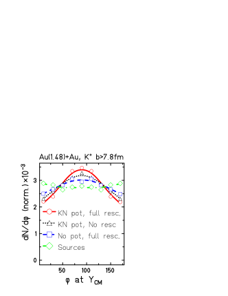
Figure 73: Contribution of cuts and of collisions

In order to understand the effect we analyze on the left hand side of fig. 73 the influence of the experimental cuts. An analysis of all kaons without any constraints on the rapidity ($4\pi$, blue dashed line) already shows an out-of-plane peak. If we now reduce the rapidity window to the same size than the experiment (black dotted line) we enhance the peak since we go more to the mid-rapidity region. If we finally apply $p_{T}$ cuts (red full line) we enhance the peak still more since we cut out rather isotope low energy kaons.

The right hand side of fig. 73 compares the distribution taking all experimental cuts but varying on the potentials and rescattering. If we forbid all potentials and rescattering (sources, green dash-dotted line) the distribution is quite flat. If we now allow rescattering but forbid the optical potential (No pot, full resc., blue dashed line) we get an enhancement out-of-plane. If on the other hand we allow the optical potential but forbid the rescattering (KN pot, No resc., black dotted line) the enhancement is stronger. But the maximum final enhancement can only be got by allowing potential and rescattering (KN pot, full resc. red full line).

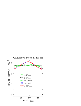
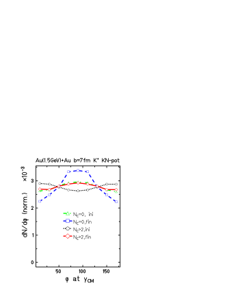
Figure 74: Time evolution of the azimuthal distribution (left) and initial and final distributions of the kaons selected according to their collision number

Let us now look on the time evolution of the kaon squeeze as it is shown on th left hand side of fig. 74. The curves are normalized, thus the effect of the increasing number of kaons is not visible. We see that the kaons are produced rather isotropically since up to about 8 fm/c there is a flat distribution which changes slightly at about 12 fm/c (when the kaon production is majorly finished) to obtain its final form at about 16 fm/c. At this time the collisions are still active. If we decompose the kaon distributions according to their number of collisions (right hand side of fig. 74) we find an effect of preselection. The initial curve of kaons that won’t collide during the reaction (green dash-dotted line) shows already a weak peaking out-of plane, while the initial curve of kaons which will collide frequently (black dotted line) has its maximum in plane. This is due to the effect that the kaons have more chance to collide when passing upward or downward into the spectator matter while the chance to escape without collisions is higher when moving out of plane. The final distributions show both an out-of-plane peak where the peak of the particles which did not collide (blue dashed line) is stronger that that of the particles which collided frequently (red full line). We see that the out-of-plane squeeze is due to rescattering and potential, where the potential seems to play the more important role.

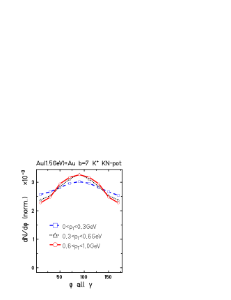
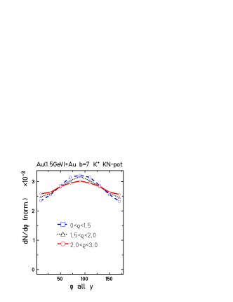
Figure 75: Azimuthal distributions averaged over all rapidities selected according to the transverse momentum (left) and the production density (right)

Let us now decompose the spectra according to the transverse momentum(left hand side of fig. 75). For a better statistics all rapidities are taken, which causes a slight reduction of the squeeze signal (see left hand side of fig. 73). We see that the squeeze is stronger for particles with high transverse momenta. This is in agreement with experimental data foerster who also noted this effect. We also decompose the squeeze according to the production density of the kaons (right hand side of fig. 75). Kaons stemming from less high densities (blue dashed line) show a stronger signal than those stemming from high densities (red full line). This is in analogy to what one finds for the nucleon squeeze hart .

VIII.4 Energy and system size dependence of the azimuthal distributions

Let us finally take a glance at the energy and system size dependence as shown in fig. 76. We see a slight increase of the squeeze effect with increasing system size and a slight decrease of the squeeze with increasing incident energy. This effect is similar but stronger for the nucleon signal which also shows an increase with system size and an decrease with incident energy for energies higher than 400 MeV. Furthermore the kaon squeeze at energies of about 1 GeV and below is dominated by the KN-potentials. Calculations including KN potentials give similar resulats with and without KN rescattering. Switching off the KN potentials reduces the kaon squeeze significantly when rescattering is allowed and yields a flat distribution without KN rescattering. This again gives some hint to the strong correlation of nucleonic matter to the dynamics of kaons.

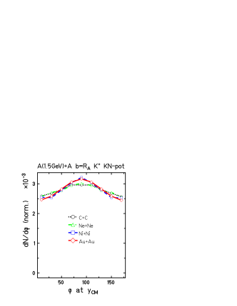
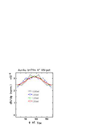
Figure 76: System size dependence (left) and dependence on the incident energy (right)

IX Conclusion

We have analyzed the production of kaons in heavy ion collisions at incident energies below the elementary threshold. We see that the production of the kaons is rather collective phenomenon requiring high densities and multi-step processes. Nevertheless the kaons do not take a unique signature of this high density zone since they rescatter afterward.

The optical potential of the kaon in the nuclear medium influences strongly the absolute number of the kaon yield and the low energy part ob the kaon spectra. There is also a strong influence on the azimuthal distributions but only a weak influence on the polar distributions.

The rescattering influences the high energy part of the spectra and the temperatures. There is a strong influence on the polar distributions but a less strong influence on the azimuthal distributions.

The comparison of absolute kaon yield between experiment and calculations is still problematic due to the uncertainties relying in the parametrization of unknown cross sections. Comparison of the spectra in p+A collisions nearby the threshold support rather the calculations with an optical potential. The use of ratios Au/C allow to cancel at least the major parts of that uncertainties and support the assumptions of a soft nuclear equation of state. This equation of state is also supported by the analysis of the dependence of the kaon yield on the participant number.

All in all we can conclude that the study of different observables on kaon production is a very helpful tool to view inside the dynamics of heavy ion collisions. IQMD is able to describe the kaon data reasonably well. In general the calculations using an optical potential and rescattering show the best agreement. This can be seen as a hint to the importance of medium effects for the kaon production close to the threshold.

References

- (1) C.B. Dover and G.E. Walker, Phys. Rep. 89, 1 (1982)
- (2) J. Aichelin and C.M. Ko Phys. Rev. Lett. 55 (1985) 2661
- (3) J. Randrup and C.M. Ko, Nucl. Phys. A 343, 519 (1980).
- (4) R. Barth et al., (KaoS Collaboration), Phys. Rev. Lett. 78 (1997) 4007.
- (5) L. Ahle et al., (E802 Collaboration), Phys. Rev. C58 (1998) 3523.
-
(6)
J. Schaffner et al, Phys. Lett. B334 (1994) 268;
J. Schaffner-Bielich et al., Nucl. Phys. A625;
(1997) 325 J. Schaffner-Bielich et al., Nucl Phys A669 (2000) 153 -
(7)
W. Cassing et al., Nucl. Phys. A614 (1997) 415;
W. Cassing and E. Bratkovskaya, Phys. Rep. 308 (1999) 65. -
(8)
C.M. Ko, Phys. Lett. B138 (1984) 361;
G. Q. Li and C. M. Ko, Nucl. Phys. A (1995) 460
G. Q. Li et al., Nucl. Phys.625 (1997) 415, - (9) C. Hartnack, L. Zhuxia, L. Neise, G. Peilert, A. Rosenhauer, H. Sorge, J. Aichelin, H. Stöcker, and W. Greiner. Nucl. Phys. A495, 303 (1989).
- (10) Ch. Hartnack. PhD thesis, GSI-Report 93-5 (1993).
- (11) S. A. Bass, C. Hartnack, H. Stöcker and W. Greiner. Phys. Rev. C 51 , 3343 (1994).
- (12) C. Hartnack et al., Eur.Phys.J. A1 (1998) 151.
- (13) H. Stöcker and W. Greiner. Phys. Reports 137, 277 (1986).
- (14) W. Cassing, V. Metag, U. Mosel and K. Niita. Phys. Reports 188, 361 (1990).
- (15) J. Aichelin. Phys. Reports 202, 233 (1991).
- (16) S. A. Bass J. Phys. G 28 (2002) 1543
- (17) L. G. Arnold et al. Phys. Rev. C25, 936 (1982).
- (18) G. Passatore. Nucl. Phys. A95, 694 (1967).
- (19) G. F. Bertsch and S. Das Gupta, Phys. Rep. 160, 189 (1988).
- (20) J. Aichelin, A. Rosenhauer, G. Peilert, H. Stöcker, W. Greiner. Phys. Rev. Lett. 58, 1926 (1987).
- (21) S. Hama et al. Phys. Rev. C41, 2737 (1990).
- (22) Ch. Hartnack and J. Aichelin Phys. Rev. C49, 2801 (1994).
- (23) M. Bleicher, UFTP Frankfurt, private communication.
- (24) C. Hartnack, J. Jaenicke, L. Sehn, H. Stöcker, J. Aichelin, Nucl. Phys. A 580, 643 (1994).
- (25) Ch. Hartnack, J. Aichelin, H. Stöcker and W. Greiner, Phys. Rev. Lett. 72, 3767 (1994).
- (26) W.J. Hogan, Phys. Rev. 166 (1968) 1472
- (27) A. Sibirtsev et al. Phys. Lett. B 359 (1995) 29
-
(28)
K. Tsushima et al., Phys. Lett. B337 (1994) 245
Phys. Rev. C 59 (1999) 369 (nucl-th/9801063) - (29) C. David et al, Nucl. Phys A 650 (1999) 358
- (30) J.T. Balewski et al. nucl-ex/9803003
- (31) B. Hong et al., Phys. Rev. C 66 (2002)034901
- (32) O.N. Hartmann, PhD thesis, TU Darmstadt 2003,
-
(33)
M. Büscher et al. Phys. Rev. C 65 (2002) 14603
M. Büscher and N. Nekipelov, proceedings of the Meson 2002, p.179. - (34) W. Scheinast, PhD thesis, University of Dresden (2004).
- (35) M. Menzel et al., (KaoS Collaboration), Phys. Lett. B 495 (2000) 26; M. Menzel, Dissertation, Universität Marburg, 2000.
- (36) J. Cleymans, H. Oeschler and K. Redlich, Phys. Lett. B485 (2000) 27.
- (37) H. Oeschler, proceedings of “Strangeness 2000”, Berkeley, USA, July 2000; J. Phys. G: Nucl. Part. Phys. 27 (2001) 1.
- (38) M.F.M. Lutz et al., nucl-th/0112053
- (39) C. Hartnack and J. Aichelin, J. Phys. G 28 (2002) 1649
- (40) C. Hartnack and J. Aichelin, J. Phys. G 30 (2004) 531
- (41) S. Pal, C.M. Ko and Z. Lin, Phys. Rev. C 64 (2001) 042201
- (42) A. Förster (KaoS Collaboration), PhD thesis, TH Darmstadt; A. Förster et al. Phys. Rev. Lett. 31 (2003) 152301; A. Förster et al. J. Phys. G. 30 (2004) 393
- (43) F. Laue et al., (KaoS Collaboration), Phys. Rev. Lett. 82 (1999) 1640.
- (44) J.L. Ritman et al.,Z. Phys. A352 (1995) 355
- (45) C. Sturm et al (KaoS Collaboration), Phys. Rev. Lett. 86 (2001) 39
-
(46)
C. Sturm, PhD thesis, TH Darmstadt
C. Sturm et al (KaoS Collaboration), J. Phys. G 28 (2002) 1895 - (47) C. Fuchs et al. Phys. Lett B 434 (1998) 245 ; C. Fuchs et al. Phys. Rev. Lett 86 (2001) 1794; C. Fuchs et al. J. Phys. G 28 (2002) 1615