Electroweak quasielastic response functions in nuclear matter

Abstract

Quasielastic electromagnetic and parity-violating electron scattering response functions of relativistic nuclear matter are reviewed. The roles played by the Hartree-Fock field and by nuclear correlations in the Random Phase Approximation (treated within the continued fraction scheme) are illustrated. The parity-violating responses of nuclei to polarized electrons are also revisited, stressing in particular the crucial role played by the pion in the nuclear dynamics. Finally, some issues surrounding scaling and sum rules are addressed.

Content

• I. Introduction

• II. Quasielastic response functions for inclusive electron scattering

  • A. Response functions

  • B. Non-relativistic vs relativistic kinematics

  • C. Free response

  • D. Hartree-Fock response

  • E. Random phase approximation response

  • F. Effective particle-hole interaction

  • G. Testing the model

• III. Parity-violating electron scattering

  • A. The asymmetry, the currents and the RFG responses

  • B. The role of the pion and other mesons

  • C. The axial response and the asymmetry

• IV. Scaling and sum rules

• V. Outlook and perspectives

I Introduction

Traditionally, studies of excitations of the nucleus via the interactions between leptons and the nucleus have been centered mostly on the longitudinal ($R_{\text{L}}$) and transverse ($R_{\text{T}}$) nuclear response functions explored in unpolarized, inelastic, inclusive $(e,e^{\prime})$ electron scattering. The present paper will also be largely restricted to the investigation of these quantities, although the set of experimentally accessible responses is much larger, including also semi-inclusive responses and responses that arise when initial or final hadronic degrees of freedom are active. In the former, particles are detected in coincidence with the scattered electron $((e,e^{\prime}p),$ $(e,e^{\prime}n),$ $(e,e^{\prime}pn),$ etc.), whereas the latter includes reactions such as ${\vec{A}}(e,e^{\prime}),$ $A(e,e^{\prime}{\vec{p}}\ ),$ etc. Of course, in all cases the incident electron may also be polarized. A concerted effort is presently being placed on experimental studies of this extended set of responses where special sensitivities to normally hidden aspects of nuclear structure are expected to exist. Such studies are very challenging and thus only relatively recently have they been made feasible by advances in accelerators, in developments of polarized electron beams and polarized nuclear targets, and in the construction of the required hadron polarimetry. Issues still surround the inclusive unpolarized responses themselves, however, and since a successful level of understanding of the underlying nuclear dynamics would be incomplete without a coherent picture of the entire set of responses, unpolarized inclusive and semi-inclusive/polarized, the former still deserve continued study and so provide the focus for the present article.

Beyond the electromagnetic (EM: parity-conserving, vector) responses $R_{\text{L}}$ and $R_{\text{T}}$ our study will also include their parity-violating analogs $R_{\text{L}}^{\text{AV}}$ and $R_{\text{T}}^{\text{AV}}$ as well as the nuclear parity-violating axial response $R_{\text{T}^{\prime}}^{\text{VA}}$. Here AV indicates that the axial leptonic and vector hadronic currents enter; VA indicates the converse. This larger set of inclusive responses may be explored via the inclusive scattering of longitudinally polarized electrons from unpolarized nuclei, since the electron helicity asymmetry is parity-violating. The three new responses all arise from interferences between the weak neutral current (WNC) and EM current. In the cases of $R_{\text{L}}^{\text{AV}}$ and $R_{\text{T}}^{\text{AV}}$ it is the vector part of the WNC that enters and this is believed to be closely related to the EM current (in the absence of strangeness content in the nucleus these two responses are tied to $R_{\text{L}}$ and $R_{\text{T}}$); in the case of $R_{\text{T}^{\prime}}^{\text{VA}}$ it is the axial part of the WNC that enters, namely an interesting new inclusive nuclear response function.

The vector responses (the four labeled either L or T) are, of course, interesting in their own right, since disentangling them through measurements of both parity-conserving and -violating inclusive electron scattering would permit the isolation of the isoscalar and isovector contributions they contain, as will be discussed in detail later. Accomplishing this separation would represent a significant step forward in our understanding of nuclear structure: indeed, for a long time researchers have sought possible ways of “measuring” how nuclear correlations work in the isoscalar and isovector channels.

A further point worth noting is that analogous responses also play a role in the scattering of hadrons from nuclei. However, in order to interpret the experimental data properly, in addition to the response functions there one also needs a reliable description of the reaction mechanism. In fact, unlike either real or virtual photons, hadrons are mostly absorbed or scattered at the surface of the nucleus. Moreover, the hadrons disrupt the nucleus to a much larger extent than do photons, and therefore the interpretation of reactions induced by photons is generally felt to be under better control than those induced by hadrons. Moderating this statement to some degree is the fact that electron scattering is still somewhat flawed by a not yet fully satisfactory understanding of dispersive effects and of the distortion of the electron waves moving in the EM potential of the nucleus. Accurate knowledge of the nuclear response functions gained with electron scattering provides a way to test the reaction mechanisms of the models employed in hadron scattering. However, the electroweak studies do not provide all of the information we seek and in this regard it is worth noting that in some cases reactions induced by hadrons give access to nuclear responses that are not easily extracted in electron scattering, the best example in this connection being offered by the long sought after spin-longitudinal isovector response.

Turning now to the problem of modeling the nuclear response functions, in the present work we confine our attention to the quasifree region, which is well suited for a microscopic treatment in terms of nucleons and mesons, specifically in terms of the standard field theoretical techniques that we employ. Although the $\Delta$ peak may also be treated in the same framework, it will not be dealt with here to curb the length of this article. Since we are concerned with kinematical regions where relativistic effects are relevant, a good starting point for the development of our approach is given by the Relativistic Fermi Gas (RFG), a covariant model in the sense that its ingredients are the fully relativistic nucleon propagators and EM/WNC vertices. Of course the RFG misses surface and finite-size effects. First of all, these are of secondary importance in obtaining a general understanding of the scattering of electrons in the quasielastic and $\Delta$ peak domains. Secondly, they can be accounted for within the semiclassical approach, which exploits the advantages offered by the translational invariance of the RFG and yet is able to incorporate some of the physics of a finite system.

As discussed in detail later, the perturbative approach we follow requires the setting up of a nuclear mean field (Hartree-Fock, HF) and the treatment of the residual interaction effects in the fully antisymmetrized Random Phase Approximation (RPA). In addition one needs as preliminary input the nucleon-nucleon force: since we would like to view the nucleus as an interacting system of baryons and mesons, a natural choice in this connection is given by a meson-exchange interaction such as the Bonn potential, which can be cast in the framework of an effective field theory. Another preliminary problem relates to the short-range nuclear correlations induced by the violent repulsion present in the nucleon-nucleon force at small distances. A technique for their treatment is indeed available, namely the summation of the Brueckner ladder diagrams; however, it is not yet possible to employ this technique covariantly especially at high density, where on the one hand ladder diagrams are increasingly important and on the other the role of relativity cannot be ignored. In lieu of this, in a few of the results discussed in the following section we shall indicate what insight can be gained by employing a parameterization of a non-relativistic $G$-matrix based on the Bonn potential.

II Quasielastic response functions for inclusive electron scattering

As mentioned in the Introduction, in past years quasielastic electron scattering from nuclei has been the subject of intense experimental [1, 2, 3] and theoretical (see, e. g., Refs. [4]–[18]) investigations. The first aim of the theoretical studies is to test the available nuclear models; once the nuclear physics issues are well understood, one might then hope to gain insight into other aspects of the problem, for instance into the form factors of the nucleon, which can be extracted from the data with an accuracy that is strictly connected to our ability to handle the nuclear physics.

In principle, the quasifree regime is thought to be the obvious place to focus on, as one hopes that there the physical quantities of interest may be computed in a reliable way, while also in this case in practice one has to cope with significant problems. Many diverse techniques have been employed in the literature. Each of them has its own relative merits and deficiencies and clearly it would be highly desirable to be able to reach some degree of convergence in their outcomes.

In the following [19], we shall be concerned with Green’s function techniques as introduced, e. g., in Ref. [20]. This method can be, and has been, applied both to finite nuclei and nuclear matter. Here, we shall focus on nuclear matter, having in mind applications to electron scattering (that is, without the complications introduced by the reaction mechanism of hadronic probes) in a range from a few hundreds to about 1 GeV/c of transferred momentum where the quasielastic peak is far from low-energy resonances and not too much affected by finite-size effects. The use of nuclear matter reduces the computational load, thus allowing a more straightforward implementation of more sophisticated theoretical schemes than would otherwise be feasible, and this makes it easier to develop and test approximation methods that might subsequently also be utilized for calculations in finite nuclei.

Let us now briefly summarize the theoretical framework that we shall discuss in detail in the following subsections.

A first issue one has to confront in setting up the formalism concerns the treatment of relativistic effects. Kinematical effects, while obviously rather important, can be included in a straightforward way. The treatment of dynamical effects is more delicate. Two main paths have been followed in the literature, either using field theoretical methods (as done, e. g., in the Walecka model and its derivations [21]) or using potential techniques (i. e., employing phenomenological potentials truncated at some order in the non-relativistic expansion). Here we shall take the second path, but to limit the amount of material to be covered, we shall discuss only non-relativistic potentials.

The extensions necessary to include higher-order relativistic terms are discussed in Ref. [14], where the nuclear response functions have been calculated using techniques similar to the ones explained below, using as an input the relativistic Bonn potential [22] expanded in powers of $P/m_{N}$ and $q/m_{N}$ up to second order — $P$ and $q$ being the average of the incoming and outgoing nucleon momenta and the exchanged momentum, respectively. As shown in [14], the effect of these dynamical relativistic corrections is significant; indeed, the validity of that expansion at high momenta and the inclusion in that framework of short-range nucleon-nucleon correlations has yet to be explored (see, however, Refs. [14, 23, 24]).

Next, one should choose the phenomenological input potential and, in connection with this choice, attempt to cope with the problem of dealing with short-range correlations. All of the formulae given in the following sections are based on a generic one-boson-exchange potential. They can thus be used both with a bare phenomenological interaction — such as one of the Bonn potential variants — or with a one-boson-exchange parameterization of the $G$-matrix generated from some potential. The use of an effective interaction derived from a $G$-matrix is a common way of including short-range correlations. However, apart from the relativistic issue, one should be aware of possible problems due to the use of a local potential to fit non-local matrix elements. At least in a few cases discussed in the literature this does not appear to be a reason for concern [25, 26]. On the other hand, possible effects arising only in the quasielastic regime remain completely unexplored. Indeed, $G$-matrices employed in quasielastic calculations are usually generated using bound-state boundary conditions, which make them real and practically energy-independent, while in general they are both complex and energy-dependent.

Once we have fixed the effective interaction, we can proceed to consider a hierarchy of approximation schemes.

The lowest-order approximation is, of course, given by the free Fermi gas. Then, one may include mean-field correlations at the HF level (or Brueckner-Hartree-Fock (BHF) if short-range correlations are accounted for). In nuclear matter a HF calculation can be done exactly without too much effort. Later we show how a quite accurate analytic approximation can be derived, and how this is needed to combine the HF and RPA schemes. The latter is the last resummation technique we shall discuss. It should be noticed that even in nuclear matter the calculation of the antisymmetrized RPA response functions is not trivial. Indeed, most calculations, labeled “RPA” in the literature, are actually performed in the so-called “ring approximation”, where only the direct contributions are kept. For this case, in nuclear matter one gets a simple algebraic equation for the response. Here, we use the continued fraction (CF) technique to provide a semi-analytical estimate of the full RPA response (see Refs. [6] and [8] for alternative methods). Calculations with this method have been performed both in finite nuclei [4, 5] and in nuclear matter [27, 28, 14, 23], always truncating the CF expansion at first order because of the difficulty of the numerical calculations involved. We have pushed the analytical calculation far enough to yield not only a fast and accurate estimate of the first-order CF contribution, but also of the second-order one. Since the rate of convergence of the CF expansion cannot be assessed on the basis of general theorems, this is the only way of getting a quantitative grip on the quality of the approximation. As mentioned before, HF (and kinematical relativistic) effects can then be incorporated in the RPA calculation, yielding as the final approximation scheme a HF-RPA (or BHF-RPA) response function.

Of course, several many-body contributions have been left out in our analysis. However the classes of many-body diagrams discussed here already allow one to capture the main features of the quasielastic response and, since semi-analytical methods have been developed for their computation, our formalism constitutes a valid starting point for the study of other many-body effects.

A Response functions

We consider an infinite system of interacting nucleons at some density fixed by the Fermi momentum $k_{F}$. For the kinetic energies of the nucleons we can choose either relativistic or non-relativistic expressions, whereas we assume that the interactions take place through a non-relativistic potential. For the latter the following expression in momentum space is assumed

$$V(\mathchoice{{\hbox{\boldmath$\displaystyle k$}}}{{\hbox{\boldmath$\textstyle k$}}}{{\hbox{\boldmath$\scriptstyle k$}}}{{\hbox{\boldmath$\scriptscriptstyle k$}}}) = V_{0}(k)+V_{\tau}(k)\mathchoice{{\hbox{\boldmath$\displaystyle\tau$}}}{{\hbox{\boldmath$\textstyle\tau$}}}{{\hbox{\boldmath$\scriptstyle\tau$}}}{{\hbox{\boldmath$\scriptscriptstyle\tau$}}}_{1}\cdot\mathchoice{{\hbox{\boldmath$\displaystyle\tau$}}}{{\hbox{\boldmath$\textstyle\tau$}}}{{\hbox{\boldmath$\scriptstyle\tau$}}}{{\hbox{\boldmath$\scriptscriptstyle\tau$}}}_{2}+V_{\sigma}(k)\mathchoice{{\hbox{\boldmath$\displaystyle\sigma$}}}{{\hbox{\boldmath$\textstyle\sigma$}}}{{\hbox{\boldmath$\scriptstyle\sigma$}}}{{\hbox{\boldmath$\scriptscriptstyle\sigma$}}}_{1}\cdot\mathchoice{{\hbox{\boldmath$\displaystyle\sigma$}}}{{\hbox{\boldmath$\textstyle\sigma$}}}{{\hbox{\boldmath$\scriptstyle\sigma$}}}{{\hbox{\boldmath$\scriptscriptstyle\sigma$}}}_{2}+V_{\sigma\tau}(k)\mathchoice{{\hbox{\boldmath$\displaystyle\sigma$}}}{{\hbox{\boldmath$\textstyle\sigma$}}}{{\hbox{\boldmath$\scriptstyle\sigma$}}}{{\hbox{\boldmath$\scriptscriptstyle\sigma$}}}_{1}\cdot\mathchoice{{\hbox{\boldmath$\displaystyle\sigma$}}}{{\hbox{\boldmath$\textstyle\sigma$}}}{{\hbox{\boldmath$\scriptstyle\sigma$}}}{{\hbox{\boldmath$\scriptscriptstyle\sigma$}}}_{2}\ \mathchoice{{\hbox{\boldmath$\displaystyle\tau$}}}{{\hbox{\boldmath$\textstyle\tau$}}}{{\hbox{\boldmath$\scriptstyle\tau$}}}{{\hbox{\boldmath$\scriptscriptstyle\tau$}}}_{1}\cdot\mathchoice{{\hbox{\boldmath$\displaystyle\tau$}}}{{\hbox{\boldmath$\textstyle\tau$}}}{{\hbox{\boldmath$\scriptstyle\tau$}}}{{\hbox{\boldmath$\scriptscriptstyle\tau$}}}_{2}$$ (2)

$$\quad+V_{t}(k)S_{12}(\hat{\mathchoice{{\hbox{\boldmath$\displaystyle k$}}}{{\hbox{\boldmath$\textstyle k$}}}{{\hbox{\boldmath$\scriptstyle k$}}}{{\hbox{\boldmath$\scriptscriptstyle k$}}}})+V_{t\tau}(k)S_{12}(\hat{\mathchoice{{\hbox{\boldmath$\displaystyle k$}}}{{\hbox{\boldmath$\textstyle k$}}}{{\hbox{\boldmath$\scriptstyle k$}}}{{\hbox{\boldmath$\scriptscriptstyle k$}}}})\mathchoice{{\hbox{\boldmath$\displaystyle\tau$}}}{{\hbox{\boldmath$\textstyle\tau$}}}{{\hbox{\boldmath$\scriptstyle\tau$}}}{{\hbox{\boldmath$\scriptscriptstyle\tau$}}}_{1}\cdot\mathchoice{{\hbox{\boldmath$\displaystyle\tau$}}}{{\hbox{\boldmath$\textstyle\tau$}}}{{\hbox{\boldmath$\scriptstyle\tau$}}}{{\hbox{\boldmath$\scriptscriptstyle\tau$}}}_{2},$$

where $S_{12}$ is the standard tensor operator and $V_{\alpha}(k)$ represents the momentum space potential in channel $\alpha$. Here $V_{\alpha}(k)$ has the general form of a static one-boson-exchange potential so that in each spin-isospin channel, namely $(0,\tau,\sigma,\sigma\tau,t,t\tau)$, it is represented as a sum of contributions from different mesons, $V_{\alpha}\equiv\sum_{i}V_{\alpha}^{(i)}$. In the central channels ($0$, $\tau$, $\sigma$, $\sigma\tau$) the contribution from any meson can be expressed as the combination of a short-range (“$\delta$”) piece and a longer range (“momentum-dependent”) piece:

$$V_{\delta}^{(i)}(k) = g_{\delta}^{(i)}\left(\frac{\Lambda_{i}^{2}-m_{i}^{2}}{\Lambda_{i}^{2}+k^{2}}\right)^{\ell}$$ (4)

$$V_{\text{MD}}^{(i)}(k) = g_{\text{MD}}^{(i)}\frac{m_{i}^{2}}{m_{i}^{2}+k^{2}}\left(\frac{\Lambda_{i}^{2}-m_{i}^{2}}{\Lambda_{i}^{2}+k^{2}}\right)^{\ell},\quad\ell=0,1,2,$$ (5)

whereas in the tensor channels ($t$, $t\tau$) one has

$$V_{\text{TN}}^{(i)}(k)=g_{\text{TN}}^{(i)}\frac{k^{2}}{m_{i}^{2}+k^{2}}\left(\frac{\Lambda_{i}^{2}-m_{i}^{2}}{\Lambda_{i}^{2}+k^{2}}\right)^{\ell},\quad\ell=0,1,2.$$ (6)

In Eqs. (* ‣ II A), $g_{\delta}^{(i)}$, $g_{\text{MD}}^{(i)}$ and $g_{\text{TN}}^{(i)}$ are the (dimensional) coupling constants of the $i$-th meson, $m_{i}$ is its mass and $\Lambda_{i}$ the cut-off; more generally, potentials without form factors or with monopole or dipole form factors are allowed.

Our starting point [29, 30, 31] is the Galitskii-Migdal integral equation for the particle-hole (ph) four-point Green’s function,

$$G^{\text{ph}}_{\alpha\beta,\gamma\delta}(K+Q,K;P+Q,P)=-G_{\alpha\gamma}(P+Q)\,G_{\delta\beta}(P)\,(2\pi)^{4}\delta(K-P)$$ (7)

$$+iG_{\alpha\lambda}(K+Q)\,G_{\lambda^{\prime}\beta}(K)\int\frac{d^{4}T}{(2\pi)^{4}}\Gamma^{13}_{\lambda\lambda^{\prime},\mu\mu^{\prime}}(K+Q,K;T+Q,T)\,G^{\text{ph}}_{\mu\mu^{\prime},\gamma\delta}(T+Q,T;P+Q,P),$$ (8)

(9)

diagrammatically illustrated in Fig. 1. In Eq. (9), $G$ represents the exact one-body Green’s function, whereas $\Gamma^{13}$ is the irreducible vertex function in the ph channel.

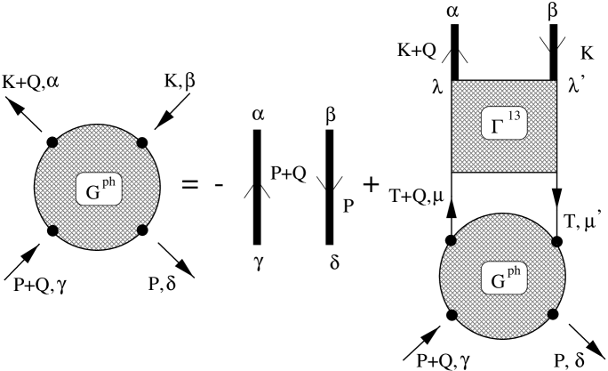
FIG. 1.: Diagrammatic representation of the Galitskii-Migdal integral equation for the ph Green’s function, $G^{\text{ph}}$; $\Gamma^{13}$ is the irreducible vertex function in the ph channel; the heavy lines represent the exact one-body Green’s functions.

Given $G^{\text{ph}}$ one can then define the polarization propagator

$$\Pi_{\alpha\beta,\gamma\delta}(Q) \equiv \Pi_{\alpha\beta,\gamma\delta}(q,\omega)$$ (10)

$$= i\int\frac{d^{4}P}{(2\pi)^{4}}\frac{d^{4}K}{(2\pi)^{4}}G^{\text{ph}}_{\alpha\beta,\gamma\delta}(K+Q,K;P+Q,P),$$ (11)

whose diagrammatic representation is displayed in Fig. 2. Note that for $\Pi(q,\omega)$ one cannot in general write down an integral (or algebraic) equation.

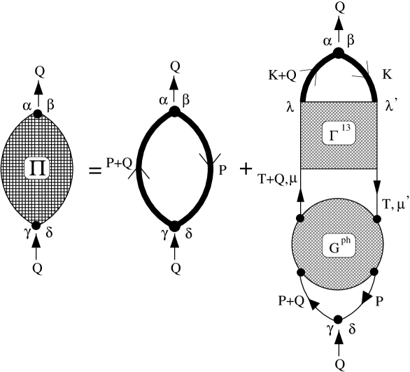
FIG. 2.: Diagrammatic representation of the polarization propagator $\Pi$ derived from the ph Green’s function $G^{\text{ph}}$.

In the case of electron scattering, one can define charge — or longitudinal — and magnetic — or transverse — polarization propagators. These, in the non-relativistic regime, read

$$\Pi^{I}_{\text{L}}(q,\omega)=\text{tr}[\hat{O}^{I}_{\text{L}}\hat{\Pi}(q,\omega)\hat{O}^{I}_{\text{L}}]$$ (13)

$$\Pi^{I}_{\text{T}}(q,\omega)=\sum_{ij}\Lambda_{ji}\Pi^{I}_{ij}(q,\omega),\qquad\Pi^{I}_{ij}(q,\omega)=\text{tr}[\hat{O}^{I}_{\text{T};i}\hat{\Pi}(q,\omega)\hat{O}^{I}_{\text{T};j}]$$ (14)

$$\phantom{\Pi^{I}_{\text{T}}(q,\omega)=\sum_{ij}\Lambda_{ji}\Pi^{I}_{ij}(q,\omega),}\qquad\,\Lambda_{ij}=(\delta_{ij}-\mathchoice{{\hbox{\boldmath$\displaystyle q$}}}{{\hbox{\boldmath$\textstyle q$}}}{{\hbox{\boldmath$\scriptstyle q$}}}{{\hbox{\boldmath$\scriptscriptstyle q$}}}_{i}\mathchoice{{\hbox{\boldmath$\displaystyle q$}}}{{\hbox{\boldmath$\textstyle q$}}}{{\hbox{\boldmath$\scriptstyle q$}}}{{\hbox{\boldmath$\scriptscriptstyle q$}}}_{j}/q^{2})/2,$$ (15)

where, for brevity, the dependence upon the spin-isospin indices has been represented in matrix form, introducing hats to indicate matrices. In Eqs. (2), $I$ labels the isospin channel and the longitudinal and transverse vertex operators are given by:

$$\left\{\begin{array}[]{l}\hat{O}^{I=0}_{\text{L}}=1/2\\ \hat{O}^{I=1}_{\text{L}}=\tau_{3}/2\end{array}\right.\qquad\qquad\left\{\begin{array}[]{l}\hat{O}^{I=0}_{\text{T};i}=\sigma_{i}/2\\ \hat{O}^{I=1}_{\text{T};i}=\sigma_{i}\tau_{3}/2.\end{array}\right.$$ (16)

The inelastic inclusive scattering cross section where the momentum $q$ and energy $\omega$ are transferred to the nucleus is a linear combination of the imaginary parts of $\Pi_{\text{L,T}}(q,\omega)$. It is then customary to define longitudinal and transverse response functions according to

$$R_{\text{L,T}}(q,\omega)=R^{I=0}_{\text{L,T}}(q,\omega)+R^{I=1}_{\text{L,T}}(q,\omega),$$ (17)

which are related to $\Pi_{\text{L,T}}$ by

$$R^{I}_{\text{L,T}}(q,\omega) = -\frac{V}{\pi}{f^{(I)}_{\text{L,T}}}^{2}(q,\omega)\text{Im}\Pi^{I}_{\text{L,T}}(q,\omega)$$ (18)

$$= -\frac{3\pi A}{2k_{F}^{3}}{f^{(I)}_{\text{L,T}}}^{2}(q,\omega)\text{Im}\Pi^{I}_{\text{L,T}}(q,\omega),$$ (19)

where $V$ is the volume, $A$ the mass number and the ${f^{(I)}_{\text{L,T}}}^{2}$ embody the squared EM form factors of the nucleon. The latter are briefly discussed in Appendix A.

B Non-relativistic vs relativistic kinematics

The response functions introduced above have been defined as functions of the momentum transfer $q$ and energy transfer $\omega$. Actually, it is possible — and convenient — to define a scaling variable $\psi$ that is a function of $q$ and $\omega$ and may be used in place of $\omega$. This variable is such that the responses of a free Fermi gas in the non-Pauli-blocked region ($q>2k_{F}$) can be expressed in terms of the variable $\psi$ only (apart from $q$-dependent multiplicative factors). We shall see that even in the Pauli-blocked region and for an interacting system it is convenient to use the pair of variables ($q$,$\psi$) instead of ($q$,$\omega$).

Besides the obvious advantages related to the use of a scaling variable (see Section IV), there is another reason for expressing the responses in terms of $\psi$: when the latter is used the responses viewed as functions of $\psi$ turn out to adjust to the form assumed for the nucleon kinetic energy. To be more specific, starting from either a non-relativistic or relativistic Fermi gas, one is always led to essentially the same dependence of the responses upon the corresponding $\psi$ variable.

We shall see in the following subsections that the energy denominators of the free nucleon propagators appearing in the Feynman diagrams for the response functions are always given by $\omega-\epsilon^{(0)}_{\mathchoice{{\hbox{\boldmath$\displaystyle k$}}}{{\hbox{\boldmath$\textstyle k$}}}{{\hbox{\boldmath$\scriptstyle k$}}}{{\hbox{\boldmath$\scriptscriptstyle k$}}}+\mathchoice{{\hbox{\boldmath$\displaystyle q$}}}{{\hbox{\boldmath$\textstyle q$}}}{{\hbox{\boldmath$\scriptstyle q$}}}{{\hbox{\boldmath$\scriptscriptstyle q$}}}}+\epsilon^{(0)}_{\mathchoice{{\hbox{\boldmath$\displaystyle k$}}}{{\hbox{\boldmath$\textstyle k$}}}{{\hbox{\boldmath$\scriptstyle k$}}}{{\hbox{\boldmath$\scriptscriptstyle k$}}}}$, where $\epsilon^{(0)}_{\mathchoice{{\hbox{\boldmath$\displaystyle k$}}}{{\hbox{\boldmath$\textstyle k$}}}{{\hbox{\boldmath$\scriptstyle k$}}}{{\hbox{\boldmath$\scriptscriptstyle k$}}}}$ is the kinetic energy of a nucleon of momentum $k$ and $k<k_{F}$. In the non-relativistic case

$$\omega-\epsilon^{(0)\text{nr}}_{\mathchoice{{\hbox{\boldmath$\displaystyle k$}}}{{\hbox{\boldmath$\textstyle k$}}}{{\hbox{\boldmath$\scriptstyle k$}}}{{\hbox{\boldmath$\scriptscriptstyle k$}}}+\mathchoice{{\hbox{\boldmath$\displaystyle q$}}}{{\hbox{\boldmath$\textstyle q$}}}{{\hbox{\boldmath$\scriptstyle q$}}}{{\hbox{\boldmath$\scriptscriptstyle q$}}}}+\epsilon^{(0)\text{nr}}_{\mathchoice{{\hbox{\boldmath$\displaystyle k$}}}{{\hbox{\boldmath$\textstyle k$}}}{{\hbox{\boldmath$\scriptstyle k$}}}{{\hbox{\boldmath$\scriptscriptstyle k$}}}} = \omega-\frac{(\mathchoice{{\hbox{\boldmath$\displaystyle k$}}}{{\hbox{\boldmath$\textstyle k$}}}{{\hbox{\boldmath$\scriptstyle k$}}}{{\hbox{\boldmath$\scriptscriptstyle k$}}}+\mathchoice{{\hbox{\boldmath$\displaystyle q$}}}{{\hbox{\boldmath$\textstyle q$}}}{{\hbox{\boldmath$\scriptstyle q$}}}{{\hbox{\boldmath$\scriptscriptstyle q$}}})^{2}}{2m_{N}}+\frac{k^{2}}{2m_{N}}$$ (20)

$$= \frac{qk_{F}}{m_{N}}\left(\psi_{\text{nr}}-\hat{\mathchoice{{\hbox{\boldmath$\displaystyle q$}}}{{\hbox{\boldmath$\textstyle q$}}}{{\hbox{\boldmath$\scriptstyle q$}}}{{\hbox{\boldmath$\scriptscriptstyle q$}}}}\cdot\frac{\mathchoice{{\hbox{\boldmath$\displaystyle k$}}}{{\hbox{\boldmath$\textstyle k$}}}{{\hbox{\boldmath$\scriptstyle k$}}}{{\hbox{\boldmath$\scriptscriptstyle k$}}}}{k_{F}}\right),$$ (21)

where

$$\psi_{\text{nr}}=\frac{1}{k_{F}}\left(\frac{\omega m_{N}}{q}-\frac{q}{2}\right)$$ (22)

is the standard scaling variable of the non-relativistic Fermi gas and $m_{N}$ the nucleon mass.

In the relativistic case, one would have

$$\omega-\epsilon^{(0)\text{r}}_{\mathchoice{{\hbox{\boldmath$\displaystyle k$}}}{{\hbox{\boldmath$\textstyle k$}}}{{\hbox{\boldmath$\scriptstyle k$}}}{{\hbox{\boldmath$\scriptscriptstyle k$}}}+\mathchoice{{\hbox{\boldmath$\displaystyle q$}}}{{\hbox{\boldmath$\textstyle q$}}}{{\hbox{\boldmath$\scriptstyle q$}}}{{\hbox{\boldmath$\scriptscriptstyle q$}}}}+\epsilon^{(0)\text{r}}_{\mathchoice{{\hbox{\boldmath$\displaystyle k$}}}{{\hbox{\boldmath$\textstyle k$}}}{{\hbox{\boldmath$\scriptstyle k$}}}{{\hbox{\boldmath$\scriptscriptstyle k$}}}}=\omega-\sqrt{(\mathchoice{{\hbox{\boldmath$\displaystyle k$}}}{{\hbox{\boldmath$\textstyle k$}}}{{\hbox{\boldmath$\scriptstyle k$}}}{{\hbox{\boldmath$\scriptscriptstyle k$}}}+\mathchoice{{\hbox{\boldmath$\displaystyle q$}}}{{\hbox{\boldmath$\textstyle q$}}}{{\hbox{\boldmath$\scriptstyle q$}}}{{\hbox{\boldmath$\scriptscriptstyle q$}}})^{2}+m_{N}^{2}}+\sqrt{k^{2}+m_{N}^{2}};$$ (23)

however, in Ref. [32] it was shown that at the pole (where the above vanishes) a very good approximation for Eq. (23) obtains by using Eq. (21) with, instead of $\psi_{\text{nr}}$,

$$\psi_{\text{r}}=\frac{1}{k_{F}}\left[\frac{\omega m_{N}(1+\omega/2m_{N})}{q}-\frac{q}{2}\right]$$ (24)

and then by multiplying the free response by $1+\omega/m_{N}$, which is proportional to the Jacobian of the transformation from the variable $\omega$ to the variable $\psi$. Thus the use of the scaling variable in Eq. (24) entails the substitution

$$\omega-\epsilon^{(0)\text{r}}_{\mathchoice{{\hbox{\boldmath$\displaystyle k$}}}{{\hbox{\boldmath$\textstyle k$}}}{{\hbox{\boldmath$\scriptstyle k$}}}{{\hbox{\boldmath$\scriptscriptstyle k$}}}+\mathchoice{{\hbox{\boldmath$\displaystyle q$}}}{{\hbox{\boldmath$\textstyle q$}}}{{\hbox{\boldmath$\scriptstyle q$}}}{{\hbox{\boldmath$\scriptscriptstyle q$}}}}+\epsilon^{(0)\text{r}}_{\mathchoice{{\hbox{\boldmath$\displaystyle k$}}}{{\hbox{\boldmath$\textstyle k$}}}{{\hbox{\boldmath$\scriptstyle k$}}}{{\hbox{\boldmath$\scriptscriptstyle k$}}}}\to\omega\left(1+\frac{\omega}{2m_{N}}\right)-\epsilon^{(0)\text{nr}}_{\mathchoice{{\hbox{\boldmath$\displaystyle k$}}}{{\hbox{\boldmath$\textstyle k$}}}{{\hbox{\boldmath$\scriptstyle k$}}}{{\hbox{\boldmath$\scriptscriptstyle k$}}}+\mathchoice{{\hbox{\boldmath$\displaystyle q$}}}{{\hbox{\boldmath$\textstyle q$}}}{{\hbox{\boldmath$\scriptstyle q$}}}{{\hbox{\boldmath$\scriptscriptstyle q$}}}}+\epsilon^{(0)\text{nr}}_{\mathchoice{{\hbox{\boldmath$\displaystyle k$}}}{{\hbox{\boldmath$\textstyle k$}}}{{\hbox{\boldmath$\scriptstyle k$}}}{{\hbox{\boldmath$\scriptscriptstyle k$}}}}.$$ (25)

In turn, this implies that the pole (which provides the contribution to the imaginary part of the propagator) is located at $\omega=\sqrt{m_{N}^{2}+q^{2}+2\mathchoice{{\hbox{\boldmath$\displaystyle q$}}}{{\hbox{\boldmath$\textstyle q$}}}{{\hbox{\boldmath$\scriptstyle q$}}}{{\hbox{\boldmath$\scriptscriptstyle q$}}}\cdot\mathchoice{{\hbox{\boldmath$\displaystyle k$}}}{{\hbox{\boldmath$\textstyle k$}}}{{\hbox{\boldmath$\scriptstyle k$}}}{{\hbox{\boldmath$\scriptscriptstyle k$}}}}-m_{N}$, namely at the place predicted by the exact expression in Eq. (23) when $k^{2}$ is neglected with respect to $m_{N}^{2}$. As stated above, since $k$ is always below $k_{F}$, this is a good approximation and, indeed, the free RFG response calculated using the scaling variable in Eq. (24) reproduces that of the exact calculation accurately, the discrepancy being typically below 1%.

However, in the calculation of higher-order (RPA) contributions, the real part of the energy denominators also comes into play and the validity of the approximation far from the pole should also be checked. With some algebra — and assuming $k^{2}/m_{N}^{2}\ll 1$ — one can write

$$\omega-\epsilon^{(0)\text{r}}_{\mathchoice{{\hbox{\boldmath$\displaystyle k$}}}{{\hbox{\boldmath$\textstyle k$}}}{{\hbox{\boldmath$\scriptstyle k$}}}{{\hbox{\boldmath$\scriptscriptstyle k$}}}+\mathchoice{{\hbox{\boldmath$\displaystyle q$}}}{{\hbox{\boldmath$\textstyle q$}}}{{\hbox{\boldmath$\scriptstyle q$}}}{{\hbox{\boldmath$\scriptscriptstyle q$}}}}+\epsilon^{(0)\text{r}}_{\mathchoice{{\hbox{\boldmath$\displaystyle k$}}}{{\hbox{\boldmath$\textstyle k$}}}{{\hbox{\boldmath$\scriptstyle k$}}}{{\hbox{\boldmath$\scriptscriptstyle k$}}}} \cong \frac{qk_{F}}{m_{N}}\frac{\psi_{r}-\hat{\mathchoice{{\hbox{\boldmath$\displaystyle q$}}}{{\hbox{\boldmath$\textstyle q$}}}{{\hbox{\boldmath$\scriptstyle q$}}}{{\hbox{\boldmath$\scriptscriptstyle q$}}}}\cdot\mathchoice{{\hbox{\boldmath$\displaystyle k$}}}{{\hbox{\boldmath$\textstyle k$}}}{{\hbox{\boldmath$\scriptstyle k$}}}{{\hbox{\boldmath$\scriptscriptstyle k$}}}/k_{F}}{\displaystyle\frac{1}{\displaystyle 2}\left(1+\frac{\omega}{\displaystyle m_{N}}+\sqrt{1+\frac{q^{2}+2\mathchoice{{\hbox{\boldmath$\displaystyle q$}}}{{\hbox{\boldmath$\textstyle q$}}}{{\hbox{\boldmath$\scriptstyle q$}}}{{\hbox{\boldmath$\scriptscriptstyle q$}}}\cdot\mathchoice{{\hbox{\boldmath$\displaystyle k$}}}{{\hbox{\boldmath$\textstyle k$}}}{{\hbox{\boldmath$\scriptstyle k$}}}{{\hbox{\boldmath$\scriptscriptstyle k$}}}}{\displaystyle m_{N}^{2}}}\right)}$$ (26)

$$\cong \frac{qk_{F}}{m_{N}}\frac{\psi_{r}-\hat{\mathchoice{{\hbox{\boldmath$\displaystyle q$}}}{{\hbox{\boldmath$\textstyle q$}}}{{\hbox{\boldmath$\scriptstyle q$}}}{{\hbox{\boldmath$\scriptscriptstyle q$}}}}\cdot\mathchoice{{\hbox{\boldmath$\displaystyle k$}}}{{\hbox{\boldmath$\textstyle k$}}}{{\hbox{\boldmath$\scriptstyle k$}}}{{\hbox{\boldmath$\scriptscriptstyle k$}}}/k_{F}}{1+\omega/m_{N}},$$ (27)

where, in the last passage, we have replaced the square root with its value at the pole. In Fig. 3, we display the real part of the free polarization propagator (defined in the following subsection) using the exact relativistic dispersion relation and the prescription of Eq. (27) at $q=500$ MeV/c and 1 GeV/c as a function of $\omega$. The agreement between the two ways of calculating $\text{Re}\Pi^{(0)}$ is quite good at both momenta.

FIG. 3.: $\text{Re}\Pi^{(0)}$ at $q=500$ MeV/c and 1000 MeV/c as a function of the energy transfer, using the exact relativistic kinetic energies (solid) and the approximation discussed in the text (dashed); here $k_{F}=195$ MeV/c.

Equation (27) provides an approximation for the free ph propagator. A prescription to obtain the (kinematically) relativistic polarization propagators at any order in the RPA expansion (see Section II E) can easily be obtained by noting that $\Pi^{(n)}$ — the $n$-th order contribution to the RPA chain — contains $n+1$ ph propagators; one then has

$$\Pi^{(n)\text{r}}(q,\omega)=\left(1+\frac{\omega}{m_{N}}\right)^{n+1}\Pi^{(n)\text{nr}}(q,\omega(1+\omega/2m_{N})).$$ (29)

Actually, all of the response functions derived below are expressed in terms of a generic scaling variable $\psi$, as $\Pi^{(n)}(q,\psi)$. One can then get the non-relativistic response by using the (exact) expression in Eq. (22) for $\psi$ and the relativistic response by using the (approximate) form in Eq. (24) and multiplying each polarization propagator by the appropriate power of $1+\omega/m_{N}$, i. e.

$$\Pi^{(n)\text{r}}(q,\omega)=\left(1+\frac{\omega}{m_{N}}\right)^{n+1}\Pi^{(n)\text{nr}}(q,\psi_{\text{r}}).$$ (30)

Note that in the calculations of Refs. [14, 23] only an overall Jacobian factor, $1+\omega/m_{N}$, has been applied to the RPA response functions. In typical kinematical conditions the size of the error introduced by this further approximation is of the order of a few percent.

C Free response

Although the free Fermi gas response function is a subject for textbooks (see, e. g., Ref. [20]), it is useful to derive it here using a slightly different approach, since it illustrates at the simplest level the method we have adopted to overcome a technical difficulty one meets in nuclear matter calculations — namely the presence of $\theta$-functions, which considerably complicates analytic integrations. As a side effect, the expression for $\Pi^{(0)}$ also comes out to be much more compact than in standard treatments.

From Eqs. (2) and (16), one immediately finds that

$$\Pi^{(0)}_{\text{L};I=0}=\Pi^{(0)}_{\text{L};I=1}=\Pi^{(0)}_{\text{T};I=0}=\Pi^{(0)}_{\text{T};I=1}\equiv\Pi^{(0)},$$ (31)

where following Eqs. (9) and (11) we have defined

$$\Pi^{(0)}(q,\omega)=\int\frac{d\mathchoice{{\hbox{\boldmath$\displaystyle k$}}}{{\hbox{\boldmath$\textstyle k$}}}{{\hbox{\boldmath$\scriptstyle k$}}}{{\hbox{\boldmath$\scriptscriptstyle k$}}}}{(2\pi)^{3}}G^{(0)}_{\text{ph}}(\mathchoice{{\hbox{\boldmath$\displaystyle k$}}}{{\hbox{\boldmath$\textstyle k$}}}{{\hbox{\boldmath$\scriptstyle k$}}}{{\hbox{\boldmath$\scriptscriptstyle k$}}},\mathchoice{{\hbox{\boldmath$\displaystyle q$}}}{{\hbox{\boldmath$\textstyle q$}}}{{\hbox{\boldmath$\scriptstyle q$}}}{{\hbox{\boldmath$\scriptscriptstyle q$}}};\omega),$$ (32)

having set

$$G^{(0)}_{\text{ph}}(\mathchoice{{\hbox{\boldmath$\displaystyle k$}}}{{\hbox{\boldmath$\textstyle k$}}}{{\hbox{\boldmath$\scriptstyle k$}}}{{\hbox{\boldmath$\scriptscriptstyle k$}}},\mathchoice{{\hbox{\boldmath$\displaystyle q$}}}{{\hbox{\boldmath$\textstyle q$}}}{{\hbox{\boldmath$\scriptstyle q$}}}{{\hbox{\boldmath$\scriptscriptstyle q$}}};\omega)=-i\int\frac{dk_{0}}{2\pi}G^{(0)}(\mathchoice{{\hbox{\boldmath$\displaystyle k$}}}{{\hbox{\boldmath$\textstyle k$}}}{{\hbox{\boldmath$\scriptstyle k$}}}{{\hbox{\boldmath$\scriptscriptstyle k$}}}+\mathchoice{{\hbox{\boldmath$\displaystyle q$}}}{{\hbox{\boldmath$\textstyle q$}}}{{\hbox{\boldmath$\scriptstyle q$}}}{{\hbox{\boldmath$\scriptscriptstyle q$}}},k_{0}+\omega)G^{(0)}(k,k_{0}),$$ (33)

$G^{(0)}(k,k_{0})$ being the free one-body propagator

$$G^{(0)}(k,k_{0})=\frac{\theta(k-k_{F})}{k_{0}-\epsilon^{(0)}_{\mathchoice{{\hbox{\boldmath$\displaystyle k$}}}{{\hbox{\boldmath$\textstyle k$}}}{{\hbox{\boldmath$\scriptstyle k$}}}{{\hbox{\boldmath$\scriptscriptstyle k$}}}}+i\eta}+\frac{\theta(k_{F}-k)}{k_{0}-\epsilon^{(0)}_{\mathchoice{{\hbox{\boldmath$\displaystyle k$}}}{{\hbox{\boldmath$\textstyle k$}}}{{\hbox{\boldmath$\scriptstyle k$}}}{{\hbox{\boldmath$\scriptscriptstyle k$}}}}-i\eta}.$$ (34)

The integration over $k_{0}$ in Eq. (33) is straightforward, yielding

$$G^{(0)}_{\text{ph}}(\mathchoice{{\hbox{\boldmath$\displaystyle k$}}}{{\hbox{\boldmath$\textstyle k$}}}{{\hbox{\boldmath$\scriptstyle k$}}}{{\hbox{\boldmath$\scriptscriptstyle k$}}},\mathchoice{{\hbox{\boldmath$\displaystyle q$}}}{{\hbox{\boldmath$\textstyle q$}}}{{\hbox{\boldmath$\scriptstyle q$}}}{{\hbox{\boldmath$\scriptscriptstyle q$}}};\omega)=\frac{\theta(k_{F}-k)\theta(|\mathchoice{{\hbox{\boldmath$\displaystyle k$}}}{{\hbox{\boldmath$\textstyle k$}}}{{\hbox{\boldmath$\scriptstyle k$}}}{{\hbox{\boldmath$\scriptscriptstyle k$}}}+\mathchoice{{\hbox{\boldmath$\displaystyle q$}}}{{\hbox{\boldmath$\textstyle q$}}}{{\hbox{\boldmath$\scriptstyle q$}}}{{\hbox{\boldmath$\scriptscriptstyle q$}}}|-k_{F})}{\omega-\epsilon^{(0)}_{\mathchoice{{\hbox{\boldmath$\displaystyle k$}}}{{\hbox{\boldmath$\textstyle k$}}}{{\hbox{\boldmath$\scriptstyle k$}}}{{\hbox{\boldmath$\scriptscriptstyle k$}}}+\mathchoice{{\hbox{\boldmath$\displaystyle q$}}}{{\hbox{\boldmath$\textstyle q$}}}{{\hbox{\boldmath$\scriptstyle q$}}}{{\hbox{\boldmath$\scriptscriptstyle q$}}}}+\epsilon^{(0)}_{\mathchoice{{\hbox{\boldmath$\displaystyle k$}}}{{\hbox{\boldmath$\textstyle k$}}}{{\hbox{\boldmath$\scriptstyle k$}}}{{\hbox{\boldmath$\scriptscriptstyle k$}}}}+i\eta}+\frac{\theta(k-k_{F})\theta(k_{F}-|\mathchoice{{\hbox{\boldmath$\displaystyle k$}}}{{\hbox{\boldmath$\textstyle k$}}}{{\hbox{\boldmath$\scriptstyle k$}}}{{\hbox{\boldmath$\scriptscriptstyle k$}}}+\mathchoice{{\hbox{\boldmath$\displaystyle q$}}}{{\hbox{\boldmath$\textstyle q$}}}{{\hbox{\boldmath$\scriptstyle q$}}}{{\hbox{\boldmath$\scriptscriptstyle q$}}}|)}{-\omega+\epsilon^{(0)}_{\mathchoice{{\hbox{\boldmath$\displaystyle k$}}}{{\hbox{\boldmath$\textstyle k$}}}{{\hbox{\boldmath$\scriptstyle k$}}}{{\hbox{\boldmath$\scriptscriptstyle k$}}}+\mathchoice{{\hbox{\boldmath$\displaystyle q$}}}{{\hbox{\boldmath$\textstyle q$}}}{{\hbox{\boldmath$\scriptstyle q$}}}{{\hbox{\boldmath$\scriptscriptstyle q$}}}}-\epsilon^{(0)}_{\mathchoice{{\hbox{\boldmath$\displaystyle k$}}}{{\hbox{\boldmath$\textstyle k$}}}{{\hbox{\boldmath$\scriptstyle k$}}}{{\hbox{\boldmath$\scriptscriptstyle k$}}}}+i\eta},$$ (35)

which, inserted back into Eq. (32), would give the standard definition of $\Pi^{(0)}$. Instead, let us rewrite $G^{(0)}_{\text{ph}}$ as

$$G^{(0)}_{\text{ph}}(\mathchoice{{\hbox{\boldmath$\displaystyle k$}}}{{\hbox{\boldmath$\textstyle k$}}}{{\hbox{\boldmath$\scriptstyle k$}}}{{\hbox{\boldmath$\scriptscriptstyle k$}}},\mathchoice{{\hbox{\boldmath$\displaystyle q$}}}{{\hbox{\boldmath$\textstyle q$}}}{{\hbox{\boldmath$\scriptstyle q$}}}{{\hbox{\boldmath$\scriptscriptstyle q$}}};\omega) = \frac{\theta(k_{F}-k)\theta(|\mathchoice{{\hbox{\boldmath$\displaystyle k$}}}{{\hbox{\boldmath$\textstyle k$}}}{{\hbox{\boldmath$\scriptstyle k$}}}{{\hbox{\boldmath$\scriptscriptstyle k$}}}+\mathchoice{{\hbox{\boldmath$\displaystyle q$}}}{{\hbox{\boldmath$\textstyle q$}}}{{\hbox{\boldmath$\scriptstyle q$}}}{{\hbox{\boldmath$\scriptscriptstyle q$}}}|-k_{F})}{\omega-\epsilon^{(0)}_{\mathchoice{{\hbox{\boldmath$\displaystyle k$}}}{{\hbox{\boldmath$\textstyle k$}}}{{\hbox{\boldmath$\scriptstyle k$}}}{{\hbox{\boldmath$\scriptscriptstyle k$}}}+\mathchoice{{\hbox{\boldmath$\displaystyle q$}}}{{\hbox{\boldmath$\textstyle q$}}}{{\hbox{\boldmath$\scriptstyle q$}}}{{\hbox{\boldmath$\scriptscriptstyle q$}}}}+\epsilon^{(0)}_{\mathchoice{{\hbox{\boldmath$\displaystyle k$}}}{{\hbox{\boldmath$\textstyle k$}}}{{\hbox{\boldmath$\scriptstyle k$}}}{{\hbox{\boldmath$\scriptscriptstyle k$}}}}+i\eta}+\frac{\theta(k-k_{F})\theta(k_{F}-|\mathchoice{{\hbox{\boldmath$\displaystyle k$}}}{{\hbox{\boldmath$\textstyle k$}}}{{\hbox{\boldmath$\scriptstyle k$}}}{{\hbox{\boldmath$\scriptscriptstyle k$}}}+\mathchoice{{\hbox{\boldmath$\displaystyle q$}}}{{\hbox{\boldmath$\textstyle q$}}}{{\hbox{\boldmath$\scriptstyle q$}}}{{\hbox{\boldmath$\scriptscriptstyle q$}}}|)}{-\omega+\epsilon^{(0)}_{\mathchoice{{\hbox{\boldmath$\displaystyle k$}}}{{\hbox{\boldmath$\textstyle k$}}}{{\hbox{\boldmath$\scriptstyle k$}}}{{\hbox{\boldmath$\scriptscriptstyle k$}}}+\mathchoice{{\hbox{\boldmath$\displaystyle q$}}}{{\hbox{\boldmath$\textstyle q$}}}{{\hbox{\boldmath$\scriptstyle q$}}}{{\hbox{\boldmath$\scriptscriptstyle q$}}}}-\epsilon^{(0)}_{\mathchoice{{\hbox{\boldmath$\displaystyle k$}}}{{\hbox{\boldmath$\textstyle k$}}}{{\hbox{\boldmath$\scriptstyle k$}}}{{\hbox{\boldmath$\scriptscriptstyle k$}}}}+i\eta}$$ (37)

$$+\frac{\theta(k_{F}-k)\theta(k_{F}-|\mathchoice{{\hbox{\boldmath$\displaystyle k$}}}{{\hbox{\boldmath$\textstyle k$}}}{{\hbox{\boldmath$\scriptstyle k$}}}{{\hbox{\boldmath$\scriptscriptstyle k$}}}+\mathchoice{{\hbox{\boldmath$\displaystyle q$}}}{{\hbox{\boldmath$\textstyle q$}}}{{\hbox{\boldmath$\scriptstyle q$}}}{{\hbox{\boldmath$\scriptscriptstyle q$}}}|)}{\omega-\epsilon^{(0)}_{\mathchoice{{\hbox{\boldmath$\displaystyle k$}}}{{\hbox{\boldmath$\textstyle k$}}}{{\hbox{\boldmath$\scriptstyle k$}}}{{\hbox{\boldmath$\scriptscriptstyle k$}}}+\mathchoice{{\hbox{\boldmath$\displaystyle q$}}}{{\hbox{\boldmath$\textstyle q$}}}{{\hbox{\boldmath$\scriptstyle q$}}}{{\hbox{\boldmath$\scriptscriptstyle q$}}}}+\epsilon^{(0)}_{\mathchoice{{\hbox{\boldmath$\displaystyle k$}}}{{\hbox{\boldmath$\textstyle k$}}}{{\hbox{\boldmath$\scriptstyle k$}}}{{\hbox{\boldmath$\scriptscriptstyle k$}}}}+i\eta_{\omega}}+\frac{\theta(k_{F}-k)\theta(k_{F}-|\mathchoice{{\hbox{\boldmath$\displaystyle k$}}}{{\hbox{\boldmath$\textstyle k$}}}{{\hbox{\boldmath$\scriptstyle k$}}}{{\hbox{\boldmath$\scriptscriptstyle k$}}}+\mathchoice{{\hbox{\boldmath$\displaystyle q$}}}{{\hbox{\boldmath$\textstyle q$}}}{{\hbox{\boldmath$\scriptstyle q$}}}{{\hbox{\boldmath$\scriptscriptstyle q$}}}|)}{-\omega+\epsilon^{(0)}_{\mathchoice{{\hbox{\boldmath$\displaystyle k$}}}{{\hbox{\boldmath$\textstyle k$}}}{{\hbox{\boldmath$\scriptstyle k$}}}{{\hbox{\boldmath$\scriptscriptstyle k$}}}+\mathchoice{{\hbox{\boldmath$\displaystyle q$}}}{{\hbox{\boldmath$\textstyle q$}}}{{\hbox{\boldmath$\scriptstyle q$}}}{{\hbox{\boldmath$\scriptscriptstyle q$}}}}-\epsilon^{(0)}_{\mathchoice{{\hbox{\boldmath$\displaystyle k$}}}{{\hbox{\boldmath$\textstyle k$}}}{{\hbox{\boldmath$\scriptstyle k$}}}{{\hbox{\boldmath$\scriptscriptstyle k$}}}}-i\eta_{\omega}},$$

having added and subtracted the quantity in the second line, where we have set $\eta_{\omega}=\text{sign}(\omega)\eta$. A few algebraic manipulations then yield

$$G^{(0)}_{\text{ph}}(\mathchoice{{\hbox{\boldmath$\displaystyle k$}}}{{\hbox{\boldmath$\textstyle k$}}}{{\hbox{\boldmath$\scriptstyle k$}}}{{\hbox{\boldmath$\scriptscriptstyle k$}}},\mathchoice{{\hbox{\boldmath$\displaystyle q$}}}{{\hbox{\boldmath$\textstyle q$}}}{{\hbox{\boldmath$\scriptstyle q$}}}{{\hbox{\boldmath$\scriptscriptstyle q$}}};\omega)=\frac{\theta(k_{F}-k)-\theta(k_{F}-|\mathchoice{{\hbox{\boldmath$\displaystyle k$}}}{{\hbox{\boldmath$\textstyle k$}}}{{\hbox{\boldmath$\scriptstyle k$}}}{{\hbox{\boldmath$\scriptscriptstyle k$}}}+\mathchoice{{\hbox{\boldmath$\displaystyle q$}}}{{\hbox{\boldmath$\textstyle q$}}}{{\hbox{\boldmath$\scriptstyle q$}}}{{\hbox{\boldmath$\scriptscriptstyle q$}}}|)}{\omega-\epsilon^{(0)}_{\mathchoice{{\hbox{\boldmath$\displaystyle k$}}}{{\hbox{\boldmath$\textstyle k$}}}{{\hbox{\boldmath$\scriptstyle k$}}}{{\hbox{\boldmath$\scriptscriptstyle k$}}}+\mathchoice{{\hbox{\boldmath$\displaystyle q$}}}{{\hbox{\boldmath$\textstyle q$}}}{{\hbox{\boldmath$\scriptstyle q$}}}{{\hbox{\boldmath$\scriptscriptstyle q$}}}}+\epsilon^{(0)}_{\mathchoice{{\hbox{\boldmath$\displaystyle k$}}}{{\hbox{\boldmath$\textstyle k$}}}{{\hbox{\boldmath$\scriptstyle k$}}}{{\hbox{\boldmath$\scriptscriptstyle k$}}}}+i\eta_{\omega}}.$$ (38)

Hence, from Eq. (32) one gets

$$\Pi^{(0)}(q,\omega) = \int\frac{d\mathchoice{{\hbox{\boldmath$\displaystyle k$}}}{{\hbox{\boldmath$\textstyle k$}}}{{\hbox{\boldmath$\scriptstyle k$}}}{{\hbox{\boldmath$\scriptscriptstyle k$}}}}{(2\pi)^{3}}\theta(k_{F}-k)\left[\frac{1}{\omega-\epsilon^{(0)}_{\mathchoice{{\hbox{\boldmath$\displaystyle k$}}}{{\hbox{\boldmath$\textstyle k$}}}{{\hbox{\boldmath$\scriptstyle k$}}}{{\hbox{\boldmath$\scriptscriptstyle k$}}}+\mathchoice{{\hbox{\boldmath$\displaystyle q$}}}{{\hbox{\boldmath$\textstyle q$}}}{{\hbox{\boldmath$\scriptstyle q$}}}{{\hbox{\boldmath$\scriptscriptstyle q$}}}}+\epsilon^{(0)}_{\mathchoice{{\hbox{\boldmath$\displaystyle k$}}}{{\hbox{\boldmath$\textstyle k$}}}{{\hbox{\boldmath$\scriptstyle k$}}}{{\hbox{\boldmath$\scriptscriptstyle k$}}}}+i\eta_{\omega}}+\frac{1}{-\omega-\epsilon^{(0)}_{\mathchoice{{\hbox{\boldmath$\displaystyle k$}}}{{\hbox{\boldmath$\textstyle k$}}}{{\hbox{\boldmath$\scriptstyle k$}}}{{\hbox{\boldmath$\scriptscriptstyle k$}}}+\mathchoice{{\hbox{\boldmath$\displaystyle q$}}}{{\hbox{\boldmath$\textstyle q$}}}{{\hbox{\boldmath$\scriptstyle q$}}}{{\hbox{\boldmath$\scriptscriptstyle q$}}}}+\epsilon^{(0)}_{\mathchoice{{\hbox{\boldmath$\displaystyle k$}}}{{\hbox{\boldmath$\textstyle k$}}}{{\hbox{\boldmath$\scriptstyle k$}}}{{\hbox{\boldmath$\scriptscriptstyle k$}}}}-i\eta_{\omega}}\right]$$ (39)

$$= \frac{m_{N}}{q}\frac{k_{F}^{2}}{(2\pi)^{2}}\left[{\cal Q}^{(0)}(\psi)-{\cal Q}^{(0)}(\psi+\bar{q})\right].$$ (40)

Note that only one $\theta$-function forcing $k$ below $k_{F}$ is left, Pauli blocking being enforced by cancellations between the energy denominators. In Eq. (40), we have introduced $\bar{q}=q/k_{F}$ and the dimensionless function

$${\cal Q}^{(0)}(\psi)=\frac{1}{2}\int_{-1}^{1}dy\frac{1-y^{2}}{\psi-y+i\eta_{\omega}},$$ (41)

which is easily evaluated, yielding

$$\text{Re}{\cal Q}^{(0)}(\psi) = \psi+\frac{1}{2}(1-\psi^{2})\text{ln}\left|\frac{1+\psi}{1-\psi}\right|=\frac{2}{3}[Q_{0}(\psi)-Q_{2}(\psi)]$$ (43)

$$\text{Im}{\cal Q}^{(0)}(\psi) = -\text{sign}(\omega)\theta(1-\psi^{2})\frac{\pi}{2}(1-\psi^{2})=-\text{sign}(\omega)\theta(1-\psi^{2})\frac{\pi}{3}[P_{0}(\psi)-P_{2}(\psi)],$$ (44)

where $P_{n}$ and $Q_{n}$ are Legendre polynomials and Legendre functions of the second kind, respectively.

The expression in Eq. (40) has a simple physical interpretation. If one switches off Pauli blocking, the response of a Fermi sphere, with four particles per momentum state up to $k_{F}$, is given by a parabola over the response region $q^{2}/2m_{N}-qk_{F}/m_{N}<\omega<q^{2}/2m_{N}+qk_{F}/m_{N}$, that is, the curve obtained joining the dotted line and the parabolic section of the solid line in Fig. 4. With respect to the Pauli blocking, two kinds of spurious terms arise when $k$ and $|\mathchoice{{\hbox{\boldmath$\displaystyle k$}}}{{\hbox{\boldmath$\textstyle k$}}}{{\hbox{\boldmath$\scriptstyle k$}}}{{\hbox{\boldmath$\scriptscriptstyle k$}}}+\mathchoice{{\hbox{\boldmath$\displaystyle q$}}}{{\hbox{\boldmath$\textstyle q$}}}{{\hbox{\boldmath$\scriptstyle q$}}}{{\hbox{\boldmath$\scriptscriptstyle q$}}}|$ are both below the Fermi surface. If $|\mathchoice{{\hbox{\boldmath$\displaystyle k$}}}{{\hbox{\boldmath$\textstyle k$}}}{{\hbox{\boldmath$\scriptstyle k$}}}{{\hbox{\boldmath$\scriptscriptstyle k$}}}+\mathchoice{{\hbox{\boldmath$\displaystyle q$}}}{{\hbox{\boldmath$\textstyle q$}}}{{\hbox{\boldmath$\scriptstyle q$}}}{{\hbox{\boldmath$\scriptscriptstyle q$}}}|>k$, then a spurious contribution occurs in the Pauli-forbidden region $0<\omega<qk_{F}/m_{N}-q^{2}/2m_{N}$, whereas if $|\mathchoice{{\hbox{\boldmath$\displaystyle k$}}}{{\hbox{\boldmath$\textstyle k$}}}{{\hbox{\boldmath$\scriptstyle k$}}}{{\hbox{\boldmath$\scriptscriptstyle k$}}}+\mathchoice{{\hbox{\boldmath$\displaystyle q$}}}{{\hbox{\boldmath$\textstyle q$}}}{{\hbox{\boldmath$\scriptstyle q$}}}{{\hbox{\boldmath$\scriptscriptstyle q$}}}|<k$, then a contribution occurs with the same strength for $q^{2}/2m_{N}-qk_{F}/m_{N}<\omega<0$. Hence, in order to get the correct response function, one simply subtracts — for a given $\omega>0$ in the Pauli-forbidden region — the total of the spurious contributions at $-\omega$, thus getting the familiar linear dependence on $\omega$. Graphically, as illustrated in Fig. 4, this amounts to reflecting the response at negative transferred energies in the vertical axis and then subtracting it.

FIG. 4.: Free response function at $q=300$ MeV/c and $k_{F}=195$ MeV/c. The parabola given by the dotted line plus the parabolic part of the solid line represents the response of a Fermi sphere without Pauli blocking; the dashed line represents the response at negative energies reflected in the vertical axis and, once subtracted from the dotted line, yields the solid straight line, that is, the Pauli-blocked part of the response.

D Hartree-Fock response

The HF polarization propagator in nuclear matter is obtained by dressing the one-body propagators appearing in $\Pi^{(0)}$ with the first-order self-energy $\Sigma^{(1)}$, so that one can follow essentially the same derivation of the previous subsection. The spin-isospin matrix elements are the same as for the free response, yielding

$$\Pi^{\text{HF}}_{\text{L};I=0}=\Pi^{\text{HF}}_{\text{L};I=1}=\Pi^{\text{HF}}_{\text{T};I=0}=\Pi^{\text{HF}}_{\text{T};I=1}\equiv\Pi^{\text{HF}},$$ (45)

where

$$\Pi^{\text{HF}}(q,\omega)=\int\frac{d\mathchoice{{\hbox{\boldmath$\displaystyle k$}}}{{\hbox{\boldmath$\textstyle k$}}}{{\hbox{\boldmath$\scriptstyle k$}}}{{\hbox{\boldmath$\scriptscriptstyle k$}}}}{(2\pi)^{3}}G^{\text{HF}}_{\text{ph}}(\mathchoice{{\hbox{\boldmath$\displaystyle k$}}}{{\hbox{\boldmath$\textstyle k$}}}{{\hbox{\boldmath$\scriptstyle k$}}}{{\hbox{\boldmath$\scriptscriptstyle k$}}},\mathchoice{{\hbox{\boldmath$\displaystyle q$}}}{{\hbox{\boldmath$\textstyle q$}}}{{\hbox{\boldmath$\scriptstyle q$}}}{{\hbox{\boldmath$\scriptscriptstyle q$}}};\omega)$$ (46)

and

$$G^{\text{HF}}_{\text{ph}}(\mathchoice{{\hbox{\boldmath$\displaystyle k$}}}{{\hbox{\boldmath$\textstyle k$}}}{{\hbox{\boldmath$\scriptstyle k$}}}{{\hbox{\boldmath$\scriptscriptstyle k$}}},\mathchoice{{\hbox{\boldmath$\displaystyle q$}}}{{\hbox{\boldmath$\textstyle q$}}}{{\hbox{\boldmath$\scriptstyle q$}}}{{\hbox{\boldmath$\scriptscriptstyle q$}}};\omega)=-i\int_{-\infty}^{\infty}\frac{dk_{0}}{2\pi}G^{\text{HF}}(\mathchoice{{\hbox{\boldmath$\displaystyle k$}}}{{\hbox{\boldmath$\textstyle k$}}}{{\hbox{\boldmath$\scriptstyle k$}}}{{\hbox{\boldmath$\scriptscriptstyle k$}}}+\mathchoice{{\hbox{\boldmath$\displaystyle q$}}}{{\hbox{\boldmath$\textstyle q$}}}{{\hbox{\boldmath$\scriptstyle q$}}}{{\hbox{\boldmath$\scriptscriptstyle q$}}},k_{0}+\omega)G^{\text{HF}}(k,k_{0}),$$ (47)

$G^{\text{HF}}(k,k_{0})$ being the HF one-body propagator

$$G^{\text{HF}}(k,k_{0})=\frac{\theta(k-k_{F})}{k_{0}-\epsilon^{(1)}_{\mathchoice{{\hbox{\boldmath$\displaystyle k$}}}{{\hbox{\boldmath$\textstyle k$}}}{{\hbox{\boldmath$\scriptstyle k$}}}{{\hbox{\boldmath$\scriptscriptstyle k$}}}}+i\eta}+\frac{\theta(k_{F}-k)}{k_{0}-\epsilon^{(1)}_{\mathchoice{{\hbox{\boldmath$\displaystyle k$}}}{{\hbox{\boldmath$\textstyle k$}}}{{\hbox{\boldmath$\scriptstyle k$}}}{{\hbox{\boldmath$\scriptscriptstyle k$}}}}-i\eta},$$ (48)

with

$$\epsilon^{(1)}_{\mathchoice{{\hbox{\boldmath$\displaystyle k$}}}{{\hbox{\boldmath$\textstyle k$}}}{{\hbox{\boldmath$\scriptstyle k$}}}{{\hbox{\boldmath$\scriptscriptstyle k$}}}}=\epsilon^{(0)}_{\mathchoice{{\hbox{\boldmath$\displaystyle k$}}}{{\hbox{\boldmath$\textstyle k$}}}{{\hbox{\boldmath$\scriptstyle k$}}}{{\hbox{\boldmath$\scriptscriptstyle k$}}}}+\Sigma^{(1)}(k).$$ (49)

Since the first-order self-energy does not depend on the energy, the integration over $k_{0}$ can be performed along the lines of Eqs. (35)–(38), yielding

$$G^{\text{HF}}_{\text{ph}}(\mathchoice{{\hbox{\boldmath$\displaystyle k$}}}{{\hbox{\boldmath$\textstyle k$}}}{{\hbox{\boldmath$\scriptstyle k$}}}{{\hbox{\boldmath$\scriptscriptstyle k$}}},\mathchoice{{\hbox{\boldmath$\displaystyle q$}}}{{\hbox{\boldmath$\textstyle q$}}}{{\hbox{\boldmath$\scriptstyle q$}}}{{\hbox{\boldmath$\scriptscriptstyle q$}}};\omega)=\frac{\theta(k_{F}-k)-\theta(k_{F}-|\mathchoice{{\hbox{\boldmath$\displaystyle k$}}}{{\hbox{\boldmath$\textstyle k$}}}{{\hbox{\boldmath$\scriptstyle k$}}}{{\hbox{\boldmath$\scriptscriptstyle k$}}}+\mathchoice{{\hbox{\boldmath$\displaystyle q$}}}{{\hbox{\boldmath$\textstyle q$}}}{{\hbox{\boldmath$\scriptstyle q$}}}{{\hbox{\boldmath$\scriptscriptstyle q$}}}|)}{\omega-\epsilon^{(1)}_{\mathchoice{{\hbox{\boldmath$\displaystyle k$}}}{{\hbox{\boldmath$\textstyle k$}}}{{\hbox{\boldmath$\scriptstyle k$}}}{{\hbox{\boldmath$\scriptscriptstyle k$}}}+\mathchoice{{\hbox{\boldmath$\displaystyle q$}}}{{\hbox{\boldmath$\textstyle q$}}}{{\hbox{\boldmath$\scriptstyle q$}}}{{\hbox{\boldmath$\scriptscriptstyle q$}}}}+\epsilon^{(1)}_{\mathchoice{{\hbox{\boldmath$\displaystyle k$}}}{{\hbox{\boldmath$\textstyle k$}}}{{\hbox{\boldmath$\scriptstyle k$}}}{{\hbox{\boldmath$\scriptscriptstyle k$}}}}+i\eta_{\omega}}$$ (50)

and, finally,

$$\Pi^{\text{HF}}(q,\omega)=\int\frac{d\mathchoice{{\hbox{\boldmath$\displaystyle k$}}}{{\hbox{\boldmath$\textstyle k$}}}{{\hbox{\boldmath$\scriptstyle k$}}}{{\hbox{\boldmath$\scriptscriptstyle k$}}}}{(2\pi)^{3}}\theta(k_{F}-k)\left[\frac{1}{\omega-\epsilon^{(1)}_{\mathchoice{{\hbox{\boldmath$\displaystyle k$}}}{{\hbox{\boldmath$\textstyle k$}}}{{\hbox{\boldmath$\scriptstyle k$}}}{{\hbox{\boldmath$\scriptscriptstyle k$}}}+\mathchoice{{\hbox{\boldmath$\displaystyle q$}}}{{\hbox{\boldmath$\textstyle q$}}}{{\hbox{\boldmath$\scriptstyle q$}}}{{\hbox{\boldmath$\scriptscriptstyle q$}}}}+\epsilon^{(1)}_{\mathchoice{{\hbox{\boldmath$\displaystyle k$}}}{{\hbox{\boldmath$\textstyle k$}}}{{\hbox{\boldmath$\scriptstyle k$}}}{{\hbox{\boldmath$\scriptscriptstyle k$}}}}+i\eta_{\omega}}+\frac{1}{-\omega-\epsilon^{(1)}_{\mathchoice{{\hbox{\boldmath$\displaystyle k$}}}{{\hbox{\boldmath$\textstyle k$}}}{{\hbox{\boldmath$\scriptstyle k$}}}{{\hbox{\boldmath$\scriptscriptstyle k$}}}+\mathchoice{{\hbox{\boldmath$\displaystyle q$}}}{{\hbox{\boldmath$\textstyle q$}}}{{\hbox{\boldmath$\scriptstyle q$}}}{{\hbox{\boldmath$\scriptscriptstyle q$}}}}+\epsilon^{(1)}_{\mathchoice{{\hbox{\boldmath$\displaystyle k$}}}{{\hbox{\boldmath$\textstyle k$}}}{{\hbox{\boldmath$\scriptstyle k$}}}{{\hbox{\boldmath$\scriptscriptstyle k$}}}}-i\eta_{\omega}}\right].$$ (51)

The HF response function is proportional to the imaginary part of $\Pi^{\text{HF}}$:

$$\text{Im}\Pi^{\text{HF}}(q,\omega) = -\text{sign}(\omega)\pi\int\frac{d\mathchoice{{\hbox{\boldmath$\displaystyle k$}}}{{\hbox{\boldmath$\textstyle k$}}}{{\hbox{\boldmath$\scriptstyle k$}}}{{\hbox{\boldmath$\scriptscriptstyle k$}}}}{(2\pi)^{3}}\theta(k_{F}-k)\left[\delta\left(\omega-\epsilon^{(1)}_{\mathchoice{{\hbox{\boldmath$\displaystyle k$}}}{{\hbox{\boldmath$\textstyle k$}}}{{\hbox{\boldmath$\scriptstyle k$}}}{{\hbox{\boldmath$\scriptscriptstyle k$}}}+\mathchoice{{\hbox{\boldmath$\displaystyle q$}}}{{\hbox{\boldmath$\textstyle q$}}}{{\hbox{\boldmath$\scriptstyle q$}}}{{\hbox{\boldmath$\scriptscriptstyle q$}}}}+\epsilon^{(1)}_{\mathchoice{{\hbox{\boldmath$\displaystyle k$}}}{{\hbox{\boldmath$\textstyle k$}}}{{\hbox{\boldmath$\scriptstyle k$}}}{{\hbox{\boldmath$\scriptscriptstyle k$}}}}\right)-\delta\left(-\omega-\epsilon^{(1)}_{\mathchoice{{\hbox{\boldmath$\displaystyle k$}}}{{\hbox{\boldmath$\textstyle k$}}}{{\hbox{\boldmath$\scriptstyle k$}}}{{\hbox{\boldmath$\scriptscriptstyle k$}}}+\mathchoice{{\hbox{\boldmath$\displaystyle q$}}}{{\hbox{\boldmath$\textstyle q$}}}{{\hbox{\boldmath$\scriptstyle q$}}}{{\hbox{\boldmath$\scriptscriptstyle q$}}}}+\epsilon^{(1)}_{\mathchoice{{\hbox{\boldmath$\displaystyle k$}}}{{\hbox{\boldmath$\textstyle k$}}}{{\hbox{\boldmath$\scriptstyle k$}}}{{\hbox{\boldmath$\scriptscriptstyle k$}}}}\right)\right]$$ (52)

$$= -\text{sign}(\omega)\pi\frac{m_{N}}{q}\frac{1}{(2\pi)^{2}}$$ (54)

$$\quad\times\int_{0}^{k_{F}}dk\,k\frac{1}{m_{N}}\left[m_{N}^{*}(\sqrt{k^{2}+q^{2}+2qy_{0}})-m_{N}^{*}(\sqrt{k^{2}+q^{2}+2q\bar{y}_{0}})\right],$$

having defined the effective mass as

$$m_{N}^{*\text{nr}}(k)=\frac{m_{N}}{\displaystyle 1+\frac{m_{N}}{\displaystyle k}\frac{d\Sigma^{(1)}}{\displaystyle dk}}$$ (56)

or

$$m_{N}^{*\text{r}}(k)=\frac{\sqrt{m_{N}^{2}+k^{2}}}{\displaystyle 1+\frac{\sqrt{m_{N}^{2}+k^{2}}}{\displaystyle k}\frac{d\Sigma^{(1)}}{\displaystyle dk}},$$ (57)

for the non-relativistic or relativistic case, respectively, whereas $y_{0}$ and $\bar{y}_{0}$ solve the equations

$$\left\{\begin{array}[]{ccc}f_{\text{HF}}(\omega|k,y_{0})&=&0\\ f_{\text{HF}}(-\omega|k,\bar{y}_{0})&=&0,\end{array}\right.$$ (58)

with

$$f_{\text{HF}}^{\text{nr}}(\omega|k,y) = \omega-\frac{q^{2}}{2m_{N}}-\frac{qy}{m_{N}}-\Sigma^{(1)}(\sqrt{k^{2}+q^{2}+2qy})+\Sigma^{(1)}(k)$$ (60)

$$f_{\text{HF}}^{\text{r}}(\omega|k,y) = \omega-\sqrt{m_{N}^{2}+k^{2}+q^{2}+2qy}+\sqrt{m_{N}^{2}+k^{2}}-\frac{qy}{m_{N}}$$ (62)

$$\qquad-\Sigma^{(1)}(\sqrt{k^{2}+q^{2}+2qy})+\Sigma^{(1)}(k).$$

Although the evaluation of the HF response is numerically quite straightforward, in Ref. [14] an analytic approximation for $\text{Im}\Pi^{\text{HF}}$ has been worked out, with the aim of using it to include the HF field in RPA calculations. Here, it will be shown that the analytic approximation is valid not only for the HF response, but more generally, although in the HF case one can directly assess the good accuracy of the procedure.

In any Feynman diagram considered here and in the following, the nucleon self-energy enters through the ph energy denominators,

$$\omega-\epsilon^{(1)\text{nr}}_{\mathchoice{{\hbox{\boldmath$\displaystyle k$}}}{{\hbox{\boldmath$\textstyle k$}}}{{\hbox{\boldmath$\scriptstyle k$}}}{{\hbox{\boldmath$\scriptscriptstyle k$}}}+\mathchoice{{\hbox{\boldmath$\displaystyle q$}}}{{\hbox{\boldmath$\textstyle q$}}}{{\hbox{\boldmath$\scriptstyle q$}}}{{\hbox{\boldmath$\scriptscriptstyle q$}}}}+\epsilon^{(1)\text{nr}}_{\mathchoice{{\hbox{\boldmath$\displaystyle k$}}}{{\hbox{\boldmath$\textstyle k$}}}{{\hbox{\boldmath$\scriptstyle k$}}}{{\hbox{\boldmath$\scriptscriptstyle k$}}}}=\omega-\frac{(\mathchoice{{\hbox{\boldmath$\displaystyle k$}}}{{\hbox{\boldmath$\textstyle k$}}}{{\hbox{\boldmath$\scriptstyle k$}}}{{\hbox{\boldmath$\scriptscriptstyle k$}}}+\mathchoice{{\hbox{\boldmath$\displaystyle q$}}}{{\hbox{\boldmath$\textstyle q$}}}{{\hbox{\boldmath$\scriptstyle q$}}}{{\hbox{\boldmath$\scriptscriptstyle q$}}})^{2}}{2m_{N}}+\frac{k^{2}}{2m_{N}}-\Sigma^{(1)}(|\mathchoice{{\hbox{\boldmath$\displaystyle k$}}}{{\hbox{\boldmath$\textstyle k$}}}{{\hbox{\boldmath$\scriptstyle k$}}}{{\hbox{\boldmath$\scriptscriptstyle k$}}}+\mathchoice{{\hbox{\boldmath$\displaystyle q$}}}{{\hbox{\boldmath$\textstyle q$}}}{{\hbox{\boldmath$\scriptstyle q$}}}{{\hbox{\boldmath$\scriptscriptstyle q$}}}|)+\Sigma^{(1)}(k),$$ (63)

where the non-relativistic expression for the nucleon kinetic energy has been used. In Eq. (63), one can always assume that $k<k_{F}$ and $|\mathchoice{{\hbox{\boldmath$\displaystyle k$}}}{{\hbox{\boldmath$\textstyle k$}}}{{\hbox{\boldmath$\scriptstyle k$}}}{{\hbox{\boldmath$\scriptscriptstyle k$}}}+\mathchoice{{\hbox{\boldmath$\displaystyle q$}}}{{\hbox{\boldmath$\textstyle q$}}}{{\hbox{\boldmath$\scriptstyle q$}}}{{\hbox{\boldmath$\scriptscriptstyle q$}}}|>k_{F}$. Although the latter inequality is not immediately apparent from, e. g., Eq. (51), remember that cancellations between the energy denominators are such as to enforce the Pauli principle; the same will also be true for the RPA diagrams.

Clearly, if $\Sigma^{(1)}(k)$ were parabolic in the momentum, the inclusion of the self-energy would be achieved simply by substituting an effective mass for $m_{N}$. For realistic potentials, a parabolic fit for the self-energy over the whole range of momenta is in general not a good approximation. It is a good approximation, on the other hand, to fit separately the particle and hole parts of the self-energy, the fit being restricted to the range of momenta actually involved in the integration. Since in Eq. (51) (but also in the RPA diagrams discussed later) $k$ is integrated from 0 to $k_{F}$ and, furthermore, $|\mathchoice{{\hbox{\boldmath$\displaystyle k$}}}{{\hbox{\boldmath$\textstyle k$}}}{{\hbox{\boldmath$\scriptstyle k$}}}{{\hbox{\boldmath$\scriptscriptstyle k$}}}+\mathchoice{{\hbox{\boldmath$\displaystyle q$}}}{{\hbox{\boldmath$\textstyle q$}}}{{\hbox{\boldmath$\scriptstyle q$}}}{{\hbox{\boldmath$\scriptscriptstyle q$}}}|>k_{F}$, one can set

$$\Sigma^{(1)} \cong \bar{A}+\bar{B}\frac{k^{2}}{2m_{N}},\quad 0<k<k_{F},$$ (64)

$$\Sigma^{(1)} \cong A+B\frac{k^{2}}{2m_{N}},\quad\text{max}(q-k_{F},k_{F})<k<q+k_{F}.$$ (66)

Inserting this “biparabolic approximation” back into Eq. (63), and setting $\varepsilon=\bar{A}-A$ and $m_{N}^{*\text{nr}}=m_{N}/(1+B)$, one gets

$$\omega-\epsilon^{(1)\text{nr}}_{\mathchoice{{\hbox{\boldmath$\displaystyle k$}}}{{\hbox{\boldmath$\textstyle k$}}}{{\hbox{\boldmath$\scriptstyle k$}}}{{\hbox{\boldmath$\scriptscriptstyle k$}}}+\mathchoice{{\hbox{\boldmath$\displaystyle q$}}}{{\hbox{\boldmath$\textstyle q$}}}{{\hbox{\boldmath$\scriptstyle q$}}}{{\hbox{\boldmath$\scriptscriptstyle q$}}}}+\epsilon^{(1)\text{nr}}_{\mathchoice{{\hbox{\boldmath$\displaystyle k$}}}{{\hbox{\boldmath$\textstyle k$}}}{{\hbox{\boldmath$\scriptstyle k$}}}{{\hbox{\boldmath$\scriptscriptstyle k$}}}} \cong \omega-(1+B)\frac{q^{2}}{2m_{N}}-(1+B)\frac{\mathchoice{{\hbox{\boldmath$\displaystyle q$}}}{{\hbox{\boldmath$\textstyle q$}}}{{\hbox{\boldmath$\scriptstyle q$}}}{{\hbox{\boldmath$\scriptscriptstyle q$}}}\cdot\mathchoice{{\hbox{\boldmath$\displaystyle k$}}}{{\hbox{\boldmath$\textstyle k$}}}{{\hbox{\boldmath$\scriptstyle k$}}}{{\hbox{\boldmath$\scriptscriptstyle k$}}}}{m_{N}}+\bar{A}-A+(\bar{B}-B)\frac{k^{2}}{2m_{N}}$$ (67)

$$= \frac{qk_{F}}{m_{N}^{*\text{nr}}}\left\{\frac{1}{k_{F}}\left[(\omega+\varepsilon)\frac{m_{N}^{*\text{nr}}}{q}-\frac{q}{2}\right]-\hat{\mathchoice{{\hbox{\boldmath$\displaystyle q$}}}{{\hbox{\boldmath$\textstyle q$}}}{{\hbox{\boldmath$\scriptstyle q$}}}{{\hbox{\boldmath$\scriptscriptstyle q$}}}}\cdot\frac{\mathchoice{{\hbox{\boldmath$\displaystyle k$}}}{{\hbox{\boldmath$\textstyle k$}}}{{\hbox{\boldmath$\scriptstyle k$}}}{{\hbox{\boldmath$\scriptscriptstyle k$}}}}{k_{F}}+\frac{\bar{B}-B}{1+B}\frac{k_{F}}{2q}\left(\frac{k}{k_{F}}\right)^{2}\right\}$$ (68)

$$\cong \frac{qk_{F}}{m_{N}^{*\text{nr}}}\left[\psi_{\text{nr}}^{*}-\hat{\mathchoice{{\hbox{\boldmath$\displaystyle q$}}}{{\hbox{\boldmath$\textstyle q$}}}{{\hbox{\boldmath$\scriptstyle q$}}}{{\hbox{\boldmath$\scriptscriptstyle q$}}}}\cdot\frac{\mathchoice{{\hbox{\boldmath$\displaystyle k$}}}{{\hbox{\boldmath$\textstyle k$}}}{{\hbox{\boldmath$\scriptstyle k$}}}{{\hbox{\boldmath$\scriptscriptstyle k$}}}}{k_{F}}\right].$$ (69)

To go from the second to the last line in Eq. (69), we have neglected the term proportional to $k^{2}$, which is expected to be small, since $k<k_{F}$ and, typically, $q>k_{F}$. However, this approximation depends upon the interaction and one should check its validity, since it affects both the parameters $B$ and $\bar{B}$. In Ref. [14] the term neglected has been shown to be small for the Bonn potential; the same turns out to be true also for the effective interaction employed in the next section.

Equation (69) is similar to the expression (21) for the free energy denominator, but for the substitutions

$$m_{N} \to m_{N}^{*\text{nr}}=\frac{m_{N}}{1+B}$$ (70)

$$\psi_{\text{nr}} \to \psi_{\text{nr}}^{*}=\frac{1}{k_{F}}\left[(\omega+\varepsilon)\frac{m_{N}^{*}}{q}-\frac{q}{2}\right]$$ (72)

$$\phantom{\psi_{\text{nr}}^{*}}=\frac{\psi_{\text{nr}}+\chi}{1+B},\qquad\chi=\frac{1}{k_{F}}\left(\frac{\varepsilon m_{N}}{q}-B\frac{q}{2}\right),$$

(or $\omega\to\omega+\varepsilon$).

In Ref. [14] relativistic kinematics had been accounted for by applying to the above formulae the substitution $\omega\to\omega(1+\omega/2m_{N})$ previously discussed. The correct approximation can be worked out by starting again from the ph propagator by defining ($\Delta\Sigma^{(1)}(\mathchoice{{\hbox{\boldmath$\displaystyle k$}}}{{\hbox{\boldmath$\textstyle k$}}}{{\hbox{\boldmath$\scriptstyle k$}}}{{\hbox{\boldmath$\scriptscriptstyle k$}}},\mathchoice{{\hbox{\boldmath$\displaystyle q$}}}{{\hbox{\boldmath$\textstyle q$}}}{{\hbox{\boldmath$\scriptstyle q$}}}{{\hbox{\boldmath$\scriptscriptstyle q$}}})\equiv\Sigma^{(1)}(k)-\Sigma^{(1)}(|\mathchoice{{\hbox{\boldmath$\displaystyle k$}}}{{\hbox{\boldmath$\textstyle k$}}}{{\hbox{\boldmath$\scriptstyle k$}}}{{\hbox{\boldmath$\scriptscriptstyle k$}}}+\mathchoice{{\hbox{\boldmath$\displaystyle q$}}}{{\hbox{\boldmath$\textstyle q$}}}{{\hbox{\boldmath$\scriptstyle q$}}}{{\hbox{\boldmath$\scriptscriptstyle q$}}}|)$) and rewriting it as

$$\frac{1}{\omega-\epsilon^{(1)\text{r}}_{\mathchoice{{\hbox{\boldmath$\displaystyle k$}}}{{\hbox{\boldmath$\textstyle k$}}}{{\hbox{\boldmath$\scriptstyle k$}}}{{\hbox{\boldmath$\scriptscriptstyle k$}}}+\mathchoice{{\hbox{\boldmath$\displaystyle q$}}}{{\hbox{\boldmath$\textstyle q$}}}{{\hbox{\boldmath$\scriptstyle q$}}}{{\hbox{\boldmath$\scriptscriptstyle q$}}}}+\epsilon^{(1)\text{r}}_{\mathchoice{{\hbox{\boldmath$\displaystyle k$}}}{{\hbox{\boldmath$\textstyle k$}}}{{\hbox{\boldmath$\scriptstyle k$}}}{{\hbox{\boldmath$\scriptscriptstyle k$}}}}}=$$ (73)

$$\quad=\frac{\omega+\sqrt{k^{2}+m_{N}^{2}}+\Delta\Sigma^{(1)}(\mathchoice{{\hbox{\boldmath$\displaystyle k$}}}{{\hbox{\boldmath$\textstyle k$}}}{{\hbox{\boldmath$\scriptstyle k$}}}{{\hbox{\boldmath$\scriptscriptstyle k$}}},\mathchoice{{\hbox{\boldmath$\displaystyle q$}}}{{\hbox{\boldmath$\textstyle q$}}}{{\hbox{\boldmath$\scriptstyle q$}}}{{\hbox{\boldmath$\scriptscriptstyle q$}}})+\sqrt{(\mathchoice{{\hbox{\boldmath$\displaystyle k$}}}{{\hbox{\boldmath$\textstyle k$}}}{{\hbox{\boldmath$\scriptstyle k$}}}{{\hbox{\boldmath$\scriptscriptstyle k$}}}+\mathchoice{{\hbox{\boldmath$\displaystyle q$}}}{{\hbox{\boldmath$\textstyle q$}}}{{\hbox{\boldmath$\scriptstyle q$}}}{{\hbox{\boldmath$\scriptscriptstyle q$}}})^{2}+m_{N}^{2}}}{\omega^{2}+2\omega\sqrt{k^{2}+m_{N}^{2}}+2(\omega+\sqrt{k^{2}+m_{N}^{2}})\Delta\Sigma^{(1)}(\mathchoice{{\hbox{\boldmath$\displaystyle k$}}}{{\hbox{\boldmath$\textstyle k$}}}{{\hbox{\boldmath$\scriptstyle k$}}}{{\hbox{\boldmath$\scriptscriptstyle k$}}},\mathchoice{{\hbox{\boldmath$\displaystyle q$}}}{{\hbox{\boldmath$\textstyle q$}}}{{\hbox{\boldmath$\scriptstyle q$}}}{{\hbox{\boldmath$\scriptscriptstyle q$}}})+[\Delta\Sigma^{(1)}(\mathchoice{{\hbox{\boldmath$\displaystyle k$}}}{{\hbox{\boldmath$\textstyle k$}}}{{\hbox{\boldmath$\scriptstyle k$}}}{{\hbox{\boldmath$\scriptscriptstyle k$}}},\mathchoice{{\hbox{\boldmath$\displaystyle q$}}}{{\hbox{\boldmath$\textstyle q$}}}{{\hbox{\boldmath$\scriptstyle q$}}}{{\hbox{\boldmath$\scriptscriptstyle q$}}})]^{2}-q^{2}-2\mathchoice{{\hbox{\boldmath$\displaystyle q$}}}{{\hbox{\boldmath$\textstyle q$}}}{{\hbox{\boldmath$\scriptstyle q$}}}{{\hbox{\boldmath$\scriptscriptstyle q$}}}\cdot\mathchoice{{\hbox{\boldmath$\displaystyle k$}}}{{\hbox{\boldmath$\textstyle k$}}}{{\hbox{\boldmath$\scriptstyle k$}}}{{\hbox{\boldmath$\scriptscriptstyle k$}}}}$$ (74)

$$\quad\cong\frac{m_{N}^{*\text{r}}}{qk_{F}}\frac{1+\omega/m_{N}+\Delta^{(1)}/m_{N}}{\psi^{*}_{\text{r}}-\hat{\mathchoice{{\hbox{\boldmath$\displaystyle q$}}}{{\hbox{\boldmath$\textstyle q$}}}{{\hbox{\boldmath$\scriptstyle q$}}}{{\hbox{\boldmath$\scriptscriptstyle q$}}}}\cdot\mathchoice{{\hbox{\boldmath$\displaystyle k$}}}{{\hbox{\boldmath$\textstyle k$}}}{{\hbox{\boldmath$\scriptstyle k$}}}{{\hbox{\boldmath$\scriptscriptstyle k$}}}/k_{F}},$$ (75)

where

$$m_{N}^{*\text{r}} = \frac{m_{N}}{1+B(1+\omega/m_{N}+\Delta^{(1)}/m_{N})}$$ (76)

$$\psi^{*}_{\text{r}} = \frac{\psi_{\text{r}}+\chi[1+B(1+\omega/m_{N}+\Delta^{(1)}/2m_{N})]}{1+B(1+\omega/m_{N}+\Delta^{(1)}/m_{N})}$$ (77)

$$\Delta^{(1)} = \varepsilon-B\frac{q^{2}}{2m_{N}}\equiv\frac{qk_{F}}{m_{N}}\chi,$$ (78)

with $\chi$ already defined in Eq. (72). In deriving Eq. (75), we have assumed that $k^{2}\ll m_{N}^{2}$, have evaluated the numerator at the pole thus discarding any angular dependence and, in the denominator, have retained only terms at most linear in $\hat{\mathchoice{{\hbox{\boldmath$\displaystyle q$}}}{{\hbox{\boldmath$\textstyle q$}}}{{\hbox{\boldmath$\scriptstyle q$}}}{{\hbox{\boldmath$\scriptscriptstyle q$}}}}\cdot\mathchoice{{\hbox{\boldmath$\displaystyle k$}}}{{\hbox{\boldmath$\textstyle k$}}}{{\hbox{\boldmath$\scriptstyle k$}}}{{\hbox{\boldmath$\scriptscriptstyle k$}}}/k_{F}$. As one can see, besides the transformation $\omega\to\omega(1+\omega/2m_{N})$ there are other relativistic corrections, both to the effective scaling variable and to the Jacobian.

The quality of the approximations introduced above is good: indeed the HF response is reproduced with at most a few percent discrepancy (except on the borders of the response region, where the Fermi gas is anyway unrealistic). Thus, we see that in either the non-relativistic or relativistic case, the prescription to include HF correlations in a response function is simply to replace $\psi$ with $\psi^{*}$ and $m_{N}$ with $m_{N}^{*}$ (and to multiply by a normalization factor when employing relativistic kinematics (see Eqs. (3)). For instance, from Eq. (40) one gets

$$\Pi^{\text{HF}}(q,\omega)\cong J\frac{m_{N}^{*}}{q}\frac{k_{F}^{2}}{(2\pi)^{2}}\left[{\cal Q}^{(0)}(\psi^{*})-{\cal Q}^{(0)}(\psi^{*}+\bar{q})\right],$$ (79)

with

$$J_{\text{nr}}=1$$ (80)

and

$$J_{\text{r}}=1+\frac{\omega}{m_{N}}+\frac{\Delta^{(1)}}{m_{N}}.$$ (81)

In Appendix B, we give the explicit expressions for the first-order self-energy, based on the generic potential in Eqs. (2)–(* ‣ II A).

E Random phase approximation response

If in Eq. (9) one substitutes the irreducible vertex function $\Gamma^{13}$ with the matrix elements of the bare potential, one gets the so-called random phase approximation to $G^{\text{ph}}$. In terms of the polarization propagator in Eq. (11) one would get an infinite sum of diagrams such as those shown in Fig. 5.

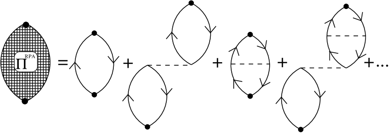
FIG. 5.: Diagrammatic representation of the perturbative expansion for the polarization propagator in the random phase approximation.

We have already noted at the beginning of Section II A that, while for the two-body Green’s function $G^{\text{ph}}$ one can introduce an integral equation, this is not in general possible for the polarization propagator. It becomes possible when one approximates the irreducible vertex function $\Gamma^{13}$ with the direct matrix elements of the interaction. In that case, in an infinite system one gets a simple algebraic equation whose solution, for the polarization propagators in Eq. (2) and the interaction in Eq. (2), is readily found to be

$$\Pi^{\text{ring}}_{\text{X}}(q,\omega)=\frac{\Pi^{(0)}(q,\omega)}{1-\Pi^{(1)\text{d}}_{\text{X}}(q,\omega)\big{/}\Pi^{(0)}(q,\omega)},$$ (82)

where $\Pi^{(1)\text{d}}_{\text{X}}$ represents the first-order direct polarization propagator:

$$\Pi^{(1)\text{d}}_{\text{L};I=0(1)}(q,\omega) = \Pi^{(0)}(q,\omega)4V_{0(\tau)}(q)\Pi^{(0)}(q,\omega),$$ (84)

$$\Pi^{(1)\text{d}}_{\text{T};I=0(1)}(q,\omega) = \Pi^{(0)}(q,\omega)4[V_{\sigma(\sigma\tau)}(q)-V_{t(t\tau)}(q)]\Pi^{(0)}(q,\omega).$$ (85)

The effect of the exchange diagrams is often included through an effective zero-range interaction, calculated by taking the limit $q\to 0$ of the first-order exchange contribution and rewriting it as an effective first-order direct term [33]. Exact calculations, however, show that extrapolating this approximation to finite transferred momenta is not always reliable [6].

A more advanced approximation scheme is given by the continued fraction (CF) expansion [34, 4, 5, 35]. At infinite order the CF expansion exactly corresponds to the summation of the perturbative series, so that it is not any easier to calculate than the exact expression. However, when truncated at finite order, not only does it reproduce the standard perturbative series at the same order, but in addition it yields an estimate for each one of the infinite number of higher-order contributions. Regrettably no general methods are available to predict the convergence of the CF expansion, the only reliable test being to compare the results at successive orders.

On the other hand, one should note that for zero-range forces the first-order CF expansion already gives the exact (albeit trivial) result, making one hope that the short-range nature of the nuclear interactions allows for a fast convergence. Indeed, all available calculations have been performed truncating the CF expansion at first order [4, 5, 27, 28, 14, 23]. Here, as anticipated, we shall test the convergence up to second order.

The CF formalism for the polarization propagator is developed in Ref. [4] for the case of Tamm-Dancoff correlations and extended in Ref. [5] to the full RPA. Instead of following the rather involved formal derivation given there, here we shall briefly sketch a sort of heuristic derivation of the CF expansion.

Let us assume that we want to build a CF-like expansion for the polarization propagator, according to the pattern

$$\Pi^{\text{RPA}}=\frac{\Pi^{(0)}}{\displaystyle 1-A-\frac{B}{\displaystyle 1-C-\frac{D}{\displaystyle 1-...}}}.$$ (86)

We have said that the CF approach at $n$-th order exactly corresponds to the perturbative series at the same order and then it approximates the higher orders. Thus, if we want to approximate the exact RPA propagator at first order in CF (for sake of illustration we drop spin-isospin indices),

$$\Pi^{\text{RPA}}=\sum_{n=0}^{\infty}\Pi^{(n)},$$ (87)

we can rather naturally set

$$\Pi^{(n)}\cong\Pi^{(0)}\left[\frac{\Pi^{(1)}}{\Pi^{(0)}}\right]^{n}.$$ (88)

In Eq. (88) $\Pi^{(1)}\equiv\Pi^{(0)}4V\Pi^{(0)}+\Pi^{(1)\text{ex}}$ is the sum of the direct and exchange first-order terms of RPA — since this yields the correct expression for the direct terms. With the approximation in Eq. (88) the summation is trivial, yielding

$$\Pi^{\text{RPA}}_{\text{CF1}}=\frac{\Pi^{(0)}}{1-\Pi^{(1)}/\Pi^{(0)}}=\frac{\Pi^{(0)}}{1-4V\Pi^{(0)}-\Pi^{(1)\text{ex}}/\Pi^{(0)}}.$$ (89)

We could then add in the denominator of the above expression the exact second-order term, $\Pi^{(2)}$, after subtracting its approximate estimate given by the first-order CF expansion, $[\Pi^{(1)}]^{2}/\Pi^{(0)}$. We would thus obtain

$$\Pi^{\text{RPA}}_{\text{CF2}} = \frac{\Pi^{(0)}}{1-\Pi^{(1)}/\Pi^{(0)}-\{\Pi^{(2)}/\Pi^{(0)}-[\Pi^{(1)}/\Pi^{(0)}]^{2}\}}$$ (90)

$$= \frac{\Pi^{(0)}}{1-4V\Pi^{(0)}-\Pi^{(1)\text{ex}}/\Pi^{(0)}-\{\Pi^{(2)\text{ex}}/\Pi^{(0)}-[\Pi^{(1)\text{ex}}/\Pi^{(0)}]^{2}\}}.$$ (91)

It is easily deduced from Eq. (91) that the third-order term is approximated as $\Pi^{(3)}\cong\Pi^{(1)}\{2\Pi^{(2)}/\Pi^{(0)}-[\Pi^{(1)}/\Pi^{(0)}]^{2}\}$. Then, going ahead in a CF-style expansion we would guess for the exact RPA propagator the following expression:

$$\Pi^{\text{RPA}}=\frac{\Pi^{(0)}}{\displaystyle 1-\Pi^{(1)}/\Pi^{(0)}-\frac{\Pi^{(2)\text{ex}}/\Pi^{(0)}-[\Pi^{(1)\text{ex}}/\Pi^{(0)}]^{2}}{\displaystyle 1-\frac{\Pi^{(3)\text{ex}}/\Pi^{(0)}+[\Pi^{(1)\text{ex}}/\Pi^{(0)}]^{3}-2[\Pi^{(1)\text{ex}}/\Pi^{(0)}][\Pi^{(2)\text{ex}}/\Pi^{(0)}]}{\displaystyle\Pi^{(2)\text{ex}}/\Pi^{(0)}-[\Pi^{(1)\text{ex}}/\Pi^{(0)}]^{2}}-...}}.$$ (92)

This is the expression that one would get from the formalism of Refs. [4, 5] when the expansion up to third order is worked out. Note that we did not assume any specific scheme (either Tamm-Dancoff or RPA) in this heuristic derivation.

Thus, following Eq. (82), we can write

$$\Pi^{\text{RPA}}_{\text{X}}=\frac{\Pi^{(0)}}{\displaystyle 1-\Pi^{(1)\text{d}}_{\text{X}}\big{/}\Pi^{(0)}-\Pi^{(1)\text{ex}}_{\text{X}}\big{/}\Pi^{(0)}-\frac{\Pi^{(2)\text{ex}}_{\text{X}}\big{/}\Pi^{(0)}-\left[\Pi^{(1)\text{ex}}_{\text{X}}\big{/}\Pi^{(0)}\right]^{2}}{\displaystyle 1-...}},$$ (93)

where $\Pi^{(1)\text{d}}_{\text{X}}$ has been defined in Eq. (82). Clearly, a truncation at $n$-th order would require the calculation of the exchange contributions up to that order. Exploiting Eq. (2) these can be cast in the form

$$\Pi^{(n)\text{ex}}_{\text{L};I}(q,\omega) = \text{tr}[\hat{O}^{I}_{\text{L}}\hat{\Pi}^{(n)\text{ex}}(q,\omega)\hat{O}^{I}_{\text{L}}]=\sum_{\alpha_{i}}C^{\alpha_{1}...\alpha_{n}}_{\text{L};I}\Pi^{(n)\text{ex}}_{\alpha_{1}...\alpha_{n}}(q,\omega),$$ (95)

$$\Pi^{(n)\text{ex}}_{\text{T};I}(q,\omega) = \sum_{ij}\Lambda_{ji}\text{tr}[\hat{O}^{I}_{\text{T};i}\hat{\Pi}^{(n)\text{ex}}(q,\omega)\hat{O}^{I}_{\text{T};j}]=\sum_{\alpha_{i}}C^{\alpha_{1}...\alpha_{n}}_{\text{T};I}\Pi^{(n)\text{ex}}_{\alpha_{1}...\alpha_{n}}(q,\omega),$$ (96)

where the indices $\alpha_{i}$ run over all the spin-isospin channels and the spin-isospin factors are absorbed into the coefficients $C^{\alpha_{1}...\alpha_{n}}_{\text{X}}\equiv C^{(\alpha_{1})}_{\text{X}}C^{(\alpha_{2})}_{\text{X}}...C^{(\alpha_{n})}_{\text{X}}$ (see Table I).

$\phantom{\Big{|}}X$	$C^{0}_{X}$	$C^{\tau}_{X}$	$C^{\sigma}_{X}$	$C^{\sigma\tau}_{X}$	$C^{t}_{X}$	$C^{t\tau}_{X}$
$L;I=0$	1	3	3	9	0	0
$L;I=1$	1	-1	3	-3	0	0
$T;I=0$	1	3	-1	-3	-1	-3
$T;I=1$	1	-1	-1	1	-1	1

TABLE I.: The spin-isospin coefficients $C^{\alpha}_{X}$ (see text) in the longitudinal and transverse isoscalar and isovector channels, for the interaction in Eq. (2).

Moreover the “elementary” exchange contribution $\Pi^{(n)\text{ex}}_{\alpha_{1}...\alpha_{n}}$ containing $n$ interaction lines $V_{\alpha_{1}}$…$V_{\alpha_{n}}$, namely

$$\Pi^{(n)\text{ex}}_{\alpha_{1}...\alpha_{n}}(q,\omega) = -i^{n+1}\int\frac{d^{4}K_{1}}{(2\pi)^{4}}\cdot\cdot\cdot\frac{d^{4}K_{n+1}}{(2\pi)^{4}}G^{(0)}(K_{1})G^{(0)}(K_{1}+Q)V_{\alpha_{1}}(\mathchoice{{\hbox{\boldmath$\displaystyle k$}}}{{\hbox{\boldmath$\textstyle k$}}}{{\hbox{\boldmath$\scriptstyle k$}}}{{\hbox{\boldmath$\scriptscriptstyle k$}}}_{1}-\mathchoice{{\hbox{\boldmath$\displaystyle k$}}}{{\hbox{\boldmath$\textstyle k$}}}{{\hbox{\boldmath$\scriptstyle k$}}}{{\hbox{\boldmath$\scriptscriptstyle k$}}}_{2})\cdot\cdot\cdot$$ (98)

$$\qquad\cdot\cdot\cdot V_{\alpha_{n}}(\mathchoice{{\hbox{\boldmath$\displaystyle k$}}}{{\hbox{\boldmath$\textstyle k$}}}{{\hbox{\boldmath$\scriptstyle k$}}}{{\hbox{\boldmath$\scriptscriptstyle k$}}}_{n}-\mathchoice{{\hbox{\boldmath$\displaystyle k$}}}{{\hbox{\boldmath$\textstyle k$}}}{{\hbox{\boldmath$\scriptstyle k$}}}{{\hbox{\boldmath$\scriptscriptstyle k$}}}_{n+1})G^{(0)}(K_{n+1})G^{(0)}(K_{n+1}+Q)$$

$$= (-1)^{n}\int\frac{d\mathchoice{{\hbox{\boldmath$\displaystyle k$}}}{{\hbox{\boldmath$\textstyle k$}}}{{\hbox{\boldmath$\scriptstyle k$}}}{{\hbox{\boldmath$\scriptscriptstyle k$}}}_{1}}{(2\pi)^{3}}\cdot\cdot\cdot\frac{d\mathchoice{{\hbox{\boldmath$\displaystyle k$}}}{{\hbox{\boldmath$\textstyle k$}}}{{\hbox{\boldmath$\scriptstyle k$}}}{{\hbox{\boldmath$\scriptscriptstyle k$}}}_{n+1}}{(2\pi)^{3}}G^{(0)}_{\text{ph}}(\mathchoice{{\hbox{\boldmath$\displaystyle k$}}}{{\hbox{\boldmath$\textstyle k$}}}{{\hbox{\boldmath$\scriptstyle k$}}}{{\hbox{\boldmath$\scriptscriptstyle k$}}}_{1},\mathchoice{{\hbox{\boldmath$\displaystyle q$}}}{{\hbox{\boldmath$\textstyle q$}}}{{\hbox{\boldmath$\scriptstyle q$}}}{{\hbox{\boldmath$\scriptscriptstyle q$}}};\omega)V_{\alpha_{1}}(\mathchoice{{\hbox{\boldmath$\displaystyle k$}}}{{\hbox{\boldmath$\textstyle k$}}}{{\hbox{\boldmath$\scriptstyle k$}}}{{\hbox{\boldmath$\scriptscriptstyle k$}}}_{1}-\mathchoice{{\hbox{\boldmath$\displaystyle k$}}}{{\hbox{\boldmath$\textstyle k$}}}{{\hbox{\boldmath$\scriptstyle k$}}}{{\hbox{\boldmath$\scriptscriptstyle k$}}}_{2})\cdot\cdot\cdot$$ (100)

$$\qquad\cdot\cdot\cdot V_{\alpha_{n}}(\mathchoice{{\hbox{\boldmath$\displaystyle k$}}}{{\hbox{\boldmath$\textstyle k$}}}{{\hbox{\boldmath$\scriptstyle k$}}}{{\hbox{\boldmath$\scriptscriptstyle k$}}}_{n}-\mathchoice{{\hbox{\boldmath$\displaystyle k$}}}{{\hbox{\boldmath$\textstyle k$}}}{{\hbox{\boldmath$\scriptstyle k$}}}{{\hbox{\boldmath$\scriptscriptstyle k$}}}_{n+1})G^{(0)}_{\text{ph}}(\mathchoice{{\hbox{\boldmath$\displaystyle k$}}}{{\hbox{\boldmath$\textstyle k$}}}{{\hbox{\boldmath$\scriptstyle k$}}}{{\hbox{\boldmath$\scriptscriptstyle k$}}}_{n+1},\mathchoice{{\hbox{\boldmath$\displaystyle q$}}}{{\hbox{\boldmath$\textstyle q$}}}{{\hbox{\boldmath$\scriptstyle q$}}}{{\hbox{\boldmath$\scriptscriptstyle q$}}};\omega)$$

have been introduced. With the definition of $G^{(0)}_{\text{ph}}$ given in Eq. (38) and by a suitable change of integration variables one can eliminate all of the $\theta$-functions that contain angular integration variables, leaving a multiple integral with the following general structure:

$$\Pi^{(n)\text{ex}}_{\alpha_{1}...\alpha_{n}}(q,\omega)=(-1)^{n}\int\frac{d\mathchoice{{\hbox{\boldmath$\displaystyle k$}}}{{\hbox{\boldmath$\textstyle k$}}}{{\hbox{\boldmath$\scriptstyle k$}}}{{\hbox{\boldmath$\scriptscriptstyle k$}}}_{1}}{(2\pi)^{3}}\theta(k_{F}-k_{1})\cdot\cdot\cdot\frac{d\mathchoice{{\hbox{\boldmath$\displaystyle k$}}}{{\hbox{\boldmath$\textstyle k$}}}{{\hbox{\boldmath$\scriptstyle k$}}}{{\hbox{\boldmath$\scriptscriptstyle k$}}}_{n+1}}{(2\pi)^{3}}\theta(k_{F}-k_{n+1})$$ (101)

$$\quad\times\Big{[}\frac{1}{\omega-\epsilon_{\mathchoice{{\hbox{\boldmath$\displaystyle k$}}}{{\hbox{\boldmath$\textstyle k$}}}{{\hbox{\boldmath$\scriptstyle k$}}}{{\hbox{\boldmath$\scriptscriptstyle k$}}}_{1}+\mathchoice{{\hbox{\boldmath$\displaystyle q$}}}{{\hbox{\boldmath$\textstyle q$}}}{{\hbox{\boldmath$\scriptstyle q$}}}{{\hbox{\boldmath$\scriptscriptstyle q$}}}}+\epsilon_{\mathchoice{{\hbox{\boldmath$\displaystyle k$}}}{{\hbox{\boldmath$\textstyle k$}}}{{\hbox{\boldmath$\scriptstyle k$}}}{{\hbox{\boldmath$\scriptscriptstyle k$}}}_{1}}+i\eta_{\omega}}V_{\alpha_{1}}(\mathchoice{{\hbox{\boldmath$\displaystyle k$}}}{{\hbox{\boldmath$\textstyle k$}}}{{\hbox{\boldmath$\scriptstyle k$}}}{{\hbox{\boldmath$\scriptscriptstyle k$}}}_{1}-\mathchoice{{\hbox{\boldmath$\displaystyle k$}}}{{\hbox{\boldmath$\textstyle k$}}}{{\hbox{\boldmath$\scriptstyle k$}}}{{\hbox{\boldmath$\scriptscriptstyle k$}}}_{2})\cdot\cdot\cdot V_{\alpha_{n}}(\mathchoice{{\hbox{\boldmath$\displaystyle k$}}}{{\hbox{\boldmath$\textstyle k$}}}{{\hbox{\boldmath$\scriptstyle k$}}}{{\hbox{\boldmath$\scriptscriptstyle k$}}}_{n}-\mathchoice{{\hbox{\boldmath$\displaystyle k$}}}{{\hbox{\boldmath$\textstyle k$}}}{{\hbox{\boldmath$\scriptstyle k$}}}{{\hbox{\boldmath$\scriptscriptstyle k$}}}_{n+1})\frac{1}{\omega-\epsilon_{\mathchoice{{\hbox{\boldmath$\displaystyle k$}}}{{\hbox{\boldmath$\textstyle k$}}}{{\hbox{\boldmath$\scriptstyle k$}}}{{\hbox{\boldmath$\scriptscriptstyle k$}}}_{n+1}+\mathchoice{{\hbox{\boldmath$\displaystyle q$}}}{{\hbox{\boldmath$\textstyle q$}}}{{\hbox{\boldmath$\scriptstyle q$}}}{{\hbox{\boldmath$\scriptscriptstyle q$}}}}+\epsilon_{\mathchoice{{\hbox{\boldmath$\displaystyle k$}}}{{\hbox{\boldmath$\textstyle k$}}}{{\hbox{\boldmath$\scriptstyle k$}}}{{\hbox{\boldmath$\scriptscriptstyle k$}}}_{n+1}}+i\eta_{\omega}}$$ (102)

$$\quad\quad+\sum(\omega\to-\omega)\Big{]}.$$ (103)

In Eq. (103), $\sum(\omega\to-\omega)$ stands for the sum of all the terms generated according to the following rules:

• Take all of the terms obtained by substituting $\omega\to-\omega$ in one energy denominator in the second line of Eq. (103); then add the contribution obtained by performing the same substitution in two energy denominators and so on up to when the replacement $\omega\to-\omega$ has been performed in all the $n+1$ denominators;

• Every time $(\omega-\epsilon_{\mathchoice{{\hbox{\boldmath$\displaystyle k$}}}{{\hbox{\boldmath$\textstyle k$}}}{{\hbox{\boldmath$\scriptstyle k$}}}{{\hbox{\boldmath$\scriptscriptstyle k$}}}_{i}+\mathchoice{{\hbox{\boldmath$\displaystyle q$}}}{{\hbox{\boldmath$\textstyle q$}}}{{\hbox{\boldmath$\scriptstyle q$}}}{{\hbox{\boldmath$\scriptscriptstyle q$}}}}+\epsilon_{\mathchoice{{\hbox{\boldmath$\displaystyle k$}}}{{\hbox{\boldmath$\textstyle k$}}}{{\hbox{\boldmath$\scriptstyle k$}}}{{\hbox{\boldmath$\scriptscriptstyle k$}}}_{i}}+i\eta_{\omega})^{-1}$ is replaced with $(-\omega-\epsilon_{\mathchoice{{\hbox{\boldmath$\displaystyle k$}}}{{\hbox{\boldmath$\textstyle k$}}}{{\hbox{\boldmath$\scriptstyle k$}}}{{\hbox{\boldmath$\scriptscriptstyle k$}}}_{i}+\mathchoice{{\hbox{\boldmath$\displaystyle q$}}}{{\hbox{\boldmath$\textstyle q$}}}{{\hbox{\boldmath$\scriptstyle q$}}}{{\hbox{\boldmath$\scriptscriptstyle q$}}}}+\epsilon_{\mathchoice{{\hbox{\boldmath$\displaystyle k$}}}{{\hbox{\boldmath$\textstyle k$}}}{{\hbox{\boldmath$\scriptstyle k$}}}{{\hbox{\boldmath$\scriptscriptstyle k$}}}_{i}}-i\eta_{\omega})^{-1}$ then replace $\mathchoice{{\hbox{\boldmath$\displaystyle k$}}}{{\hbox{\boldmath$\textstyle k$}}}{{\hbox{\boldmath$\scriptstyle k$}}}{{\hbox{\boldmath$\scriptscriptstyle k$}}}_{i}$ with $-\mathchoice{{\hbox{\boldmath$\displaystyle k$}}}{{\hbox{\boldmath$\textstyle k$}}}{{\hbox{\boldmath$\scriptstyle k$}}}{{\hbox{\boldmath$\scriptscriptstyle k$}}}_{i}-\mathchoice{{\hbox{\boldmath$\displaystyle q$}}}{{\hbox{\boldmath$\textstyle q$}}}{{\hbox{\boldmath$\scriptstyle q$}}}{{\hbox{\boldmath$\scriptscriptstyle q$}}}$ in the potential.

The number of integrations can be reduced by noticing that the azimuthal angles are contained only in the potential functions $V_{\alpha_{i}}$. For typical potentials this integration can be done analytically, hence it is convenient to introduce a new function representing the azimuthal integral of the potential. To this end, define the new variables:

$$|\mathchoice{{\hbox{\boldmath$\displaystyle k$}}}{{\hbox{\boldmath$\textstyle k$}}}{{\hbox{\boldmath$\scriptstyle k$}}}{{\hbox{\boldmath$\scriptscriptstyle k$}}}-\mathchoice{{\hbox{\boldmath$\displaystyle k$}}}{{\hbox{\boldmath$\textstyle k$}}}{{\hbox{\boldmath$\scriptstyle k$}}}{{\hbox{\boldmath$\scriptscriptstyle k$}}}^{\prime}| = \sqrt{k^{2}+{k^{\prime}}^{2}-2kk^{\prime}[\cos\theta\,\cos\theta^{\prime}+\sin\theta\,\sin\theta^{\prime}\,\cos(\varphi-\varphi^{\prime})]}$$ (104)

$$= \sqrt{k^{2}+{k^{\prime}}^{2}-2[yy^{\prime}+\sqrt{k^{2}-y^{2}}\sqrt{{k^{\prime}}^{2}-{y^{\prime}}^{2}}\cos(\varphi-\varphi^{\prime})]}$$ (105)

$$= \sqrt{x+x^{\prime}-2\sqrt{x}\sqrt{x^{\prime}}\cos(\varphi-\varphi^{\prime})+(y-y^{\prime})^{2}},$$ (106)

where $y\equiv k\,\cos\theta$ and $x\equiv k^{2}-y^{2}$. Then, one can introduce

$$W_{\alpha}(x,y;x^{\prime},y^{\prime})=\int_{0}^{2\pi}\frac{d\varphi}{2\pi}V_{\alpha}(\mathchoice{{\hbox{\boldmath$\displaystyle k$}}}{{\hbox{\boldmath$\textstyle k$}}}{{\hbox{\boldmath$\scriptstyle k$}}}{{\hbox{\boldmath$\scriptscriptstyle k$}}}-\mathchoice{{\hbox{\boldmath$\displaystyle k$}}}{{\hbox{\boldmath$\textstyle k$}}}{{\hbox{\boldmath$\scriptstyle k$}}}{{\hbox{\boldmath$\scriptscriptstyle k$}}}^{\prime})=W_{\alpha}(x^{\prime},y^{\prime};x,y)$$ (107)

and rewrite Eq. (103) as

$$\Pi^{(n)\text{ex}}_{\alpha_{1}...\alpha_{n}}(q,\omega) = (-1)^{n}\left(\frac{m_{N}}{q}\right)^{n+1}\left(\frac{k_{F}}{2\pi}\right)^{2n+2}\int_{-1}^{1}dy_{1}\frac{1}{2}\int_{0}^{1-y_{1}^{2}}dx_{1}\cdot\cdot\cdot\int_{-1}^{1}dy_{n+1}\frac{1}{2}\int_{0}^{1-y_{n+1}^{2}}dx_{n+1}$$ (110)

$$\times\frac{1}{\psi-y_{1}+i\eta_{\omega}}W_{\alpha_{1}}(x_{1},y_{1};x_{2},y_{2})\cdot\cdot\cdot W_{\alpha_{n}}(x_{n},y_{n};x_{n+1},y_{n+1})\frac{1}{\psi-y_{n+1}+i\eta_{\omega}}$$

$$+\sum(\omega\to-\omega).$$

For $n=1$ one has

$$\Pi^{(1)\text{ex}}_{\alpha}(q,\omega) = -\left(\frac{m_{N}}{q}\right)^{2}\frac{k_{F}^{4}}{(2\pi)^{4}}\int_{-1}^{1}dy\frac{1}{2}\int_{0}^{1-y^{2}}dx\int_{-1}^{1}dy^{\prime}\frac{1}{2}\int_{0}^{1-{y^{\prime}}^{2}}dx^{\prime}$$ (113)

$$\times\frac{1}{\psi-y+i\eta_{\omega}}W_{\alpha}(x,y;x^{\prime},y^{\prime})\frac{1}{\psi-y^{\prime}+i\eta_{\omega}}$$

$$+\sum(\omega\to-\omega)$$

$$= -\left(\frac{m_{N}}{q}\right)^{2}\frac{k_{F}^{4}}{(2\pi)^{4}}\left[{\cal Q}_{\alpha}^{(1)}(0,\psi)-{\cal Q}_{\alpha}^{(1)}(\bar{q},\psi)+{\cal Q}_{\alpha}^{(1)}(0,\psi+\bar{q})-{\cal Q}_{\alpha}^{(1)}(-\bar{q},\psi+\bar{q})\right],$$ (114)

where

$${\cal Q}_{\alpha}^{(1)}(\bar{q},\psi)=2\int_{-1}^{1}dy\frac{1}{\psi-y+i\eta_{\omega}}\int_{-1}^{1}dy^{\prime}\,{W_{\alpha}}^{\prime\prime}(y,y^{\prime};\bar{q})\frac{1}{y-y^{\prime}+\bar{q}}$$ (116)

and

$$W^{\prime\prime}_{\alpha}(y,y^{\prime};\bar{q})=\frac{1}{2}\int_{0}^{1-y^{2}}dx\,\frac{1}{2}\int_{0}^{1-{y^{\prime}}^{2}}dx^{\prime}\,W_{\alpha}(x,y+\bar{q};x^{\prime},y^{\prime}).$$ (117)

Note that in getting to Eq. (116) use has been made of the Poincaré–Bertrand theorem [36]. For the potential in Eq. (* ‣ II A) $W^{\prime\prime}_{\alpha}$ can be calculated analytically (see Appendix D), so that the calculation of the first-order exchange contribution to the polarization propagator is reduced to the numerical evaluation of two-dimensional integrals for the real part and of one-dimensional integrals for the imaginary part.

For $n=2$ one has

$$\Pi^{(2)\text{ex}}_{\alpha\alpha^{\prime}}(q,\omega)=\left(\frac{m_{N}}{q}\right)^{3}\frac{k_{F}^{6}}{(2\pi)^{6}}\int_{-1}^{1}dy_{1}\frac{1}{2}\int_{0}^{1-y_{1}^{2}}dx_{1}\int_{-1}^{1}dy_{2}\frac{1}{2}\int_{0}^{1-y_{2}^{2}}dx_{2}\int_{-1}^{1}dy_{3}\frac{1}{2}\int_{0}^{1-y_{3}^{2}}dx_{3}$$ (118)

$$\phantom{\Pi^{(2)\text{ex}}_{\alpha\alpha^{\prime}}(q,\omega)=}\times\frac{1}{\psi-y_{1}+i\eta_{\omega}}W_{\alpha}(x_{1},y_{1};x_{2},y_{2})\frac{1}{\psi-y_{2}+i\eta_{\omega}}W_{\alpha}(x_{2},y_{2};x_{3},y_{3})\frac{1}{\psi-y_{3}+i\eta_{\omega}}$$ (119)

$$\phantom{\Pi^{(2)\text{ex}}_{\alpha\alpha^{\prime}}(q,\omega)=}+\sum(\omega\to-\omega)$$ (120)

$$\phantom{\Pi^{(2)\text{ex}}_{\alpha\alpha^{\prime}}(q,\omega)}=\left(\frac{m_{N}}{q}\right)^{3}\frac{k_{F}^{6}}{(2\pi)^{6}}\left[{\cal Q}_{\alpha\alpha^{\prime}}^{(2)}(0,0;\psi)-{\cal Q}_{\alpha\alpha^{\prime}}^{(2)}(0,\bar{q};\psi)-{\cal Q}_{\alpha\alpha^{\prime}}^{(2)}(\bar{q},0;\psi)+{\cal Q}_{\alpha\alpha^{\prime}}^{(2)}(\bar{q},\bar{q};\psi)\right.$$ (121)

$$\qquad\left.-{\cal Q}_{\alpha\alpha^{\prime}}^{(2)}(0,0;\psi+\bar{q})+{\cal Q}_{\alpha\alpha^{\prime}}^{(2)}(0,-\bar{q};\psi+\bar{q})+{\cal Q}_{\alpha\alpha^{\prime}}^{(2)}(-\bar{q},0;\psi+\bar{q})-{\cal Q}_{\alpha\alpha^{\prime}}^{(2)}(-\bar{q},-\bar{q};\psi+\bar{q})\right],$$ (122)

(123)

where

$${\cal Q}_{\alpha\alpha^{\prime}}^{(2)}(\bar{q}_{1},\bar{q}_{2};\psi)=\int_{-1}^{1}dy\frac{1}{2}\int_{0}^{1-y^{2}}dx\,{\cal G}_{\alpha}(x,y+\bar{q}_{1};\psi+\bar{q}_{1})\frac{1}{\psi-y+i\eta_{\omega}}{\cal G}_{\alpha^{\prime}}(x,y+\bar{q}_{2};\psi+\bar{q}_{2})$$ (124)

and

$${\cal G}_{\alpha}(x,y;\psi) = \int_{-1}^{1}dy^{\prime}\frac{1}{\psi-y^{\prime}+i\eta_{\omega}}W^{\prime}_{\alpha}(x,y;y^{\prime}),$$ (126)

$$W^{\prime}_{\alpha}(x,y;y^{\prime}) = \frac{1}{2}\int_{0}^{1-{y^{\prime}}^{2}}dx^{\prime}\,W_{\alpha}(x,y;x^{\prime},y^{\prime}).$$ (127)

For the potential in Eq. (* ‣ II A) $W^{\prime}_{\alpha}$ can be calculated analytically (see Appendix D) and one is left with the numerical integration of Eqs. (124) and (126), so that the calculation of the second-order exchange contribution to the polarization propagator is effectively reduced to the numerical evaluation of at most three-dimensional integrals. Higher orders add a numerical two-dimensional integration for each additional interaction line, since, for a potential of the form in Eq. (* ‣ II A), only the azimuthal integration can be performed analytically for the interaction lines that do not close on the external vertices.

Finally we recall that the nucleon propagators can be dressed by the HF field, as explained in Section II D, by replacing $\psi\to\psi^{*}$ and $m_{N}\to m_{N}^{*}$, where $\psi^{*}$ and $m_{N}^{*}$ have been defined in Eqs. (72) and (77), multiplying by the appropriate power of the normalization factor $1+\omega/m_{N}+\Delta^{(1)}/m_{N}$ when relativistic kinematics are employed (see Eqs. (3) and (81)).

F Effective particle-hole interaction

In order to assess the contributions to the nuclear responses arising from the various approximation schemes introduced so far and to show typical results, first of all we have to choose an effective interaction. This choice can be rather delicate as it may introduce uncontrolled uncertainties in the calculation. Here, however, we are not interested so much in comparisons with data, but rather with setting up working many-body schemes. For this purpose, we shall use the $G$-matrix based on the Bonn potential of Ref. [25], adapted to the quasielastic regime as in Ref. [37]. Although the attraction provided in the scalar-isoscalar channel by this interaction is definitely too strong [37], it will serve our illustrative needs.

Two approaches to determine the effective ph interaction in the nuclear medium appear to be possible: one can either directly fix an effective potential by fitting some phenomenological properties or start with a bare nucleon-nucleon interaction and calculate the related $G$-matrix. Parameterizations of the ph interaction based upon the first procedure are generally only available at very low momentum transfers (in terms of Migdal-Landau parameters), and since we are probing relatively high momenta, we have resorted to using a $G$-matrix. We have chosen the one of Ref. [25], that, in our view, has the following appealing features: it is based upon a realistic boson-exchange potential; it accounts for the density dependence; and it includes (nonlocal) exchange contributions in the effective interaction, which are conveniently parameterized in terms of Yukawa functions.

A feature related to the effective inclusion of antisymmetrization effects is particularly interesting in order to test a specific widely employed approximation scheme, the so-called ring approximation, in which the exchange diagrams of the RPA series are dropped and their effect mimicked by adding to the direct interaction matrix elements an effective exchange contribution (see, e. g., Ref. [33]). Indeed, below we shall compare calculations employing the fully antisymmetrized formalism developed in the previous subsections using the direct part of the $G$-matrix, to those employing the ring approximation using the antisymmetrized effective interaction.

To facilitate the comparison with the original parameterization of Ref. [25], the potential is given here using the standard representation of Eq. (2) in spin and isospin (no spin-orbit contribution will be considered in the following), but employing different symbols for the momentum space potentials (and adding the tensor contributions in the exchange channel):

$$V(\mathchoice{{\hbox{\boldmath$\displaystyle k$}}}{{\hbox{\boldmath$\textstyle k$}}}{{\hbox{\boldmath$\scriptstyle k$}}}{{\hbox{\boldmath$\scriptscriptstyle k$}}}_{f},\mathchoice{{\hbox{\boldmath$\displaystyle k$}}}{{\hbox{\boldmath$\textstyle k$}}}{{\hbox{\boldmath$\scriptstyle k$}}}{{\hbox{\boldmath$\scriptscriptstyle k$}}}_{i};k_{F}) = F+F^{\prime}\mathchoice{{\hbox{\boldmath$\displaystyle\tau$}}}{{\hbox{\boldmath$\textstyle\tau$}}}{{\hbox{\boldmath$\scriptstyle\tau$}}}{{\hbox{\boldmath$\scriptscriptstyle\tau$}}}_{1}\cdot\mathchoice{{\hbox{\boldmath$\displaystyle\tau$}}}{{\hbox{\boldmath$\textstyle\tau$}}}{{\hbox{\boldmath$\scriptstyle\tau$}}}{{\hbox{\boldmath$\scriptscriptstyle\tau$}}}_{2}+G\mathchoice{{\hbox{\boldmath$\displaystyle\sigma$}}}{{\hbox{\boldmath$\textstyle\sigma$}}}{{\hbox{\boldmath$\scriptstyle\sigma$}}}{{\hbox{\boldmath$\scriptscriptstyle\sigma$}}}_{1}\cdot\mathchoice{{\hbox{\boldmath$\displaystyle\sigma$}}}{{\hbox{\boldmath$\textstyle\sigma$}}}{{\hbox{\boldmath$\scriptstyle\sigma$}}}{{\hbox{\boldmath$\scriptscriptstyle\sigma$}}}_{2}+G^{\prime}\mathchoice{{\hbox{\boldmath$\displaystyle\sigma$}}}{{\hbox{\boldmath$\textstyle\sigma$}}}{{\hbox{\boldmath$\scriptstyle\sigma$}}}{{\hbox{\boldmath$\scriptscriptstyle\sigma$}}}_{1}\cdot\mathchoice{{\hbox{\boldmath$\displaystyle\sigma$}}}{{\hbox{\boldmath$\textstyle\sigma$}}}{{\hbox{\boldmath$\scriptstyle\sigma$}}}{{\hbox{\boldmath$\scriptscriptstyle\sigma$}}}_{2}\ \mathchoice{{\hbox{\boldmath$\displaystyle\tau$}}}{{\hbox{\boldmath$\textstyle\tau$}}}{{\hbox{\boldmath$\scriptstyle\tau$}}}{{\hbox{\boldmath$\scriptscriptstyle\tau$}}}_{1}\cdot\mathchoice{{\hbox{\boldmath$\displaystyle\tau$}}}{{\hbox{\boldmath$\textstyle\tau$}}}{{\hbox{\boldmath$\scriptstyle\tau$}}}{{\hbox{\boldmath$\scriptscriptstyle\tau$}}}_{2}$$ (129)

$$+TS_{12}(\hat{\mathchoice{{\hbox{\boldmath$\displaystyle q$}}}{{\hbox{\boldmath$\textstyle q$}}}{{\hbox{\boldmath$\scriptstyle q$}}}{{\hbox{\boldmath$\scriptscriptstyle q$}}}})+T^{\prime}S_{12}(\hat{\mathchoice{{\hbox{\boldmath$\displaystyle q$}}}{{\hbox{\boldmath$\textstyle q$}}}{{\hbox{\boldmath$\scriptstyle q$}}}{{\hbox{\boldmath$\scriptscriptstyle q$}}}})\mathchoice{{\hbox{\boldmath$\displaystyle\tau$}}}{{\hbox{\boldmath$\textstyle\tau$}}}{{\hbox{\boldmath$\scriptstyle\tau$}}}{{\hbox{\boldmath$\scriptscriptstyle\tau$}}}_{1}\cdot\mathchoice{{\hbox{\boldmath$\displaystyle\tau$}}}{{\hbox{\boldmath$\textstyle\tau$}}}{{\hbox{\boldmath$\scriptstyle\tau$}}}{{\hbox{\boldmath$\scriptscriptstyle\tau$}}}_{2}+HS_{12}(\hat{\mathchoice{{\hbox{\boldmath$\displaystyle Q$}}}{{\hbox{\boldmath$\textstyle Q$}}}{{\hbox{\boldmath$\scriptstyle Q$}}}{{\hbox{\boldmath$\scriptscriptstyle Q$}}}})+H^{\prime}S_{12}(\hat{\mathchoice{{\hbox{\boldmath$\displaystyle Q$}}}{{\hbox{\boldmath$\textstyle Q$}}}{{\hbox{\boldmath$\scriptstyle Q$}}}{{\hbox{\boldmath$\scriptscriptstyle Q$}}}})\mathchoice{{\hbox{\boldmath$\displaystyle\tau$}}}{{\hbox{\boldmath$\textstyle\tau$}}}{{\hbox{\boldmath$\scriptstyle\tau$}}}{{\hbox{\boldmath$\scriptscriptstyle\tau$}}}_{1}\cdot\mathchoice{{\hbox{\boldmath$\displaystyle\tau$}}}{{\hbox{\boldmath$\textstyle\tau$}}}{{\hbox{\boldmath$\scriptstyle\tau$}}}{{\hbox{\boldmath$\scriptscriptstyle\tau$}}}_{2}\ ,$$

where $\mathchoice{{\hbox{\boldmath$\displaystyle q$}}}{{\hbox{\boldmath$\textstyle q$}}}{{\hbox{\boldmath$\scriptstyle q$}}}{{\hbox{\boldmath$\scriptscriptstyle q$}}}=\mathchoice{{\hbox{\boldmath$\displaystyle k$}}}{{\hbox{\boldmath$\textstyle k$}}}{{\hbox{\boldmath$\scriptstyle k$}}}{{\hbox{\boldmath$\scriptscriptstyle k$}}}_{i}-\mathchoice{{\hbox{\boldmath$\displaystyle k$}}}{{\hbox{\boldmath$\textstyle k$}}}{{\hbox{\boldmath$\scriptstyle k$}}}{{\hbox{\boldmath$\scriptscriptstyle k$}}}_{f}$, $\mathchoice{{\hbox{\boldmath$\displaystyle Q$}}}{{\hbox{\boldmath$\textstyle Q$}}}{{\hbox{\boldmath$\scriptstyle Q$}}}{{\hbox{\boldmath$\scriptscriptstyle Q$}}}=\mathchoice{{\hbox{\boldmath$\displaystyle k$}}}{{\hbox{\boldmath$\textstyle k$}}}{{\hbox{\boldmath$\scriptstyle k$}}}{{\hbox{\boldmath$\scriptscriptstyle k$}}}_{i}+\mathchoice{{\hbox{\boldmath$\displaystyle k$}}}{{\hbox{\boldmath$\textstyle k$}}}{{\hbox{\boldmath$\scriptstyle k$}}}{{\hbox{\boldmath$\scriptscriptstyle k$}}}_{f}$ ($\mathchoice{{\hbox{\boldmath$\displaystyle k$}}}{{\hbox{\boldmath$\textstyle k$}}}{{\hbox{\boldmath$\scriptstyle k$}}}{{\hbox{\boldmath$\scriptscriptstyle k$}}}_{i}$, $\mathchoice{{\hbox{\boldmath$\displaystyle k$}}}{{\hbox{\boldmath$\textstyle k$}}}{{\hbox{\boldmath$\scriptstyle k$}}}{{\hbox{\boldmath$\scriptscriptstyle k$}}}_{f}$ being the relative momenta in the initial and final states, respectively) and the coefficients are density and momentum dependent.

Before utilizing the interaction of Ref. [25] in a calculation of quasielastic responses, a few issues have to be addressed [37].

a) The density dependence of the $G$-matrix is given in terms of density-dependent coupling constants, which is not very useful for applications to finite nuclei. Furthermore, the parameterization is fitted for 0.95 fm${}^{-1}<k_{F}<$ 1.36 fm^-1, which spans a range of densities down to roughly 1/3 of the central density. Extrapolation of this parameterization to lower densities (which is crucial for application to hadron scattering) gives unreasonable results. Thus, we have chosen to employ a linear $\rho$-dependence ($V=V^{\text{ex}}+V^{\rho}\rho$), which is considered a reasonable choice (see, e. g., Ref. [38]). In Fig. 7 one can see a comparison of the two parameterizations for the $k_{F}$-dependence of the effective interaction. It should be noted that most of the contribution to the quasielastic responses comes from densities where the two descriptions differ by only a few percent.

FIG. 6.: Effective interaction in the non-tensor channels as a function of $k_{F}$ at $q=0$; linear (solid) and from Ref. [25] (dashed) density dependence.

FIG. 7.: (a) Direct and exchange ph matrix elements; (b) direct pp matrix element.

FIG. 8.: Effective ph interaction in the non-tensor channels as a function of $q$ at $k_{F}=1.36$ (solid), 1.25 (dashed), 1.10 (dot-dashed) and 0.95 fm^-1 (dotted).

FIG. 9.: As in Fig. 9, but for the tensor channels; $T$ and $T^{\prime}$ do not depend on the density.

b) In order to obtain a local interaction at a fixed density, one can use the relation between $q$, $Q$ and $k_{i}$, i. e., $Q=\sqrt{4k_{i}^{2}-q^{2}}$ and take for $k_{i}$ a suitably chosen average value, $\langle k_{i}\rangle$; then, the only independent momentum is $q$. The authors of Ref. [25] were interested in a potential for low excitation energy nuclear structure calculations and hence they assumed that the two nucleons in the initial state lie on the Fermi surface and so averaged over the relative angle, getting $\langle k_{i}\rangle\approx 0.7k_{F}$. Clearly, in this case one has the constraint $0<q\lesssim 1.4k_{F}$. On the other hand, we are interested in the ph interaction in the quasielastic region where one nucleon in the initial state is below the Fermi sea, while the other can be well above it. A look at Fig. 7 shows that $\mathchoice{{\hbox{\boldmath$\displaystyle k$}}}{{\hbox{\boldmath$\textstyle k$}}}{{\hbox{\boldmath$\scriptstyle k$}}}{{\hbox{\boldmath$\scriptscriptstyle k$}}}_{i}$ is defined in terms of the particle and hole momenta as $\mathchoice{{\hbox{\boldmath$\displaystyle k$}}}{{\hbox{\boldmath$\textstyle k$}}}{{\hbox{\boldmath$\scriptstyle k$}}}{{\hbox{\boldmath$\scriptscriptstyle k$}}}_{i}=(\mathchoice{{\hbox{\boldmath$\displaystyle p$}}}{{\hbox{\boldmath$\textstyle p$}}}{{\hbox{\boldmath$\scriptstyle p$}}}{{\hbox{\boldmath$\scriptscriptstyle p$}}}-\mathchoice{{\hbox{\boldmath$\displaystyle h$}}}{{\hbox{\boldmath$\textstyle h$}}}{{\hbox{\boldmath$\scriptstyle h$}}}{{\hbox{\boldmath$\scriptscriptstyle h$}}}^{\prime})/2=(\mathchoice{{\hbox{\boldmath$\displaystyle h$}}}{{\hbox{\boldmath$\textstyle h$}}}{{\hbox{\boldmath$\scriptstyle h$}}}{{\hbox{\boldmath$\scriptscriptstyle h$}}}-\mathchoice{{\hbox{\boldmath$\displaystyle h$}}}{{\hbox{\boldmath$\textstyle h$}}}{{\hbox{\boldmath$\scriptstyle h$}}}{{\hbox{\boldmath$\scriptscriptstyle h$}}}^{\prime}+\mathchoice{{\hbox{\boldmath$\displaystyle q$}}}{{\hbox{\boldmath$\textstyle q$}}}{{\hbox{\boldmath$\scriptstyle q$}}}{{\hbox{\boldmath$\scriptscriptstyle q$}}})/2$. Thus, at fixed $\textstyle q$ one should average $k_{i}$ over $\textstyle h$ and $\mathchoice{{\hbox{\boldmath$\displaystyle h$}}}{{\hbox{\boldmath$\textstyle h$}}}{{\hbox{\boldmath$\scriptstyle h$}}}{{\hbox{\boldmath$\scriptscriptstyle h$}}}^{\prime}$, getting $\langle k_{i}\rangle\approx\sqrt{6k_{F}^{2}/5+q^{2}}/2$. Now $k_{i}$ grows with $q$, so that there are no longer constraints on $q$ and the exchange momentum turns out to be constant, $Q=\sqrt{6/5}k_{F}$. In Fig. 9 one can see the resulting interaction in the non-tensor channels.

c) The tensor channels are simpler, since in the parameterization of Ref. [25] there is no explicit density dependence (Fig. 9). The coefficients of the exchange tensor operator, $H$ and $H^{\prime}$, display a very mild density dependence induced by $Q$, which is completely negligible. The only drawback concerns the treatment of $S_{12}(\mathchoice{{\hbox{\boldmath$\displaystyle Q$}}}{{\hbox{\boldmath$\textstyle Q$}}}{{\hbox{\boldmath$\scriptstyle Q$}}}{{\hbox{\boldmath$\scriptscriptstyle Q$}}})$: assuming that $\textstyle q$ and $\textstyle Q$ are orthogonal, with some algebra one can show that $S_{12}(\hat{\mathchoice{{\hbox{\boldmath$\displaystyle Q$}}}{{\hbox{\boldmath$\textstyle Q$}}}{{\hbox{\boldmath$\scriptstyle Q$}}}{{\hbox{\boldmath$\scriptscriptstyle Q$}}}})=-S_{12}(\hat{\mathchoice{{\hbox{\boldmath$\displaystyle q$}}}{{\hbox{\boldmath$\textstyle q$}}}{{\hbox{\boldmath$\scriptstyle q$}}}{{\hbox{\boldmath$\scriptscriptstyle q$}}}})/2$.

G Testing the model

First of all we have to choose the Fermi momentum. Of course, one could easily perform a local density calculation to achieve a better description of finite nuclei. Here, for sake of illustration, we prefer to use the pure Fermi gas. The choice of $k_{F}$ can be made in several ways — here we shall choose an average value according to the formula (see, e. g., [39])

$$\bar{k}_{F}=\frac{1}{A}\int d\mathchoice{{\hbox{\boldmath$\displaystyle r$}}}{{\hbox{\boldmath$\textstyle r$}}}{{\hbox{\boldmath$\scriptstyle r$}}}{{\hbox{\boldmath$\scriptscriptstyle r$}}}k_{F}(r)\rho(r),$$ (130)

where $\rho(r)$ is the empirical Fermi density distribution normalized to the number of nucleons and $k_{F}(r)=[(3\pi/2)\rho(r)]^{1/3}$. For ¹²C one gets $\bar{k}_{F}\approx 195$ MeV/c and this is the value used in the calculations that follow.

Let us start with the HF response. In Fig. 10 we display the HF response of ¹²C at $q=300$, 500 and 1000 MeV/c. As anticipated, Eq. (79) turns out to be a good approximation to the exact expression (54) (except on the borders of the response region, where the Fermi gas is anyway unrealistic). The HF correlations widen the response region and quench and harden the position of the quasielastic peak, as is well known. Note however that the short-range correlations, which are embodied in the effective interaction based on a $G$-matrix, reduce the amount of hardening that is observed in calculations based on the bare Bonn potential [14]. Note also that the same level of accuracy is obtained using either non-relativistic or relativistic kinematics.

FIG. 10.: Fermi gas responses for $k_{F}=195$ MeV/c at $q=300$, 500 and 1000 MeV/c: Free (dotted), exact HF (solid) and HF approximated according to the prescription of Section II D (dashed). The ph interaction is the $G$-matrix discussed in the text; the kinematics are relativistic.

FIG. 11.: Fermi gas longitudinal responses for $k_{F}=195$ MeV/c at $q=300$ MeV/c, with a spin-spin one-boson-exchange interaction, for various values of the coupling constant and of the boson mass: Free response (dotted), RPA with the first-order CF expansion (dashed) and RPA with the second-order CF expansion (solid). Note that in the left and middle panels the dashed and solid lines are indistinguishable. The kinematics are non-relativistic.

FIG. 12.: Modulus of the longitudinal polarization propagator for $k_{F}=195$ MeV/c at $q=300$ MeV/c, with a spin-spin one-boson-exchange interaction, for various values of the coupling constant and of the boson mass: First-order, $\Pi^{\text{(1)}}$ (dotted); exact second-order, $\Pi^{\text{(2)}}$ (dashed); CF approximation to second order, $\Pi^{\text{(2)appr}}={\Pi^{\text{(1)}}}^{2}/\Pi^{\text{(0)}}$ (solid).

Before discussing the RPA results, we would like to test the convergence of the CF expansion. For this purpose, in Fig. 12 we compare the longitudinal RPA responses at first and second order in the CF expansion using a model one-boson-exchange interaction, $V_{\sigma}(k)=\mathchoice{{\hbox{\boldmath$\displaystyle\sigma$}}}{{\hbox{\boldmath$\textstyle\sigma$}}}{{\hbox{\boldmath$\scriptstyle\sigma$}}}{{\hbox{\boldmath$\scriptscriptstyle\sigma$}}}_{1}\cdot\mathchoice{{\hbox{\boldmath$\displaystyle\sigma$}}}{{\hbox{\boldmath$\textstyle\sigma$}}}{{\hbox{\boldmath$\scriptstyle\sigma$}}}{{\hbox{\boldmath$\scriptscriptstyle\sigma$}}}_{2}g[m^{2}/(m^{2}+k^{2})]$ (the spin operators having the purpose of killing the direct (ring) contribution). For values of the coupling constant $g$ and of the boson mass $m$ typical of realistic nucleon-nucleon potentials one finds that the first- and second-order results match at the level of a few percent (in the left and middle panels of Fig. 12, the solid and dashed curves are actually indistinguishable). One has to go to very low boson masses (a few MeV) and, consequently to very high values of $g$ in order to find some discrepancies. To understand these results better, in Fig. 12 we display the modulus of the polarization propagator at first order, $\Pi^{(1)}$ (dotted), at second order, $\Pi^{(2)}$ (dashed) and the approximation to $\Pi^{(2)}$ generated by the first-order CF expansion (see Section II E), $\Pi^{(2)\text{appr}}\equiv{\Pi^{(1)}}^{2}/\Pi^{(0)}$ (solid). From inspection of the curves, it is clear that the first important element to guarantee good convergence is the range of the interaction. Indeed, for $m=800$ MeV (short-range), $\Pi^{(2)}$ and $\Pi^{(2)\text{appr}}$ practically coincide independent of the strength of the interaction. This, of course, should be expected, since for zero-range interactions the first-order CF expansion gives the exact result. For masses of the order of the pion mass one starts finding discrepancies between $\Pi^{(2)}$ and $\Pi^{(2)\text{appr}}$. However, for realistic values of the interaction strength the second-order contribution turns out to be one order of magnitude smaller than the first-order one, and thus these discrepancies have little effect on the full response functions (Fig. 12).

To understand these results it may be useful to compare the strength of the interactions employed here to that of one-pion-exchange, $g_{\pi}m_{\pi}^{2}\equiv f_{\pi}^{2}/3\cong 0.33$ (in natural units). With the same units, the cases with $m=100$ MeV correspond to $g\,m^{2}=0.26$ and 0.65; those with $m=800$ MeV to $g\,m^{2}=16.7$ and 41.7; for $m=1$ and 10 MeV one has $g\,m^{2}=1.3$ and 0.65, respectively.

To summarize, from the left and middle panels of Fig. 12 one can understand that the validity of the CF expansion originates from the interplay between range and strength of the interaction. For short-range potentials where the conventional perturbative expansion may not converge, the CF technique yields a good approximation for the propagators at all orders; for long-range (on the nuclear scale) forces, the CF approximation is less accurate, but the relative weakness of the interaction already guarantees the convergence of the conventional perturbative expansion. One has to go to unreasonably low masses to find a situation where the interaction range is very long and $\Pi^{(1)}$ and $\Pi^{(2)}$ are of the same order (right panels in Fig. 12).

FIG. 13.: Fermi gas longitudinal responses for $k_{F}=195$ MeV/c at $q=300$, 500 and 1000 MeV/c, with the $G$-matrix discussed in the text: Free response (dotted), RPA (dashed) and BHF-RPA (solid). The kinematics are relativistic.

FIG. 14.: The same as in Fig. 14, but for the transverse channel.

We can thus conclude that the calculations of nuclear response functions in the antisymmetrized RPA performed at first order in the CF expansion are indeed quite accurate. The same conclusion is also supported by calculations with a realistic effective interaction — such as the $G$-matrix parameterization discussed above — and including HF and relativistic kinematical effects. In fact, in Fig. 14 we show the RPA and BHF-RPA longitudinal responses of ¹²C at $q=300$, 500 and 1000 MeV/c, using the full $G$-matrix introduced at the beginning of this section. Also for the full interaction, the discrepancies between the first- and second-order CF responses are too small to be displayed. They are at the level of fractions of percent everywhere, except for the case of the isoscalar channel at 300 MeV/c, where they rise to a few percent due to the closeness of a singularity in the propagator induced by the strongly attractive interaction. Indeed, as already mentioned, the scalar-isoscalar channel is (too) attractive and softens the quasielastic peak; the scalar-isovector one is repulsive and gives rise to a hardening. The effect of the HF correlations is the same as in the discussion of Fig. 10. In Fig. 14 the transverse response is displayed for the same conditions.

Finally, it is interesting and important to test the validity of the ring approximation — where exchange diagrams are not included — since this approximation has been widely used in the literature because of its simplicity. In this scheme, the effect of antisymmetrization is simulated by adding to the direct interaction matrix elements an effective exchange contribution (see, e. g., Ref. [33]). For details see also Ref. [37], where a prescription to determine the effective exchange momentum designed for use in the quasifree region has been given.

FIG. 15.: Fermi gas responses for $k_{F}=195$ MeV/c at $q=500$ MeV/c, with the $G$-matrix parameterization discussed in the text: Free response (dotted), ring approximation (dashed) and RPA (solid). The kinematics are relativistic.

In Fig. 15 we display the ring and RPA responses of ¹²C at $q=500$ MeV/c, using the $G$-matrix parameterization. It is apparent that the only channel where the ring approximation works reasonably well is the spin-isovector one, which, incidentally, is the dominant one in ($e$,$e^{\prime}$) magnetic scattering; it is less accurate in all other channels, especially in the scalar-isoscalar one. The same considerations also apply when the HF mean field is included in the ring and RPA responses. Note that these results confirm those of Ref. [6], where a comparison of ring and RPA calculations had been done using a numerically rather involved finite nucleus formalism. Also in that calculation the $G$-matrix of Ref. [25] had been employed.

III Parity-violating electron scattering and axial responses

A The asymmetry, the currents and the RFG responses

A new window on the inclusive nuclear responses that allows us to unravel aspects of nuclear and nucleon structure that are otherwise inaccessible to unpolarized probes is offered by parity-violating electron scattering from nuclei. See Ref. [40] for a general review of the subject. Experiments of this type exploit longitudinally polarized electrons to measure the helicity asymmetry ${\cal A}$, defined as the difference between the inclusive nuclear scattering of right- and left-handed electrons divided by their sum, namely

$${\cal A}=\frac{d^{2}\sigma^{+}-d^{2}\sigma^{-}}{d^{2}\sigma^{+}+d^{2}\sigma^{-}}.$$ (131)

FIG. 16.: Single-photon-exchange and $Z^{0}$-exchange diagrams for polarized electron scattering from nuclei.

${\cal A}$ arises from the interference between the electromagnetic current that is purely vector (V) and the weak neutral current that has both vector and axial-vector (A) components. Diagrams for the associated amplitudes in leading order of the bosons exchanged (the photon and the $Z^{0}$) are displayed in Fig. 16. In this approximation Eq. (131) can be cast in the form

$${\cal A}={\cal A}_{0}\frac{v_{\text{L}}R_{\text{L}}^{\text{A}V}(q,\omega)+v_{\text{T}}R_{\text{T}}^{\text{A}V}(q,\omega)+v_{\text{T}^{\prime}}R_{\text{T}^{\prime}}^{\text{V}A}(q,\omega)}{v_{\text{L}}R_{\text{L}}(q,\omega)+v_{\text{T}}R_{\text{T}}(q,\omega)}.$$ (132)

The numerator is parity-violating (PV) and the denominator parity-conserving (PC). Here

$$v_{\text{L}}=\left(\frac{Q^{2}}{\mathchoice{{\hbox{\boldmath$\displaystyle q$}}}{{\hbox{\boldmath$\textstyle q$}}}{{\hbox{\boldmath$\scriptstyle q$}}}{{\hbox{\boldmath$\scriptscriptstyle q$}}}^{2}}\right)^{2}$$ (133)

$$v_{\text{T}}=\frac{1}{2}\left|\frac{Q^{2}}{\mathchoice{{\hbox{\boldmath$\displaystyle q$}}}{{\hbox{\boldmath$\textstyle q$}}}{{\hbox{\boldmath$\scriptstyle q$}}}{{\hbox{\boldmath$\scriptscriptstyle q$}}}^{2}}\right|+\tan^{2}\frac{\theta}{2}$$ (134)

and

$$v_{\text{T}^{\prime}}=\tan\frac{\theta}{2}\sqrt{\left|\frac{Q^{2}}{\mathchoice{{\hbox{\boldmath$\displaystyle q$}}}{{\hbox{\boldmath$\textstyle q$}}}{{\hbox{\boldmath$\scriptstyle q$}}}{{\hbox{\boldmath$\scriptscriptstyle q$}}}^{2}}\right|+\tan^{2}\frac{\theta}{2}}$$ (135)

are the usual leptonic kinematical factors, $\theta$ is the electron scattering angle and, as before, $Q^{2}=\omega^{2}-\mathchoice{{\hbox{\boldmath$\displaystyle q$}}}{{\hbox{\boldmath$\textstyle q$}}}{{\hbox{\boldmath$\scriptstyle q$}}}{{\hbox{\boldmath$\scriptscriptstyle q$}}}^{2}$ is the spacelike four-momentum transferred from the electron to the nucleus.

In Eq. (131) the nuclear (and nucleon’s) structure are embedded in the electromagnetic PC nuclear responses $R_{\text{L}}$ and $R_{\text{T}}$ discussed in the previous sections, while their PV analogs $R_{\text{L}}^{\text{A}V}$, $R_{\text{T}}^{\text{A}V}$ and $R_{\text{T}^{\prime}}^{\text{V}A}$ are discussed in this section. Here the first (second) index in the superscript refers to the vector (V) or axial (A) nature of the leptonic (hadronic) WNC. For brevity we shall often simply refer to these by their hadronic character, i.e., the L and T PV responses are called “vector” and the $T^{\prime}$ response “axial”. Finally the scale of the asymmetry is set by the factor

$${\cal A}_{0}=\frac{\sqrt{2}G_{F}m_{N}^{2}}{\pi\alpha}\frac{|Q^{2}|}{4m_{N}^{2}}\approx 6.5\times 10^{-4}\tau,$$ (136)

which is defined in terms of the EM $(\alpha)$ and Fermi $(G_{F})$ coupling constants. If there were no additional dependence on $q$ and $\omega$, then the expression for ${\cal A}_{0}$ would imply that the asymmetry grows with $\tau=|Q^{2}|/4m_{N}^{2}$ and hence it is not surprising that the first parity violation in electron scattering was observed at high energies at SLAC [41, 42]. On the other hand, it is also clear that selective processes such as elastic scattering do contain additional dependences on $(q,\omega)$ via form factors that may make measurements at large $\tau$ extremely difficult. In fact, only a very few have been performed to date. Even more challenging, but not impossible, are experiments whose goal is to disentangle in Eq. (132) the separate contributions of the PV responses $R_{\text{L}}^{\text{A}V}$, $R_{\text{T}}^{\text{A}V}$ and $R_{\text{T}^{\prime}}^{\text{V}A}$.

In the investigation of the PV nuclear responses — these can assume positive as well as negative values — of central importance is the isospin decomposition of the hadronic four-current

$$\left(J_{\mu}\right)_{I,I_{z}}=\beta^{(0)}\left(J_{\mu}\right)_{0,0}+\beta^{(1)}\left(J_{\mu}\right)_{1,0}$$ (137)

into isoscalar ($I$=0) and isovector ($I$=1) components ($\mu$ is the Lorentz index). In the Standard Model at tree level the coefficients in Eq. (137) in the EM sector read

$$\beta^{(0)}_{\text{V},EM}=\beta^{(1)}_{\text{V},EM}=\frac{1}{2},$$ (138)

i.e. one has the usual responses $R_{\text{L}}$ and $R_{\text{T}}$. In the WNC sector, instead, they read

$$\beta^{(0)}_{\text{V},WNC} = -2\sin^{2}\theta_{W}\simeq-0.461$$ (139)

$$\beta^{(1)}_{\text{V},WNC} = 1-2\sin^{2}\theta_{W}\simeq 0.539$$ (140)

for the vector coupling and

$$\beta^{(0)}_{\text{A}} = 0$$ (141)

$$\beta^{(1)}_{\text{A}} = 1$$ (142)

for the axial one. The above results obtain with the following value of the weak mixing angle

$$\sin^{2}\theta_{W}=0.23055\pm 0.00041.$$ (143)

The importance of isospin becomes clear if one assumes it to be an exact symmetry in nuclei (which is of course only approximately true). Then for PV elastic scattering on spin zero, isospin zero nuclei, Eq. (132) reduces to

$$\frac{{\cal A}}{{\cal A}_{0}}=2\sin^{2}\theta_{W}$$ (144)

(see Eq. (156) for the coefficient of the axial leptonic current), which suggests using PV experiments as a tool for testing the Standard Model in the low-energy regime (see, for example, Ref. [40]).

To this point we have been assuming that the strangeness content in the nucleon or nucleus is negligible. If this is not the case, then it has been realized that PV electron scattering can be invaluable in exploring this aspect of hadronic structure (again, see Ref. [40] for a review that contains discussion of this issue). Indeed, when strangeness content is taken into account Eq. (144) is modified as follows

$$\frac{{\cal A}}{{\cal A}_{0}}=2\sin^{2}\theta_{W}+\frac{G_{E}^{(s)}}{G_{E}^{(0)}}.$$ (145)

In the above $G_{E}^{(0)}=G_{E_{p}}+G_{E_{n}}$ and $G_{E}^{(s)}$ are the electric isoscalar EM and strange form factors of the nucleon (the indices $p$ and $n$ refer to the proton and the neutron, respectively). Formula (145) will be exploited to extract $G_{E}^{(s)}$ in an experiment planned at CEBAF involving elastic PV scattering from ⁴He.

A further clue to the strangeness content may be seen in studying PV elastic scattering from the proton: in this case Eq. (132) becomes

$$\frac{{\cal A}}{{\cal A}_{0}}=-\frac{\varepsilon G_{E_{p}}\tilde{G}_{E_{p}}+\tau G_{M_{p}}\tilde{G}_{M_{p}}+\delta G_{M_{p}}\tilde{G}_{A_{p}}}{\varepsilon G_{E_{p}}^{2}+\tau G_{M_{p}}^{2}},$$ (146)

where

$$\varepsilon=\frac{1}{1+2(1+\tau)\tan^{2}(\theta/2)}$$ (147)

and

$$\delta=(1-4\sin^{2}\theta_{W})\sqrt{\tau(1+\tau)(1-\varepsilon^{2})}.$$ (148)

In Eq. (146) $\tilde{G}_{E_{p}}$, $\tilde{G}_{M_{p}}$ and $\tilde{G}_{A_{p}}$ are the electric, magnetic and axial weak form factors of the proton, that read

$$\tilde{G}_{E_{p},M_{p}} = \frac{1}{2}\left[\beta^{(0)}_{\text{V},WNC}+\beta^{(1)}_{\text{V},WNC}\right]G_{E_{p},M_{p}}+\left[\beta^{(0)}_{\text{V},WNC}-\beta^{(1)}_{\text{V},WNC}\right]G_{E_{n},M_{n}}$$ (149)

$$= \frac{1}{2}(1-4\sin^{2}\theta_{W})G_{E_{p},M_{p}}-\frac{1}{2}G_{E_{n},M_{n}}-\frac{1}{2}G_{E,M}^{(s)}$$ (150)

and

$$\tilde{G}_{A_{p}}=\frac{1}{2}G_{A_{p}}-\frac{1}{2}G_{A_{n}}-\frac{1}{2}G_{A}^{(s)}.$$ (151)

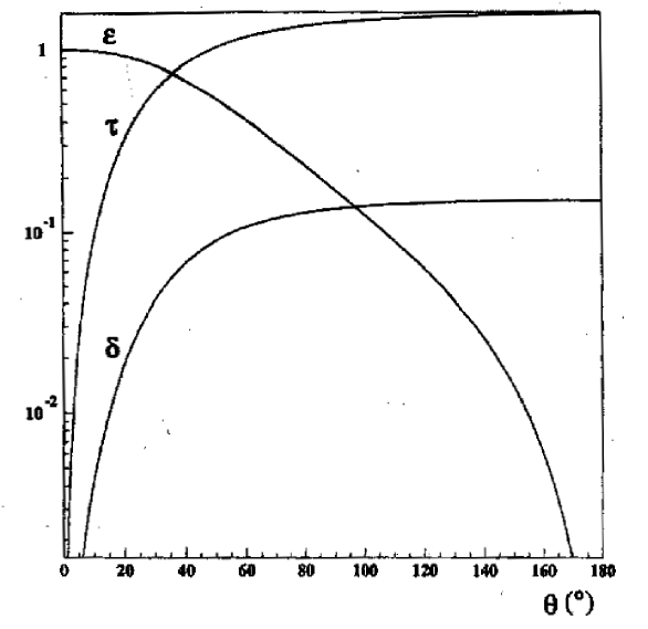
FIG. 17.: The kinematical coefficients $\tau$, $\varepsilon$ and $\delta$ versus the scattering angle $\theta$; the energy of the incoming electron is 3.355 GeV.

Equation (146) has already been exploited in experiments performed at Bates (SAMPLE) and CEBAF (HAPPEX) (see Refs. [43] and [44], respectively) for unraveling the strangeness content of the proton. Figure 17 may help in understanding the magnitudes of the quantities given above. There one infers that at backward scattering angles (SAMPLE) it is mainly the magnetic strangeness that is measured, however with some contamination arising from the axial contribution, whereas at forward angles (HAPPEX) it is a mixture of electric and magnetic strangeness that is observed, the axial contribution being totally negligible in that case.

Although the above discussions of strangeness content are focused on the responses of the nucleon rather than of the nucleus, in fact it is also relevant for the latter, since the nuclear responses measured in the quasielastic regime are indeed affected by the nucleon’s isoscalar form factors and these in turn are affected by strangeness. In fact this is an excellent example of how the theoretical predictions in nuclear many-body and particle physics are interrelated.

In particular, with regard to the responses of the nucleus, PV experiments offer the opportunity of

• disentangling the isoscalar and isovector contributions to $R_{\text{L}}^{\text{A}V}$, $R_{\text{T}}^{\text{A}V}$ and $R_{\text{T}^{\prime}}^{\text{V}A}$,

• exploring the Coulomb sum rule separately in the isoscalar and isovector channels (see Section IV),

• measuring the neutron distribution in nuclei (see Ref. [45]; not discussed here),

• investigating the nuclear axial response especially in the $\Delta$ region (also not discussed in the present work)

  and

• unambiguously revealing the role of the pion in nuclear excitations through the (possible) existence of a zero in the frequency behavior of the asymmetry.

To see how this occurs let us first split the PC and PV responses into their isospin components (we are neglecting the strangeness content at this point) according to

$$R_{\text{L},\text{T}}=\beta^{(0)}_{\text{V},EM}R^{I=0}_{\text{L},\text{T}}+\beta^{(1)}_{\text{V},EM}R^{I=1}_{\text{L},\text{T}}$$ (152)

$$R_{\text{L},\text{T}}^{\text{A}V}=\beta^{(0)}_{\text{V},WNC}R^{I=0}_{\text{L},\text{T}}+\beta^{(1)}_{\text{V},WNC}R^{I=1}_{\text{L},\text{T}}$$ (153)

for the vector channel. The PV axial channel is purely isovector at tree level. Next let us focus on the RFG model where the longitudinal isoscalar response is essentially proportional to $\left(G_{E}^{(0)}\right)^{2}=\left(G_{E_{p}}+G_{E_{n}}\right)^{2}$ and the isovector one to $\left(G_{E}^{(1)}\right)^{2}=\left(G_{E_{p}}-G_{E_{n}}\right)^{2}$. Since $G_{E_{n}}$ is small, especially at low $\tau$, it follows that

$$R^{I=0}_{\text{L}}\simeq R^{I=1}_{\text{L}}.$$ (154)

But then it is clear that the RFG PV longitudinal response is almost vanishing because of the opposite sign and approximately equal magnitude of the coefficients in Eqs. (139) and (140). This dramatic consequence of the Standard Model is displayed in Fig. 18, where the five responses entering in the definition of the asymmetry in Eq. (132) are shown for $|\mathchoice{{\hbox{\boldmath$\displaystyle q$}}}{{\hbox{\boldmath$\textstyle q$}}}{{\hbox{\boldmath$\scriptstyle q$}}}{{\hbox{\boldmath$\scriptscriptstyle q$}}}|$=300, 500 and 2000 MeV/c together with ${\cal A}$.

FIG. 18.: Relativistic Fermi gas response functions and asymmetry for ${}^{12}C$ at $q$=300 (a), 500 (b) and 2000 (c) MeV/c shown as functions of $\omega$. The location of $\omega=\frac{1}{2}|Q^{2}|/m_{N}$ is indicated by the arrow. Upper: the EM responses $R_{\text{L}}$ and $R_{\text{T}}$ are displayed. Middle: the parity-violating responses $R^{\text{A}V}_{\text{L}}$, $R^{\text{A}V}_{\text{T}}$ and $R^{\text{V}A}_{\text{T}^{\prime}}$ are shown. Lower: the asymmetry ${\cal A}$ is given for three values of the scattering angle $\theta$.

Beyond the fact that $R^{\text{A}V}_{\text{L}}$ is very small, one also observes in the figure that

• a similar cancellation does not occur in the transverse channel, where in fact the isoscalar and the isovector responses are quite different because now $(G_{M}^{(0)})^{2}\propto(\mu_{p}+\mu_{n})^{2}\simeq 0.77$ and $(G_{M}^{(1)})^{2}\propto(\mu_{p}-\mu_{n})^{2}\simeq 22.1$;

• $R^{\text{A}V}_{\text{T}}$ and $R^{\text{V}A}_{\text{T}^{\prime}}$ are negative, this being related to the sign of the axial coefficient of the leptonic WNC

  $$j_{\mu}(k^{\prime},s^{\prime};k,s)^{WNC}=\overline{u}(k^{\prime},s^{\prime})(a_{V}\gamma_{\mu}+a_{A}\gamma_{5}\gamma_{\mu})u(k,s),$$ (155)

  where $u(k,s)$ is the Dirac spinor of the electron. Indeed, according to the Standard Model,

  $$a_{V}=-(1-4\sin^{2}\theta_{W})\simeq-0.092\ \ \ \mbox{and}\ \ \ a_{A}=-1;$$ (156)

• as a consequence the asymmetry is negative as well, reflecting the left-handed nature of the weak interaction;

• the asymmetry, as previously mentioned, grows with $\tau$ and $\theta$.

How do interactions among the constituents of the RFG modify the above predictions?

B The role of the pion and other mesons

In answering the last question of the previous section we extend our model from a strict RFG framework to one where pions are also included [27], because then we can at least approximately preserve the two major requirements of Lorentz covariance and gauge invariance. Indeed the RFG cross section is built (apart from overall kinematical factors) from the contraction of the leptonic and hadronic Lorentz tensors and is therefore a relativistic invariant, although the partition into longitudinal and transverse responses depends, of course, upon the reference system. Moreover the single-nucleon four-current entering into the RFG nuclear tensor is conserved and hence the non-interacting RFG is gauge invariant.

When the nucleon-nucleon interaction carried by the pion is switched on it is not obvious that the two above mentioned properties are retained. Indeed, when the correlations and meson exchange currents (MEC) associated with the one pion exchange potential (OPEP) are introduced, as shown in Ref. [27] the Lorentz covariance and gauge invariance are violated (however, only slightly so) due to the following approximations that are usually made:

i) the pion propagator is assumed to be static,

ii) and a non-relativistic expansion of the two-body currents is performed [32].

In order to achieve a treatment of forces and currents that is as consistent as possible we first limit ourselves to the study of diagrams with only one pionic line, namely, we work in the first perturbative order in the N-N interaction. The correlation diagrams to be evaluated in this scheme are the so-called self-energy and exchange contributions, that when iterated to infinite order generate the previously discussed HF and RPA series, respectively. Note that the tadpole and ring diagrams vanish due to the spin and isospin structure of the OPEP. Concerning MEC, three contributions occur, the pion-in-flight term, the contact term and the one associated with the $\Delta$. A direct comparison with the exact relativistic calculation [46] shows that the non-relativistic expansion of Ref. [32] is indeed quite accurate up to momentum transfers of the order of 1 GeV/c.

The outcome of this is that sizable pionic contributions to the EM longitudinal (spin scalar, $\sigma=0$) and transverse (spin vector, $\sigma=1$) nuclear responses are found. In both cases the correlation effects produce a hardening of the responses, that is, a shift of the strength to higher $\omega$. The PV longitudinal and transverse correlated responses are simply obtained from the EM ones through the isospin rotations implied by the structure of the WNC discussed in the previous subsection; the axial-vector response will be treated separately in Section III C.

FIG. 19.: The longitudinal weak neutral current response $R_{\text{L}}^{\text{A}V}$ at $q$=500 MeV/c, showing the free RFG (dashed) and correlated (solid) results.

The main points emerging from this analysis are:

• In isospace the contribution of the self-energy diagram to the charge response is almost equally split between isoscalar ($I=0$) and isovector ($I=1$) components. The latter, on the other hand, is of course overwhelming in the transverse response, due to the dominance of the isovector magnetic moment. In contrast, in the case of the pionic force the $I=0$ part of the exchange diagram turns out to be three times as large as the $I=1$ one in the charge response and this imbalance, that becomes even stronger in higher orders of perturbation theory, is further strengthened by the difference between the isoscalar and isovector form factors. The isoscalar dominance of the pionic exchange correlations has dramatic consequences for the PV longitudinal response function, as may be seen in Fig. 19, where this response is displayed as a function of $\omega$ with and without pionic correlations.

  

  FIG. 20.: Feynman diagrams representing the free particle-hole polarization propagator for the EM (a) and PV (b) longitudinal response. The excitation of proton (p) and neutron (n) particle-hole pairs is shown separately. The labels strong and weak refer to the strength of the nucleon coupling to the photon $\gamma$ or to the vector boson $Z^{0}$.

  A physical interpretation of why $R_{\text{L}}^{\text{A}V}$ is small in the independent-particle model and why isospin-correlations are so important in determining its ultimate size follows from the expression for the observables in a language that explicitly refers to neutrons and protons rather than employing isospin labeling. Indeed, by inspecting Fig. 20, where the diagrams describing both the EM and PV longitudinal responses for a free system are displayed, one easily understands why in the non-interacting case the EM longitudinal response turns out to be substantial: both of its vertices can in fact be large, as they involve the coupling of a longitudinal photon to a proton. In contrast, one of the vertices entering in the non-interacting PV response is always small, since either the longitudinal coupling of a photon to a neutron or of a $Z^{0}$ to a proton is involved. This last fact is often phrased by saying that the $\gamma$ is blind to neutrons and the $Z^{0}$ is blind to protons (i.e., in the longitudinal channel). To quantify the meaning of “large” and “small” we note that typically the $\gamma-n$ coupling is about 1/10 that of the $\gamma-p$, and likewise the $Z^{0}-p$ coupling is about 1/10 that of the $Z^{0}-n$.

  The exchange correlations corresponding to the exchange of an isovector charged meson between the particle and hole convert a neutron (proton) into a proton (neutron), and thus give rise to a diagram where both couplings are large — hence the crucial role of such isovector correlations in determining $R_{\text{L}}^{\text{A}V}$.

  The above arguments clearly do not apply to the transverse response both because in this case the $I=0$ channel is much weaker than the $I=1$ channel, being essentially proportional to the squares of the very different isoscalar and isovector magnetic moments of the nucleon, and furthermore because protons and neutrons can both couple strongly to photons via their (comparable) magnetic moments. Being also essentially isovector, the axial-vector response likewise does not display the sensitivity expected for the longitudinal response.

• While the tensor component of the OPEP never contributes to the self-energy in a translationally invariant system, the exchange diagram gets a tensor contribution, but only in the transverse channel and mostly via the backward-going graphs. This implies a different role for the pionic force in the two EM responses, a finding that should be tested against experiment.

• When we extend our analysis from first to infinite order of perturbation theory, thus generating the HF and RPA responses, the results do not change substantially. Although the pionic interaction is strong, it nevertheless therefore appears that for quasielastic kinematics its effects are reasonably small at not too small $q$, thus rendering perturbation theory quite accurate already at the lowest order, at least for the classes of diagrams studied here.

• The contribution of the central part of the pionic interaction to the exchange diagram stems largely from the $\delta$-force and not from the finite-range one. Notably for pointlike nucleons the continuity equation is obeyed by the OPEP and by the related pionic MEC, but is not affected by its $\delta$ component. However in keeping with the usual approach taken in studies of pionic effects, we include a $\pi$NN vertex function $\Gamma_{\pi}$, whose scale is set by a mass parameter $\Lambda_{\pi}$, to smear out the $\delta$-piece of OPEP. As a consequence the continuity equation is modified by the presence of $\Gamma_{\pi}$ and to restore its validity additional MEC should be introduced. Significantly these counterterms affect only the pion-in-flight current, which is tiny, and therefore are quantitatively negligible.

• In contrast to the exchange diagram, the self-energy term gets a contribution only from momentum-dependent forces, and therefore an unmodified pionic $\delta$-interaction does not contribute in this channel. In fact, the contribution coming from the $\delta$-function in OPEP, when modified by the $\pi$NN vertex form factor, contains an effective momentum-dependence and so is nonzero.

• Most remarkably when the interactions carried by heavier mesons (namely $\rho$, $\sigma$ and $\omega$) are switched on, the previous conclusions on the PV responses (in particular the dramatic enhancement of $R_{\text{L}}^{\text{A}V}$) are not substantially changed, as illustrated in Ref. [14], thus showing the central role played by the pion in the nuclear dynamics for quasielastic kinematics. This is accomplished, however, through rather subtle aspects of the nuclear many-body problem, where the interference between the pion and the other mesons turns out to be crucial.

C The axial response and the asymmetry

Let us now turn to a discussion of the asymmetry in the pion-correlated Fermi gas model. For its evaluation the axial-vector response function $R_{\text{T}^{\prime}}^{\text{V}A}$ is needed. In a non-relativistic context the latter is related to the isovector component of the EM transverse response, $R^{\text{T}}_{{\text{A}V},I=1}$, through the simple formula [28]

$$R_{\text{T}^{\prime}}^{\text{V}A}(q,\omega)=a_{V}{G_{A}^{(1)}\over G_{M}^{(1)}}{1\over\kappa}R_{\text{T}}^{I=1}(q,\omega)\ ,$$ (157)

which can be extended into the relativistic regime via the prescription

$$R_{\text{T}^{\prime}}^{\text{V}A}(q,\omega)\cong a_{V}{G_{A}^{(1)}\over G_{M}^{(1)}}\sqrt{\tau+1\over\tau}R_{\text{T}}^{\text{I}=1}(q,\omega)\ ;$$ (158)

these agree to better than 2% in the momentum range 300 MeV/c $<q<1$ GeV/c for the RFG. Although not immediately apparent, Eq. (158) has been demonstrated to be preserved even in presence of pionic correlations. The effect of pionic correlations and MEC effects in this response is a “hardening” (a shift to higher $\omega$) of the peak of the response at intermediate values of $q$, which then fades away and even leads to a slight “softening” of the response at the highest momentum transfers considered.

We are now in the position to calculate the asymmetry ${\cal A}$, which is displayed in Fig. 21 as a function of $\omega$ for three values of $q$ and for forward ($\theta=10^{0}$) and backward ($\theta=170^{0}$) scattering angles.

FIG. 21.: The $\omega$-dependence of ${\cal A}$ for different kinematical conditions. The relativistic Fermi gas model results are labeled RFG, while the ones with pionic effects included are labeled $\pi$. The two families of curves have $g_{A}^{(1)}$=1.26 (solid), 1.26+10% (dashed) and 1.26-10% (dash-dotted).

Upon examining Fig. 21, we notice the significant effect occurring at moderate $q$ (say 300–500 MeV/c), small $\omega$ and forward angles. As previously discussed, it is related to the large negative value assumed by the correlated $R_{\text{L}}^{\text{A}V}$, which leads to a pionic asymmetry that is an order-of-magnitude larger than the free RFG one. However, as $\omega$ increases $R_{\text{L}}^{\text{A}V}$ rapidly decreases until it changes sign, while $R_{\text{T}}^{\text{A}V}$ stays negative; accordingly, they largely cancel in the numerator of the ratio expressing ${\cal A}$ and this becomes substantially lowered.

Interestingly, an energy is reached (about 60 MeV for $q=300$ MeV/c) where the correlated and free RFG values of ${\cal A}$ coincide. At still larger $\omega$ a further reduction of ${\cal A}$ is seen to occur until at about 90 MeV it nearly vanishes. This constitutes an example of a dynamical restoration of a symmetry (here the left-right parity symmetry) and reflects the complex nature of the PV longitudinal response. The near-vanishing of the asymmetry at $\omega\approx 90$ MeV in Fig. 21 stems from the cancellation between the positive contribution it gets from $R_{\text{L}}^{\text{A}V}$ and the negative one it gets from $R_{\text{T}}^{\text{A}V}$. This trend of course fades away at larger $\theta$, where the role of the longitudinal PV response gradually becomes irrelevant. Finally, we see that at larger momenta, where the impact of correlations is no longer so strongly felt, the nearly perfect restoration of the left-right symmetry does not show up anymore. It is, however, still true (even at 1 GeV/c) that an energy exists where the free and the correlated values of the asymmetry coincide.

From the lower panels of Fig. 21 it clearly appears that at backward angles ${\cal A}$ is almost equally sensitive to the nuclear dynamical effects and to the uncertainties in the nucleonic form factors. This raises the question of whether or not the asymmetry itself is a suitable observable for extracting information on either the nuclear correlations or the single-nucleon form factors. As a consequence we are led to consider three different integrated observables that have been introduced to emphasize one of the two aspects of the problem. They are:

• $$\Delta{\cal A}(q,\theta)\equiv{1\over{\Delta\omega}}\Bigl{[}\int_{\omega_{min}}^{\omega_{QEP}}\!\!d\omega{\cal A}(\theta;q,\omega)-\int_{\omega_{QEP}}^{\omega_{max}}\!\!d\omega{\cal A}(\theta;q,\omega)\Bigr{]}$$ (159)

• $${\overline{\cal A}}(q,\theta)\equiv{1\over{\Delta\omega}}\int_{\omega_{min}}^{\omega_{max}}\!\!d\omega\,{\cal A}(\theta;q,\omega)$$ (160)

  and

• $${\cal R}(q,\theta)\equiv{\int_{\omega_{min}}^{\omega_{max}}\!\!d\omega\ W^{PV}(q,\omega)\big{/}\widetilde{X}_{\text{T}}(\theta,\tau,\psi;\eta_{F})\over\int_{\omega_{min}}^{\omega_{max}}\!\!d\omega\ W^{EM}(q,\omega)\big{/}X_{\text{T}}(\theta,\tau,\psi;\eta_{F})}\,.$$ (161)

Here $\omega_{min}$ and $\omega_{max}$ are the RFG response boundaries for a fixed $q$

$$\omega_{min} = \sqrt{(k_{F}-q)^{2}+m_{N}^{2}}-\sqrt{k_{F}^{2}+m_{N}^{2}}$$ (162)

$$\omega_{max} = \sqrt{(k_{F}+q)^{2}+m_{N}^{2}}-\sqrt{k_{F}^{2}+m_{N}^{2}}\ ,$$ (163)

the energy interval $\Delta\omega$ is

$$\Delta\omega \equiv \omega_{max}-\omega_{min}$$ (164)

$$= \sqrt{(k_{F}+q)^{2}+m_{N}^{2}}-\sqrt{(k_{F}-q)^{2}+m_{N}^{2}}$$ (165)

$$\cong 2k_{F}q/\sqrt{q^{2}+m_{N}^{2}}$$ (166)

and the hadronic functions

$$W^{EM} = v_{\text{L}}R_{\text{L}}+v_{\text{T}}R_{\text{T}}$$ (167)

$$W^{PV} = v_{\text{L}}R_{\text{L}}^{\text{A}V}+v_{\text{T}}R_{\text{T}}^{\text{A}V}+v_{\text{T}^{\prime}}R_{\text{T}^{\prime}}^{\text{V}A}$$ (168)

are divided by

$$X_{\text{T}}(\theta,\tau,\psi;\eta_{F}) = v_{\text{T}}\left(2\tau G_{M}^{2}+\frac{G_{E}^{2}+\tau G_{M}^{2}}{1+\tau}\Delta\right)$$ (169)

$${\widetilde{X}}_{\text{T}}(\theta,\tau,\psi;\eta_{F}) = a_{A}v_{\text{T}}\left(2\tau G_{M}{\widetilde{G}_{M}}+\frac{G_{E}{\widetilde{G}}_{E}+\tau G_{M}{\widetilde{G}}_{M}}{1+\tau}\Delta\right)$$ (170)

in order to extract the single-nucleon content from the many-body one [47]. The quantity $\Delta$ is given later in Eq. (193): since $\Delta\sim\eta_{F}^{2}\ll 1$, the contributions containing $\Delta$ may often safely be neglected. Removing the single-nucleon content in this way has the following advantages:

FIG. 22.: The quantity $\Delta{\cal A}$ shown as a function of $\theta$ for $q$=300 (a), 500 (b) and 1000 MeV/c (c). The labeling of the curves is as in Fig. 21.

• The pionic correlations are particularly felt by $\Delta{\cal A}$, as is clearly apparent from Fig. 22. Indeed, there we first observe that at $q=300$ MeV/c the results obtained with the free RFG model almost vanish because of the nearly perfect cancellation between the contributions where $\omega<\omega_{QEP}$ and those where $\omega>\omega_{QEP}$; however, at larger $q$ this cancellation becomes less complete, owing partly to the role played by the nucleonic form factors and partly to the RFG model itself, whose responses (in contrast to the non-relativistic case) become less and less symmetric as $q$ increases. It is also clear that the correlations, in particular the exchange diagram, dramatically alter the prediction of the free RFG, yielding a huge $\Delta{\cal A}_{\pi}$ at small $\theta$. This result is simply interpreted by observing that of the nuclear responses that enter in the asymmetry the pion has its greatest effect on $R_{\text{L}}^{\text{A}V}$ and although in the RFG model the latter accounts only for at most about 10% of the total asymmetry (and this only in the forward direction), nevertheless the impact of the pionic correlations is violent enough to induce a large negative value of $R_{\text{L}}^{\text{A}V}$ at small $\omega$, which is in turn reflected in the large negative value of $\Delta{\cal A}_{\pi}$ at small $\theta$ displayed in Fig. 22. We deduce from this that the characteristic behavior of $\Delta{\cal A}$ with $\theta$ shown in the figure represents one of the most transparent signatures of pion-induced isoscalar correlations in nuclei (we recall that $R_{\text{T}^{\prime}}^{\text{V}A}$ is purely isovector and that in $R_{\text{T}}^{\text{A}V}$ the isoscalar contribution is strongly suppressed — see Ref. [27]).

  The observable $\Delta{\cal A}$ has been specifically devised to enhance the signal for nuclear correlations and to minimize the sensitivity to the single-nucleon form factors. This can be inferred by observing the three (almost overlapping) lines for each family of curves in Fig. 22, corresponding to a variation of the strength of the effective axial-vector coupling, $g^{(1)}_{A}$, of $\pm 10$% around the canonical value $g^{(1)}_{A}=1.26$. The impact on $\Delta{\cal A}$ of pionic correlations is seen to be more than an order-of-magnitude larger than that arising from variations in the axial-vector form factor. Similar results are found for the magnetic and electric strangeness form factors (see Ref. [28]).

• The energy-averaged asymmetry ${\overline{\cal A}}$, on the other hand, has been devised to minimize the sensitivity to the pionic correlations, as these tend to cancel out in the symmetrical integral in Eq. (160). The MEC contribution, on the other hand, does not average out in ${\overline{\cal A}}$, although in the $ph$ sector of the nuclear excitations it turns out to have a rather insignificant effect. Typical results are shown in Fig. 23 for $q=$ 500 MeV/c.

  

  FIG. 23.: The energy-averaged asymmetry ${\overline{\cal A}}$ displayed as a function of $\theta$ for $q$=500 MeV/c, with the same labeling of the curves as in Fig. 21. Panel (a) shows the entire angular range, while (b) only shows the backward-angle region in greater detail.

  In particular, as seen in the expanded view in the figure, at very backward scattering angles where one might hope to determine the effective axial-vector coupling $g_{A}^{(1)}$ (again variations of $\pm 10$% around 1.26 are shown in the figure) the free RFG and pionic correlated results for the energy-averaged asymmetry come together (for $q$=500 MeV/c at $\theta\approx 147^{o}$, which however varies with $q$). Since this special condition is presumably model-dependent, it is unlikely that one can count on using such particular kinematics to effect a determination of $g_{A}^{(1)}$ through the variations shown in the figure.

  In contrast to the backward-angle situation, at forward scattering angles where the pionic correlations induce drastic modifications in $R_{\text{L}}^{\text{A}V}$, as we have seen, here the two families of curves differ although certainly not as much as in the case of $\Delta{\cal A}$. In other words, the observable ${\overline{\cal A}}$ has some of the properties that we are looking for when we construct quantities that suppress the effects of correlations while bringing out the dependences on the single-nucleon form factors; however, this particular observable appears not to be entirely optimal. Since the PV longitudinal response is so strongly affected by the presence of pionic correlations, it is necessary to adopt an alternative approach to minimize these effects, leading to the introduction of the observable in Eq. (161).

  

  FIG. 24.: The quantity ${\cal R}$ versus $\theta$ for $q$=300 (a), 500 (b) and 1000 MeV/c (c). The curves are labeled as in Fig. 21.

• The procedure proposed in Refs. [28, 47] for the definition of the quantity ${\cal R}$ has the goal of scaling the results (see the next section) by dividing out most of the single-nucleon content through the use of the dividing factors $X_{\text{T}}$ and ${\widetilde{X}}_{\text{T}}$. In Fig. 24 we show ${\cal R}$ as a function of $\theta$ for three values of $q$. Again two families of curves are displayed, one for the free RFG and one for the model with pionic effects included (labeled $\pi$), and each family has three curves ($g_{A}^{(1)}=1.26$, $1.26+10$% and $1.26-10$%). In panel b we see a significant range of angles over which the pionic effects provide negligible modifications with respect to the RFG results and where the (merged) curves with the three values of the isovector/axial-vector strength can clearly be discerned. This behavior is similar at $q=1$ GeV/c, although not quite as nicely separated. Even so, the difference between the RFG and pionic families at backward scattering angles amounts to an effective change in $g_{A}^{(1)}$ of only about 4%.

  It thus appears that the observable ${\cal R}$ is sufficiently uncontaminated by correlation effects for favorable kinematics and better suited than ${\overline{\cal A}}$ to disentangling the nucleonic form factors from the nuclear dynamics. It has been specifically designed to integrate out the anomalous $\omega$-dependence, leaving quantities that for the most part only retain sensitivities to variations in the single-nucleon form factors.

IV Scaling and sum rules

In this section we briefly address several issues that arise in discussing scaling and sum rules, showing how these two properties are interrelated and how they constrain the nuclear models. At sufficiently large three-momentum transfer $q$ the so-called $y$-scaling region occurs when the energy transfer $\omega$ is lower than its value at the quasielastic peak and when non-quasielastic processes such as meson production do not affect the nuclear responses. The $y$-scaling approach attempts to find some function of $q$ and $\omega$, here denoted $G$, such that when divided into the inclusive electron scattering cross section, the result is a reduced response $F(q,y)$ that scales as a function of $y$. Here $y$ is an appropriately chosen scaling variable (see below), is a function of $(q,\omega)$ and replaces $\omega$ (i.e., one uses the variables $q$ and $y$, rather than $q$ and $\omega$). “Scaling” means that for sufficiently large momentum transfers the function $F$ becomes universal, namely a function only of $y$, but not of $q$:

$$F(q,y)\stackrel{{\scriptstyle q\to\infty}}{{\longrightarrow}}F(y)\equiv F(\infty,y).$$ (171)

The choice of the dividing function and scaling variable must be such as to remove the single-nucleon content from the nuclear responses in as model-independent a manner as possible while still retaining essential relativistic effects whenever feasible.

A parallel strategy concerns the Coulomb Sum Rule (CSR) [39, 48]: a dividing function $H_{\text{L}}$ can be devised such that the corresponding reduced longitudinal response $r_{\text{L}}=R_{\text{L}}/H_{\text{L}}$ fulfills the CSR.

In past work medium- and high-energy data have been tested with both the usual $y$-scaling approach (for a review, see Ref. [49]), while more recently the RFG-motivated approach has been applied and seen to scale successfully [3, 50, 51]. Actually these data appear to support not only scaling, but also superscaling, namely the existence of a function related to $F$ that is the same for all nuclei [47, 50, 51]. Additionally, it now appears that the experimental CSR is reasonably well saturated at high momentum transfers [1]. As a consequence, any reliable nuclear model should simultaneously fulfill the two major requirements of

1) scaling

2) fulfilling the Coulomb Sum Rule.

We now show that the RFG model simultaneously satisfies the above properties. In the context of the PWIA for $(e,e^{\prime}N)$ reactions the $y$-scaling variable is defined to be equal and opposite to the smallest value of the missing momentum, $p_{min}$, attained in the $y$-scaling region: It turns out to read

$$y = -p_{min}=\frac{1}{2W^{2}}\left\{\left(M^{0}_{A}+\omega\right)\sqrt{W^{2}-\left(M^{0}_{A-1}+m_{N}\right)^{2}}\sqrt{W^{2}-\left(M^{0}_{A-1}-m_{N}\right)^{2}}\right.$$ (173)

$$-\left.q\left[W^{2}+\left(M^{0}_{A-1}\right)^{2}-m_{N}^{2}\right]\right\},$$

where

$$W=\sqrt{\left(M^{0}_{A}+\omega\right)^{2}-q^{2}},$$ (174)

$M^{0}_{A}$ and $M^{0}_{A-1}$ being the masses of the initial and daughter nuclei (in their ground states), respectively. The energy transfer can, of course, be expressed in terms of $q$ and $y$. In particular, it must lie in the range [39] $\omega_{t}\leq\omega\leq q$, where

$$\omega_{t}=E_{S}+\sqrt{(M^{0}_{A-1}+m_{N})^{2}+q^{2}}-(M^{0}_{A-1}+m_{N})$$ (175)

is the threshold energy, with $E_{S}=m_{N}+M^{0}_{A-1}-M^{0}_{A}$ being the nuclear separation energy. The scaling variable in Eq. (173) vanishes when

$$\omega=\omega_{0}=E_{S}+\sqrt{m_{N}^{2}+q^{2}}-m_{N},$$ (176)

which is roughly the position of the quasielastic peak, and hence the scaling region is characterized by having $y$ negative.

In order to study the scaling behavior of the inclusive $(e,e^{\prime})$ process one should be able to remove the effective $eN$ cross section from under the integrals involved in going from coincidence to inclusive scattering. These integrals extend over the missing momentum $(p_{m})$ and over an energy that characterizes the degree of excitation of the daughter nucleus, ${\cal E}$:

$${\cal E}=E_{A-1}-E_{A-1}^{0}\geq 0,$$ (177)

where $E_{A-1}$ is the energy of the unobserved daughter system (in general in an excited state) and $E_{A-1}^{0}$ is that energy when this system is in its ground state, i.e., has mass $M_{A-1}^{0}$. Naturally ${\cal E}$ can be re-expressed in terms of the missing energy $E_{m}$; one has roughly that $E_{m}\cong{\cal E}+E_{S}$. If one assumes that the proton and neutron distributions inside the nucleus are equal, which is a reasonable approximation for $N=Z$ nuclei, and that the most important contributions to the nuclear spectral function arise from the lowest values of $(p,{\cal E})$ that can be reached for given values of $q$ and $y$ (in the scaling region these are ${\cal E}=0$ and $p=-y$), then the function one hopes will scale as a function of $y$ when $q\rightarrow\infty$ is

$$F(q,y)\equiv\frac{d^{2}\sigma/d\Omega_{e}d\omega}{{\tilde{\sigma}}_{eN}(q,y;p=-y,{\cal E}=0)}.$$ (178)

In the PWIA this is indeed found to be the case, since in the limit $q\to\infty$ Eq. (178) becomes a function only of $y$, namely it scales [49].

Turning now to the RFG model, its spectral function [39] is

$$\tilde{S}^{\text{RFG}}(p,{\cal E})=\frac{3A}{8\pi k^{3}_{F}}\theta(k_{F}-p)\delta\left[{\cal E}(p)-{\cal E}^{\text{RFG}}(p)\right],$$ (179)

where the excitation energy is

$${\cal E}^{\text{RFG}}(p)=\left(\sqrt{k^{2}_{F}+m_{N}^{2}}-\sqrt{p^{2}+m_{N}^{2}}\right)\ .$$ (180)

Defining the RFG scaling variable through the intercept of the support of the RFG spectral function given in Eq. (179) and the kinematical boundaries in the missing energy-missing momentum plane one obtains the $y$-scaling variable of RFG

$$y_{\text{RFG}}=m_{N}\zeta=m_{N}\left(\lambda\sqrt{1+\frac{1}{\tau}}-\kappa\right),$$ (181)

where the dimensionless variables $\lambda=\omega/2m_{N}$, $\kappa=q/2m_{N}$ and $\tau=\kappa^{2}-\lambda^{2}$ have been introduced.

A different scaling variable was originally proposed for the RFG in Ref. [47], namely

$$\psi=\frac{1}{\sqrt{\xi_{F}}}\frac{\lambda-\tau}{\sqrt{(1+\lambda)\tau+\kappa\sqrt{\tau(1+\tau)}}},$$ (182)

where $\xi_{F}=\epsilon_{F}-1=\sqrt{1+\eta_{F}^{2}}-1$ and $\eta_{F}=k_{F}/m_{N}$ are the dimensionless Fermi kinetic energy and momentum, respectively. With some algebra it can be shown that the relation between the two scaling variables is

$$\xi_{F}\psi^{2}=\sqrt{1+(y_{\text{R}FG}/m_{N})^{2}}-1.$$ (183)

The physical significance of $\psi$ is then immediately apparent: among the nucleons responding to an external probe one has the smallest kinetic energy and this is given by $\psi^{2}$ (in units of the dimensionless Fermi kinetic energy $\xi_{F}$). Instead of working from the unseparated inclusive cross section towards a reduced response that, if successful, would scale as $q\to\infty$, one can work directly with the separated longitudinal and transverse responses, $R_{\text{L}}$ and $R_{\text{T}}$, since

• we are most interested in model-to-model comparisons and the same procedures may be followed in each case (i.e., focusing on L or T responses directly),

• a few cases exist where L/T separations have been performed experimentally,

• we wish to draw comparisons with studies of the CSR where only the $L$ response is relevant.

In this spirit we seek reduced responses denoted $F_{\text{L},T}(\kappa,\psi)$ that scale. These are to be obtained from the inclusive response functions $R_{\text{L},T}(\kappa,\lambda)$ by dividing through by specific functions, denoted $G_{\text{L},T}(\kappa,\lambda)$:

$$F_{\text{L},T}(\kappa,\psi)\equiv R_{\text{L},T}(\kappa,\lambda)/G_{\text{L},T}(\kappa,\lambda).$$ (184)

If the dividing functions are chosen appropriately, then as above the reduced responses defined in Eq. (184) will scale, namely, become functions only of a single scaling variable such as $\psi$ defined above when $\kappa\rightarrow\infty$,

$$F_{\text{L},T}(\kappa,\psi)\stackrel{{\scriptstyle\kappa\to\infty}}{{\longrightarrow}}F_{\text{L},T}(\psi)\equiv F_{\text{L},T}(\infty,\psi).$$ (185)

Such dividing functions, derived in Ref. [52, 39], are

$$G_{\text{L}}(\kappa,\lambda) = \frac{ZU_{\text{L}p}+NU_{\text{L}n}}{2\kappa[1+\xi_{F}(1+\psi^{2})/2]}$$ (186)

$$= \frac{1}{2\kappa}(ZU_{\text{L}p}+NU_{\text{L}n})+{\cal O}(\xi_{F})$$ (187)

and

$$G_{\text{T}}(\kappa,\lambda) = \frac{ZU_{\text{T}p}+NU_{\text{T}n}}{2\kappa[1+\xi_{F}(1+\psi^{2})/2]}$$ (188)

$$= \frac{1}{2\kappa}(ZU_{\text{T}p}+NU_{\text{T}n})+{\cal O}(\xi_{F}),$$ (189)

where (see Ref. [53])

$$U_{\text{L}p,n}=\frac{\kappa^{2}}{\tau}\left[G_{\text{E}p,n}^{2}(\tau)+W_{2{\text{p},n}}(\tau)\Delta\right]$$ (190)

$$U_{\text{T}p,n}=2\tau G_{\text{M}p,n}^{2}(\tau)+W_{2\text{p,n}}(\tau)\Delta\ ,$$ (191)

with

$$W_{2{\text{p},n}}(\tau)=\frac{1}{1+\tau}\left[G_{\text{E}p,n}^{2}(\tau)+\tau G^{2}_{\text{M}p,n}(\tau)\right]$$ (192)

and

$$\Delta=\frac{\tau}{\kappa^{2}}\left[\frac{1}{3}\left(\epsilon^{2}_{F}+\epsilon_{F}\sqrt{1+\zeta^{2}}+1+\zeta^{2}\right)+\lambda\left(\epsilon_{F}+\sqrt{1+\zeta^{2}}\right)+\lambda^{2}\right]-(1+\tau).$$ (193)

Dividing the longitudinal and transverse RFG response functions by $G_{\text{L}}$ and $G_{\text{T}}$ yields the reduced responses

$$F_{\text{L}}^{\text{RFG}}(\psi)=F_{\text{T}}^{\text{RFG}}(\psi)=\frac{3\xi_{F}}{2m_{N}\eta^{3}_{F}}(1-\psi^{2})\theta(1-\psi^{2})\left[1+\frac{1}{2}\xi_{F}(1+\psi^{2})\right],$$ (194)

that, by construction, scale with $\psi$, $\zeta$ or $y_{\text{R}FG}$.

In parallel with the scaling behavior of the RFG one can study the CSR and the various energy-weighted moments of another reduced response denoted $r_{\text{L}}(\kappa,\lambda)$, introduced in Refs. [47, 39]. Here the longitudinal response $R_{\text{L}}(\kappa,\lambda)$ is divided by a function $H_{\text{L}}(\kappa,\lambda)$ to yield

$$r_{\text{L}}(\kappa,\psi)\equiv R_{\text{L}}(\kappa,\lambda)/H_{\text{L}}(\kappa,\lambda)$$ (195)

and the n^th moment of the longitudinal response of the nucleus is given by

$$\Xi^{(n)}=\int\limits_{0}^{\kappa}d\lambda\,\lambda^{n}\,r_{\text{L}}(\kappa,\lambda).$$ (196)

In particular, the $n=0$ moment, $\Xi^{(0)}$, is the CSR. In the case of the RFG the dividing function is

$$H_{\text{L}}(\kappa,\lambda)=\frac{\kappa\eta_{F}^{3}}{2\xi_{F}}\left(ZU_{\text{L}p}+NU_{\text{L}n}\right)/\left(\partial\psi/\partial\lambda\right)\ .$$ (197)

Thus, upon dividing the charge response of the RFG by Eq. (197) one obtains the following reduced longitudinal response

$$r^{\text{RFG}}_{\text{L}}(\kappa,\lambda)=\frac{3}{8m_{N}}(1-\psi^{2})\theta(1-\psi^{2})\frac{{\partial\psi}}{\partial\lambda},$$ (198)

which, by construction, fulfills the CSR in the non-Pauli-blocked domain, as can easily be verified.

The two dividing functions $G_{\text{L}}$ (related to the scaling) and $H_{\text{L}}$ (related to the CSR) are linked according to [39]

$$G_{\text{L}}(\kappa,\lambda) = \left(\frac{\eta^{3}_{F}}{4\xi_{F}}\right)\frac{\partial\psi}{\partial\lambda}\frac{1}{1+\xi_{F}(1+\psi^{2})/2}H_{\text{L}}(\kappa,\lambda)$$ (199)

$$= \frac{1}{2}\left(\frac{\kappa}{\tau}\right)\left(\frac{1+2\lambda}{1+\lambda}\right)H_{\text{L}}(\kappa,\lambda)+{\cal O}(\xi_{F}).$$ (200)

When experimental data are reduced using the above dividing functions, they are seen to yield a CSR at high-$q$ and to scale when plotted versus any of the scaling variables previously introduced.

Finally we explore the scaling and CSR properties of nuclear models other than the RFG, specifically:

• the hybrid model (HM), introduced in Ref. [39];

• the quantum hadrodynamical (QHD) model [54].

The hybrid model is designed to account for the binding of the nucleons inside the nucleus, thus curing a flaw of the RFG related to its negative separation energy. The HM has continuum states that are plane waves, as in the RFG model, but has bound states described by shell-model wave functions obtained by solving the Schrödinger equation with some choice of potential well (in [39] harmonic oscillator bound-state wave functions were used to simplify the analysis in the limit where $A\to\infty$). In the HM the scaling variable cannot be obtained analytically, since the model can only be treated numerically. However, scaling variables exist that incorporate the shift result from using Eq. (181) for $\zeta^{\prime}$ (and a corresponding dimensionful variable $y^{\prime}$) or Eq. (182) for $\psi^{\prime}$ by making the replacements $\lambda\to\lambda^{\prime}$ and $\tau\to\tau^{\prime}=\kappa^{2}-{\lambda^{\prime}}^{2}$, where

$$\lambda^{\prime}=\lambda-\lambda_{\text{shift}},$$ (201)

with

$$\lambda_{\text{shift}}=\frac{1}{2m_{N}}(T_{F}+E_{S})$$ (202)

and $T_{F}=m_{N}\xi_{F}$ the Fermi kinetic energy. The HM turns out to have the width of its reduced response identical to a RFG computed with a Fermi momentum that is somewhat larger than the usual one (237 MeV/c for the HM, versus the 230 MeV/c value for $k_{F}$ used for the RFG to correspond to nuclei near ⁴⁰Ca or ⁵⁶Fe).

Scaling may then be examined for the HM by computing

$$F^{\text{HM}}_{\text{L}}(\kappa,\psi)\equiv R^{\text{HM}}_{\text{L}}(\kappa,\lambda)/G_{L}(\kappa,\lambda)$$ (203)

and the various energy-weighted moments of the longitudinal response, including the zeroth moment or CSR, may be computed using

$$r^{\text{HM}}_{\text{L}}(\kappa,\psi)\equiv R^{\text{HM}}_{\text{L}}(\kappa,\lambda)/H_{\text{L}}(\kappa,\lambda).$$ (204)

Note that the same dividing factors $G_{\text{L}}$ and $H_{\text{L}}$ that were developed from our discussions of the RFG are used.

FIG. 25.: The reduced response $F^{\text{HM}}_{\text{L}}$ (the hybrid model scaling function) is shown as a function of $\psi$ in panel (a) and $\psi^{\prime}$ in panel (b) for 4 values of $q$ (fine dotted — 0.5, dot-dashed — 1.0, heavy solid — 1.5 and solid — 2.0 GeV/c). The RFG result, which scales exactly as a function of $\psi$, is also shown for reference as a dashed curve in panel (a).

In Fig. 25 the scaling function $F^{\text{HM}}_{\text{L}}$ for ⁴⁰Ca is displayed versus $\psi$ and $\psi^{\prime}$ for four different values of $q$ (the RFG result is also shown for reference): the HM scales either with $\psi$ or with $\psi^{\prime}$ as $q$ becomes large. Indeed, only the $q=$ 500 MeV/c plot versus $\psi$ shows any appreciable violation of scaling, whereas the scaling versus $\psi^{\prime}$ is excellent.

In the QHD model [54] protons and neutrons in the nucleus are described by Dirac spinors and move in strong Lorentz scalar and vector mean fields. These in turn arise self-consistently from the exchange of $\sigma$ and $\omega$ mesons between the same nucleons on which they act. The scalar field dresses the bare mass of the nucleon, considerably lowering its value; the vector field uniformly shifts the fermion spectrum. As a consequence the QHD charge response of nuclear matter in Hartree approximation is unaffected by the vector field, while it turns out to be quite sensitive to the effective mass $m^{\ast}_{N}$ induced by the scalar field. This is, of course, true in the simple approximation of constant relativistic mean fields. An improved description allows for an energy-dependence of the latter, which helps to account for the data of proton-nucleus elastic scattering.

As for the HM model, scaling can be examined in the QHD model by computing

$$F^{\text{QHD}}_{\text{L}}(\kappa,\psi)\equiv R^{\text{QHD}}_{\text{L}}(\kappa,\lambda)/G_{\text{L}}(\kappa,\lambda)$$ (205)

and likewise the various energy-weighted moments of the longitudinal response computed using

$$r^{\text{QHD}}_{\text{L}}(\kappa,\psi)\equiv R^{\text{QHD}}_{\text{L}}(\kappa,\lambda)/H_{\text{L}}(\kappa,\lambda).$$ (206)

Since the dividing factors are (at least to a very good level of approximation) universal, accordingly we use the same dividing factors $G_{\text{L}}$ and $H_{\text{L}}$ that were developed from our discussions of the RFG.

FIG. 26.: The reduced response $F^{\text{QHD}}_{\text{L}}$ with $m_{N}^{\ast}=$ 0.68 $m_{N}$ is shown as a function of $\psi$ in panel (a) and $\psi^{\ast}$ in panel (b) for 4 values of $q$ (fine dotted — 0.5, dot-dashed — 1.0, heavy solid — 1.5 and solid — 2.0 GeV/c). The RFG result, which scales exactly as a function of $\psi$, is also shown for reference as a dashed curve in panel (a).

In Fig. 26 we display the reduced responses in Eqs. (205) and (206) as functions both of $\psi$ and also $\psi^{\ast}$, namely, the RFG scaling variable given in Eq. (182) with $m_{N}$ replaced by $m_{N}^{\ast}$ (two different values of the effective mass, $m_{N}^{\ast}=0.68\,m_{N}$ and 0.8 $m_{N}$ are used). It is clearly seen that $F^{\text{QHD}}_{\text{L}}$ does not scale versus $\psi$ when the effective mass is constant and differs from $m_{N}$. As $q$ continues to grow beyond the range of values shown in the figures, the results continue to shift to higher $\omega$ and never coalesce into a universal curve. When plotted versus $\psi^{\ast}$ the behavior, while better, still does not scale. This is in contrast with the RFG and HM results displayed above and, importantly, is not what is seen experimentally where the world data do appear to scale in $\psi$ [51]. The fact that experimentally the scaling is observed to occur successfully for $q$ greater than about 1 GeV/c suggests that $m_{N}^{\ast}/m_{N}$ should not deviate appreciably from unity for such kinematics.

Finally, the CSR ($\Xi^{(0)}$), the energy-weighted sum rule ($\Xi^{(1)}/\Xi^{(0)}$) and the variance $\sigma=\sqrt{\Xi^{(2)}-(\Xi^{(1)})^{2}}$ of ⁴⁰Ca corresponding to the HM, QHD (with $m_{N}^{\ast}=0.68$ $m_{N}$ and 0.8 $m_{N}$) and RFG models are displayed in Fig. 27. The RFG model and the HM both saturate the CSR at high-$q$. In contrast, the QHD model does so only if the effective value of $m_{N}^{\ast}/m_{N}$ evolves with increasing $q$ towards unity, as suggested by the latest version of the model.

FIG. 27.: The Coulomb sum rule (a), energy-weighted sum rule (b) and variance (c) are shown as functions of $q$ for three models: dashed — the RFG, solid — the HM and the QHD model with $m_{N}^{\ast}$=0.8 $m_{N}$ (dot-dashed) and 0.68 $m_{N}$ (dotted).

V Outlook and perspectives

In this paper we have discussed the parity-conserving and violating- inclusive nuclear responses, addressing the following issues

• Where do they occur?

• How can we describe them?

• What is their input?

With respect to the first item we have limited our focus to the quasielastic peak (QEP), since at larger excitation energies where for example the $\Delta$ plays a role we do not expect a description of the nucleus only in terms of nucleonic and mesonic degrees of freedom to be adequate. At some point QCD degrees of freedom should become the more appropriate ones to describe inclusive scattering. On the other hand at energies significantly lower than those characterizing the QEP where discrete excitations, giant resonances, etc. are seen the theoretical many-body framework is different from the one used here.

Concerning the second item let us again stress that any theoretical framework should first fulfill (as much as possible) Lorentz covariance and gauge invariance. For this the RFG appears to be a good starting point: It is a covariant model, since its ingredients are the fully relativistic nucleon propagators and EM (or WNC) vertices, and it respects gauge invariance, since the vector currents of the nucleon are conserved. When mesons are added to the picture then Lorentz covariance and gauge invariance are fulfilled to the extent that one allows for a dynamical propagation of the mesons and treats the forces and the currents consistently. This turns out to be possible for the case of the pion.

Of course the RFG misses surface and finite-size effects; however, first of all, these are of minor relevance for the scattering of electrons in the QEP and $\Delta$ peak domains, and secondly, they can be satisfactorily accounted for within the semiclassical approach, which exploits the advantages offered by the translational invariance of the RFG and accommodates these advantages to fit the physics of finite systems [56].

In the framework of the RFG we have treated nucleon-nucleon correlations in a perturbative scheme. Alternatives are represented by

• variational approaches

• loop expansions in the path integral framework, which however represent an alternative regrouping of perturbation theory.

Concerning perturbation theory we have seen that basic ingredients are the diagrams associated with the HF mean field and those related to the antisymmetrized RPA. The emphasis on the antisymmetrization arises from the recognition that very important carriers of the nuclear force, notably $\pi$ and $\rho$ mesons, only act through the exchange diagrams.

The short-range correlations (SRC) induced by the violent repulsion present in the N-N force at small distances are then inserted via the ladder diagrams. It is, however, doubtful whether ladders can be covariantly computed, especially at high densities (or Fermi momenta $k_{F}$) where they become increasingly important and the role of relativity cannot be ignored. In addition, it may be that searching for a totally deterministic account of the N-N correlations is not the optimal way to proceed — should, for example, quantum chaos be at work in atomic nuclei, then costly efforts to compute SRC would not represent the most efficient way of interpreting the nuclear response functions.

A further serious challenge facing the perturbative approach relates to the estimate of the size of diagrams that are not considered. In this connection it appears that only the loop expansion offers a consistent criterion (the number of loops) to organize the perturbative series in classes of homogeneous diagrams allowing at the same time an estimate of the rate of convergence of the resulting new expansion. However, although this is theoretically established, its practical implementation is far from trivial.

Finally a few words on the input to be fed into the perturbative scheme are appropriate. In general the Bonn potential appears as a well-founded representation of the N-N force. Indeed it provides an excellent representation of the energy behavior of the N-N phase shifts in free space and of the deuteron’s properties. In addition, it can be derived from a Lagrangian defined in terms of nucleonic and mesonic fields, and therefore cast in the framework of an effective field theory that, from the theoretical viewpoint, represents a highly desirable feature. In particular, it allows for a test of the gauge invariance of the theory, i.e. the consistency between the forces and currents. In this connection it is worthwhile to emphasize that the most direct way to assess the validity of the mesons-plus-nucleons model of the nucleus ultimately rests on a deeper understanding of the role of meson exchange currents (MEC) in the nuclear responses. Much has been done in this field, although much remains to be done.

It seems to us that at present the analysis of the nuclear responses is best performed on the basis of a hadronic approach such as the one we have pursued using the Bonn potential. It is important to remember, however, that such potentials are being used for nucleons within the nucleus and that these are differently off-shell from the conditions found in studying N-N scattering or the ground state of the deuteron.

In summary, in Section II of the present article we have analyzed the quasielastic response functions for inclusive electron scattering in the standard framework of HF plus RPA. In addition, the impact of short-range correlations on the effective particle-hole force has been explored within the context of the G-matrix approach. The analysis has then been extended in Section III to include the observables that occur in studying parity-violating electron scattering, with emphasis placed on the “new” nuclear axial response. In Section IV the attention has been directed towards several general, important properties of the response functions, in particular their Coulomb sum rule and scaling/superscaling behavior. Finally, a short account of what lies ahead has been provided in Section V.

A Electromagnetic form factors of the nucleon

Here we give the formulae for the EM form factors introduced in the definition of the response functions in Eq. (19).

1 Non-relativistic Fermi gas

In a non-relativistic calculation one defines, in terms of Sach’s form factors,

$${f_{L}^{(I)}}^{2} = {G_{E}^{(I)}}^{2}$$ (A2)

$${f_{T}^{(I)}}^{2} = 2\tau{G_{M}^{(I)}}^{2},\qquad I=0,1,$$ (A3)

where $\tau=|Q^{2}|/4m_{N}^{2}=(q^{2}-\omega^{2})/4m_{N}^{2}$, $G^{(I)}_{X}=G_{X_{p}}+(-1)^{I}G_{X_{n}}$ ($X=E,M$). A typical parameterization (although many others are possible) is the dipolar-plus-Galster one, namely

$$\begin{array}[]{lcl}G_{E_{p}}(\tau)&=&G_{D}^{V}(\tau)\\ G_{M_{p}}(\tau)&=&\mu_{p}G_{D}^{V}(\tau)\\ G_{M_{n}}(\tau)&=&\mu_{n}G_{D}^{V}(\tau)\\ G_{E_{n}}(\tau)&=&-\mu_{n}\tau G_{D}^{V}(\tau)\xi_{n}(\tau).\end{array}$$ (A4)

Here $G_{D}^{V}(\tau)=(1+\lambda_{D}^{V}\tau)^{-2}$ is the vector dipole form factor, with $\lambda_{D}^{V}\cong 4.97$, whereas $\mu_{p}\cong 2.793$ and $\mu_{n}\cong-1.913$ are the proton and neutron magnetic moments, respectively. For $G_{E_{n}}$ we have adopted the Galster parameterization [55] with $\xi_{n}(\tau)=(1+\lambda_{n}\tau)^{-1}$ and $\lambda_{n}\cong 5.6$.

2 Relativistic Fermi gas

In Ref. [32] it was shown that in an RFG calculation a very good approximation to the exact treatment of the EM vertices can be obtained with the following definitions:

$${f_{\text{L}}^{(I)}}^{2} = \left[\frac{1}{1+\tau}{G_{E}^{(I)}}^{2}+\tau{G_{M}^{(I)}}^{2}\frac{k_{F}^{2}}{2m_{N}^{2}}(1-\psi_{r})^{2}\right],$$ (A6)

$${f_{\text{T}}^{(I)}}^{2} = \frac{2\tau}{(1+\omega/2m_{N})^{2}}{G_{M}^{(I)}}^{2},$$ (A7)

where $\psi_{r}$ is the relativistic scaling variable in Eq. (24), $k_{F}$ is the Fermi momentum and the other quantities have been defined in Eqs. (A4).

B First-order self-energy

Here we give the analytic expressions for the first-order self-energy based on the potential in Eqs. (2)–(* ‣ II A). $\Sigma^{(1)}(k)$ is the sum of direct (“Hartree”) and exchange (“Fock”) terms, namely

$$\Sigma^{(1)}(k)\equiv\Sigma^{\text{H}}(k)+\Sigma^{\text{F}}(k),$$ (B1)

where

$$\Sigma^{\text{H}}(k)=\rho V_{0}(0)$$ (B2)

and

$$\Sigma^{\text{F}}(k)=-\frac{3}{8}\rho\sum_{\alpha}C^{(\alpha)}_{\text{F}}{\cal S}^{\text{F}}_{\alpha}(k),$$ (B3)

$\rho=2k_{F}^{3}/3\pi^{2}$ being the nuclear density. In the last equation we have introduced the spin-isospin coefficients (note that the tensor channels do not contribute)

$$C^{(0)}_{\text{F}} = 1,\quad C^{(\tau)}_{\text{F}}=3,\quad C^{(\sigma)}_{\text{F}}=3,\quad C^{(\sigma\tau)}_{\text{F}}=9,$$ (B4)

$$C^{(t)}_{\text{F}} = C^{(t\tau)}_{\text{F}}=0,$$ (B5)

and defined

$${\cal S}^{\text{F}}_{\alpha}(k)=\frac{1}{2\pi}\int d\mathchoice{{\hbox{\boldmath$\displaystyle k$}}}{{\hbox{\boldmath$\textstyle k$}}}{{\hbox{\boldmath$\scriptstyle k$}}}{{\hbox{\boldmath$\scriptscriptstyle k$}}}^{\prime}\,\theta(k_{F}-k^{\prime})V_{\alpha}(\mathchoice{{\hbox{\boldmath$\displaystyle k$}}}{{\hbox{\boldmath$\textstyle k$}}}{{\hbox{\boldmath$\scriptstyle k$}}}{{\hbox{\boldmath$\scriptscriptstyle k$}}}-\mathchoice{{\hbox{\boldmath$\displaystyle k$}}}{{\hbox{\boldmath$\textstyle k$}}}{{\hbox{\boldmath$\scriptstyle k$}}}{{\hbox{\boldmath$\scriptscriptstyle k$}}}^{\prime}).$$ (B6)

In any non-tensor channel $\alpha$ the potential is expressed as a combination of the “$\delta$” and “momentum-dependent” pieces in Eq. (* ‣ II A), for which one finds

$${\cal S}^{\text{F}}_{\delta}(k)=\left\{\begin{array}[]{ll}g_{\delta}\frac{2}{3},&\quad\ell=0\\ g_{\delta}(\lambda^{2}-\mu^{2})w^{\text{F}}_{a}(\lambda|k),&\quad\ell=1\\ g_{\delta}(\lambda^{2}-\mu^{2})^{2}w^{\text{F}}_{b}(\lambda|k),&\quad\ell=2\end{array}\right.$$ (B7)

and

$${\cal S}^{\text{F}}_{\text{MD}}(k)=\left\{\begin{array}[]{ll}g_{\text{MD}}\,\mu^{2}w^{\text{F}}_{a}(\lambda|k),&\quad\ell=0\\ g_{\text{MD}}\,\mu^{2}[w^{\text{F}}_{a}(\mu|k)-w^{\text{F}}_{a}(\lambda|k)],&\quad\ell=1\\ g_{\text{MD}}\,\mu^{2}[w^{\text{F}}_{a}(\mu|k)-w^{\text{F}}_{a}(\lambda|k)-(\lambda^{2}-\mu^{2})w^{\text{F}}_{b}(\lambda|k)],&\quad\ell=2,\end{array}\right.$$ (B8)

where $\ell$ represents the power of the form factors (see Eq. (* ‣ II A)). Here we have introduced the dimensionless form factor cut-off, $\lambda=\Lambda/k_{F}$, and meson mass, $\mu=m/k_{F}$, and we have defined

$$w_{a}^{\text{F}}(\lambda|k) = 1-\lambda\left[\arctan\left(\frac{1-k}{\lambda}\right)+\arctan\left(\frac{1+k}{\lambda}\right)\right]-\frac{\lambda^{2}-k^{2}+1}{4k}\ln\left|\frac{\lambda^{2}+(k-1)^{2}}{\lambda^{2}+(k+1)^{2}}\right|,$$ (B10)

$$w_{b}^{\text{F}}(\lambda|k) = \frac{1}{2\lambda}\left[\arctan\left(\frac{1-k}{\lambda}\right)+\arctan\left(\frac{1+k}{\lambda}\right)\right]+\frac{1}{4k}\ln\left|\frac{\lambda^{2}+(k-1)^{2}}{\lambda^{2}+(k+1)^{2}}\right|.$$ (B12)

C Tensor interaction in the exchange diagrams

The $n$-th order exchange polarization propagator in presence of tensor interactions has an expression that is slightly more complicated than that in Eq. (110), because the tensor operators do not in general allow for a factorization of the azimuthal integrations. A generic diagram with $m$ non-tensor and $n-m$ tensor interaction lines can instead be written as

$$\Pi^{(n)\text{ex}}_{\alpha_{1}...\alpha_{m},\alpha_{m+1}...\alpha_{n}}(q,\omega) = (-1)^{n}\left(\frac{m_{N}}{q}\right)^{n+1}\left(\frac{k_{F}}{2\pi}\right)^{2n+2}$$ (C5)

$$\times\int_{-1}^{1}dy_{1}\frac{1}{2}\int_{0}^{1-y_{1}^{2}}dx_{1}\cdot\cdot\cdot\int_{-1}^{1}dy_{n+1}\frac{1}{2}\int_{0}^{1-y_{n+1}^{2}}dx_{n+1}$$

$$\times\frac{1}{\psi-y_{1}+i\eta_{\omega}}W_{\alpha_{1}}(x_{1},y_{1};x_{2},y_{2})\cdot\cdot\cdot W_{\alpha_{m}}(x_{m},y_{m};x_{m+1},y_{m+1})$$

$$\times W_{\alpha_{m+1}...\alpha_{n}}(x_{m+1},y_{m+1};...;x_{n+1},y_{n+1})\frac{1}{\psi-y_{n+1}+i\eta_{\omega}}$$

$$+\sum(\omega\to-\omega),$$

where $W_{\alpha_{i}}$ has been defined for the non-tensor channels in Eq. (107) and

$$W_{\alpha_{m+1}...\alpha_{n}}(x_{m+1},y_{m+1};...;x_{n+1},y_{n+1})=2^{n-m}\sum_{ij}\sum_{l_{1}...l_{n-m}}\Lambda_{ji}\int_{0}^{2\pi}\frac{d\varphi_{m+1}}{2\pi}...\int_{0}^{2\pi}\frac{d\varphi_{n+1}}{2\pi}$$ (C6)

$$\qquad\times V_{\alpha_{m+1}}(\mathchoice{{\hbox{\boldmath$\displaystyle k$}}}{{\hbox{\boldmath$\textstyle k$}}}{{\hbox{\boldmath$\scriptstyle k$}}}{{\hbox{\boldmath$\scriptscriptstyle k$}}}_{m+1}-\mathchoice{{\hbox{\boldmath$\displaystyle k$}}}{{\hbox{\boldmath$\textstyle k$}}}{{\hbox{\boldmath$\scriptstyle k$}}}{{\hbox{\boldmath$\scriptscriptstyle k$}}}_{m+2})S_{il_{1}}(\widehat{\mathchoice{{\hbox{\boldmath$\displaystyle k$}}}{{\hbox{\boldmath$\textstyle k$}}}{{\hbox{\boldmath$\scriptstyle k$}}}{{\hbox{\boldmath$\scriptscriptstyle k$}}}_{m+1}-\mathchoice{{\hbox{\boldmath$\displaystyle k$}}}{{\hbox{\boldmath$\textstyle k$}}}{{\hbox{\boldmath$\scriptstyle k$}}}{{\hbox{\boldmath$\scriptscriptstyle k$}}}_{m+2}})...V_{\alpha_{n}}(\mathchoice{{\hbox{\boldmath$\displaystyle k$}}}{{\hbox{\boldmath$\textstyle k$}}}{{\hbox{\boldmath$\scriptstyle k$}}}{{\hbox{\boldmath$\scriptscriptstyle k$}}}_{n}-\mathchoice{{\hbox{\boldmath$\displaystyle k$}}}{{\hbox{\boldmath$\textstyle k$}}}{{\hbox{\boldmath$\scriptstyle k$}}}{{\hbox{\boldmath$\scriptscriptstyle k$}}}_{n+1})S_{l_{n-m}j}(\widehat{\mathchoice{{\hbox{\boldmath$\displaystyle k$}}}{{\hbox{\boldmath$\textstyle k$}}}{{\hbox{\boldmath$\scriptstyle k$}}}{{\hbox{\boldmath$\scriptscriptstyle k$}}}_{n}-\mathchoice{{\hbox{\boldmath$\displaystyle k$}}}{{\hbox{\boldmath$\textstyle k$}}}{{\hbox{\boldmath$\scriptstyle k$}}}{{\hbox{\boldmath$\scriptscriptstyle k$}}}_{n+1}}).$$ (C7)

In the last expression we have introduced the tensors

$$S_{ij}(\hat{\mathchoice{{\hbox{\boldmath$\displaystyle k$}}}{{\hbox{\boldmath$\textstyle k$}}}{{\hbox{\boldmath$\scriptstyle k$}}}{{\hbox{\boldmath$\scriptscriptstyle k$}}}})=3\hat{\mathchoice{{\hbox{\boldmath$\displaystyle k$}}}{{\hbox{\boldmath$\textstyle k$}}}{{\hbox{\boldmath$\scriptstyle k$}}}{{\hbox{\boldmath$\scriptscriptstyle k$}}}}_{i}\hat{\mathchoice{{\hbox{\boldmath$\displaystyle k$}}}{{\hbox{\boldmath$\textstyle k$}}}{{\hbox{\boldmath$\scriptstyle k$}}}{{\hbox{\boldmath$\scriptscriptstyle k$}}}}j-\delta_{ij},$$ (C8)

such that $\sum_{ij}\sigma_{i}\sigma_{j}S_{ij}(\hat{\mathchoice{{\hbox{\boldmath$\displaystyle k$}}}{{\hbox{\boldmath$\textstyle k$}}}{{\hbox{\boldmath$\scriptstyle k$}}}{{\hbox{\boldmath$\scriptscriptstyle k$}}}})=S_{12}(\hat{\mathchoice{{\hbox{\boldmath$\displaystyle k$}}}{{\hbox{\boldmath$\textstyle k$}}}{{\hbox{\boldmath$\scriptstyle k$}}}{{\hbox{\boldmath$\scriptscriptstyle k$}}}})$.

The first-order case is rather simple, since one again gets Eqs. (LABEL:eq:Pi1ex)–(117) with

$$W_{\alpha}(x,y;x^{\prime},y^{\prime})=\int_{0}^{2\pi}\frac{d\varphi}{2\pi}V_{\alpha}(\mathchoice{{\hbox{\boldmath$\displaystyle k$}}}{{\hbox{\boldmath$\textstyle k$}}}{{\hbox{\boldmath$\scriptstyle k$}}}{{\hbox{\boldmath$\scriptscriptstyle k$}}}-\mathchoice{{\hbox{\boldmath$\displaystyle k$}}}{{\hbox{\boldmath$\textstyle k$}}}{{\hbox{\boldmath$\scriptstyle k$}}}{{\hbox{\boldmath$\scriptscriptstyle k$}}}^{\prime})S_{zz}(\widehat{\mathchoice{{\hbox{\boldmath$\displaystyle k$}}}{{\hbox{\boldmath$\textstyle k$}}}{{\hbox{\boldmath$\scriptstyle k$}}}{{\hbox{\boldmath$\scriptscriptstyle k$}}}-\mathchoice{{\hbox{\boldmath$\displaystyle k$}}}{{\hbox{\boldmath$\textstyle k$}}}{{\hbox{\boldmath$\scriptstyle k$}}}{{\hbox{\boldmath$\scriptscriptstyle k$}}}^{\prime}}).$$ (C9)

At second order, however, one can use Eqs. (123)–(124) only when just one tensor interaction is present.

D First- and second-order exchange diagrams

Here we give the explicit expressions for the first- and second-order exchange diagrams, based on the potential in Eqs. (2)–(* ‣ II A). In Eqs. (LABEL:eq:Pi1ex) and (116) we have seen that

$$\Pi^{(1)\text{ex}}_{\alpha}(q,\omega)=-\left(\frac{m_{N}}{q}\right)^{2}\frac{k_{F}^{4}}{(2\pi)^{4}}\left[{\cal Q}_{\alpha}^{(1)}(0,\psi)-{\cal Q}_{\alpha}^{(1)}(\bar{q},\psi)+{\cal Q}_{\alpha}^{(1)}(0,\psi+\bar{q})-{\cal Q}_{\alpha}^{(1)}(-\bar{q},\psi+\bar{q})\right],$$ (D1)

where

$${\cal Q}_{\alpha}^{(1)}(\bar{q},\psi)=2\int_{-1}^{1}dy\frac{1}{\psi-y+i\eta_{\omega}}\int_{-1}^{1}dy^{\prime}\,{W_{\alpha}}^{\prime\prime}(y,y^{\prime};\bar{q})\frac{1}{y-y^{\prime}+\bar{q}},$$ (D2)

whereas from Eqs. (123) and (124) one has

$$\Pi^{(2)\text{ex}}_{\alpha\alpha^{\prime}}(q,\omega)=\left(\frac{m_{N}}{q}\right)^{3}\frac{k_{F}^{6}}{(2\pi)^{6}}\left[{\cal Q}_{\alpha\alpha^{\prime}}^{(2)}(0,0;\psi)-{\cal Q}_{\alpha\alpha^{\prime}}^{(2)}(0,\bar{q};\psi)-{\cal Q}_{\alpha\alpha^{\prime}}^{(2)}(\bar{q},0;\psi)+{\cal Q}_{\alpha\alpha^{\prime}}^{(2)}(\bar{q},\bar{q};\psi)\right.$$ (D3)

$$\qquad\left.-{\cal Q}_{\alpha\alpha^{\prime}}^{(2)}(0,0;\psi+\bar{q})+{\cal Q}_{\alpha\alpha^{\prime}}^{(2)}(0,-\bar{q};\psi+\bar{q})+{\cal Q}_{\alpha\alpha^{\prime}}^{(2)}(-\bar{q},0;\psi+\bar{q})-{\cal Q}_{\alpha\alpha^{\prime}}^{(2)}(-\bar{q},-\bar{q};\psi+\bar{q})\right],$$ (D4)

where

$${\cal Q}_{\alpha\alpha^{\prime}}^{(2)}(\bar{q}_{1},\bar{q}_{2};\psi)=\int_{-1}^{1}dy\frac{1}{2}\int_{0}^{1-y^{2}}dx\,{\cal G}_{\alpha}(x,y+\bar{q}_{1};\psi+\bar{q}_{1})\frac{1}{\psi-y+i\eta_{\omega}}{\cal G}_{\alpha^{\prime}}(x,y+\bar{q}_{2};\psi+\bar{q}_{2})$$ (D6)

and

$${\cal G}_{\alpha}(x,y;\psi)=\int_{-1}^{1}dy^{\prime}\frac{1}{\psi-y^{\prime}+i\eta_{\omega}}W^{\prime}_{\alpha}(x,y;y^{\prime}).$$ (D7)

For a meson-exchange potential the quantities that can be calculated analytically are those given by Eqs. (107), (C9), (127) and (117), namely

$$W_{\alpha}(x,y;x^{\prime},y^{\prime}) = \int_{0}^{2\pi}\frac{d\varphi}{2\pi}V_{\alpha}(\mathchoice{{\hbox{\boldmath$\displaystyle k$}}}{{\hbox{\boldmath$\textstyle k$}}}{{\hbox{\boldmath$\scriptstyle k$}}}{{\hbox{\boldmath$\scriptscriptstyle k$}}}-\mathchoice{{\hbox{\boldmath$\displaystyle k$}}}{{\hbox{\boldmath$\textstyle k$}}}{{\hbox{\boldmath$\scriptstyle k$}}}{{\hbox{\boldmath$\scriptscriptstyle k$}}}^{\prime})\phantom{S_{zz}(\widehat{\mathchoice{{\hbox{\boldmath$\displaystyle k$}}}{{\hbox{\boldmath$\textstyle k$}}}{{\hbox{\boldmath$\scriptstyle k$}}}{{\hbox{\boldmath$\scriptscriptstyle k$}}}-\mathchoice{{\hbox{\boldmath$\displaystyle k$}}}{{\hbox{\boldmath$\textstyle k$}}}{{\hbox{\boldmath$\scriptstyle k$}}}{{\hbox{\boldmath$\scriptscriptstyle k$}}}^{\prime}})}\qquad\text{(non-tensor)}$$ (D9)

$$W_{\alpha}(x,y;x^{\prime},y^{\prime}) = \int_{0}^{2\pi}\frac{d\varphi}{2\pi}V_{\alpha}(\mathchoice{{\hbox{\boldmath$\displaystyle k$}}}{{\hbox{\boldmath$\textstyle k$}}}{{\hbox{\boldmath$\scriptstyle k$}}}{{\hbox{\boldmath$\scriptscriptstyle k$}}}-\mathchoice{{\hbox{\boldmath$\displaystyle k$}}}{{\hbox{\boldmath$\textstyle k$}}}{{\hbox{\boldmath$\scriptstyle k$}}}{{\hbox{\boldmath$\scriptscriptstyle k$}}}^{\prime})S_{zz}(\widehat{\mathchoice{{\hbox{\boldmath$\displaystyle k$}}}{{\hbox{\boldmath$\textstyle k$}}}{{\hbox{\boldmath$\scriptstyle k$}}}{{\hbox{\boldmath$\scriptscriptstyle k$}}}-\mathchoice{{\hbox{\boldmath$\displaystyle k$}}}{{\hbox{\boldmath$\textstyle k$}}}{{\hbox{\boldmath$\scriptstyle k$}}}{{\hbox{\boldmath$\scriptscriptstyle k$}}}^{\prime}})\qquad\text{(tensor)}$$ (D10)

and

$$W^{\prime}_{\alpha}(x,y;y^{\prime}) = \frac{1}{2}\int_{0}^{1-{y^{\prime}}^{2}}dx^{\prime}\,W_{\alpha}(x,y;x^{\prime},y^{\prime})$$ (D11)

$$W^{\prime\prime}_{\alpha}(y,y^{\prime};\bar{q}) = \frac{1}{2}\int_{0}^{1-y^{2}}dx\,\frac{1}{2}\int_{0}^{1-{y^{\prime}}^{2}}dx^{\prime}\,W_{\alpha}(x,y+\bar{q};x^{\prime},y^{\prime}).$$ (D12)

In any channel $\alpha$ the potential is expressed as a combination of the terms displayed in Eq. (* ‣ II A). Then, for each of them one finds

$$W_{\delta}(x,y;x^{\prime},y^{\prime}) = \left\{\begin{array}[]{ll}g_{\delta},&\quad\ell=0\\ g_{\delta}(\lambda^{2}-\mu^{2})w_{a}(\lambda|x,y;x^{\prime},y^{\prime}),&\quad\ell=1\\ g_{\delta}(\lambda^{2}-\mu^{2})^{2}w_{b}(\lambda|x,y;x^{\prime},y^{\prime}),&\quad\ell=2\end{array}\right.$$ (D17)

$$W_{\text{MD}}(x,y;x^{\prime},y^{\prime}) = \left\{\begin{array}[]{ll}g_{\text{MD}}\,\mu^{2}w_{a}(\mu|x,y;x^{\prime},y^{\prime}),&\quad\ell=0\\ g_{\text{MD}}\,\mu^{2}[w_{a}(\mu|x,y;x^{\prime},y^{\prime})-w_{a}(\lambda|x,y;x^{\prime},y^{\prime})],&\quad\ell=1\\ g_{\text{MD}}\,\mu^{2}[w_{a}(\mu|x,y;x^{\prime},y^{\prime})-w_{a}(\lambda|x,y;x^{\prime},y^{\prime})&\\ \quad-(\lambda^{2}-\mu^{2})w_{b}(\lambda|x,y;x^{\prime},y^{\prime})],&\quad\ell=2\end{array}\right.$$ (D22)

$$W_{\text{TN}}(x,y;x^{\prime},y^{\prime}) = \left\{\begin{array}[]{ll}g_{\text{TN}}\{[3(y-y^{\prime})^{2}+\mu^{2}]w_{a}(\mu|x,y;x^{\prime},y^{\prime})-1\},&\quad\ell=0\\ g_{\text{TN}}\{[3(y-y^{\prime})^{2}+\mu^{2}]w_{a}(\mu|x,y;x^{\prime},y^{\prime})&\\ \quad-[3(y-y^{\prime})^{2}+\lambda^{2}]w_{a}(\lambda|x,y;x^{\prime},y^{\prime})\},&\quad\ell=1\\ g_{\text{TN}}\{[3(y-y^{\prime})^{2}+\mu^{2}]&\\ \quad\times[w_{a}(\mu|x,y;x^{\prime},y^{\prime})-w_{a}(\lambda|x,y;x^{\prime},y^{\prime})]&\\ \quad-(\lambda^{2}-\mu^{2})[3(y-y^{\prime})^{2}+\lambda^{2}]w_{b}(\lambda|x,y;x^{\prime},y^{\prime})\},&\quad\ell=2,\end{array}\right.$$ (D29)

where again $\ell$ labels the power of the form factors, we have introduced the dimensionless form factor cut-off, $\lambda=\Lambda/k_{F}$, and meson mass, $\mu=m/k_{F}$, and we have defined

$$w_{a}(\lambda|x,y;x^{\prime},y^{\prime}) = \{[\lambda^{2}+(y-y^{\prime})^{2}+x+x^{\prime}]^{2}-4xx^{\prime}\}^{-1/2}$$ (D31)

$$w_{b}(\lambda|x,y;x^{\prime},y^{\prime}) = \frac{\lambda^{2}+(y-y^{\prime})^{2}+x+x^{\prime}}{\{[\lambda^{2}+(y-y^{\prime})^{2}+x+x^{\prime}]^{2}-4xx^{\prime}\}^{3/2}}.$$ (D32)

For $W^{\prime}_{\alpha}$ one finds

$$W^{\prime}_{\delta}(x,y;y^{\prime}) = \left\{\begin{array}[]{ll}g_{\delta}(1-{y^{\prime}}^{2})/2,&\quad\ell=0\\ g_{\delta}(\lambda^{2}-\mu^{2})w^{\prime}_{a}(\lambda|x,y;y^{\prime}),&\quad\ell=1\\ g_{\delta}(\lambda^{2}-\mu^{2})^{2}w^{\prime}_{b}(\lambda|x,y;y^{\prime}),&\quad\ell=2\end{array}\right.$$ (D37)

$$W^{\prime}_{\text{MD}}(x,y;y^{\prime}) = \left\{\begin{array}[]{ll}g_{\text{MD}}\,\mu^{2}w^{\prime}_{a}(\mu|x,y;y^{\prime}),&\quad\ell=0\\ g_{\text{MD}}\,\mu^{2}[w^{\prime}_{a}(\mu|x,y;y^{\prime})-w^{\prime}_{a}(\lambda|x,y;y^{\prime})],&\quad\ell=1\\ g_{\text{MD}}\,\mu^{2}[w^{\prime}_{a}(\mu|x,y;y^{\prime})-w^{\prime}_{a}(\lambda|x,y;y^{\prime})&\\ \quad-(\lambda^{2}-\mu^{2})w^{\prime}_{b}(\lambda|x,y;y^{\prime})],&\quad\ell=2\end{array}\right.$$ (D42)

$$W^{\prime}_{\text{TN}}(x,y;y^{\prime}) = \left\{\begin{array}[]{ll}g_{\text{TN}}\{[3(y-y^{\prime})^{2}+\mu^{2}]w^{\prime}_{a}(\mu|x,y;y^{\prime})-(1-{y^{\prime}}^{2})/2\},&\quad\ell=0\\ g_{\text{TN}}\{[3(y-y^{\prime})^{2}+\mu^{2}]w^{\prime}_{a}(\mu|x,y;y^{\prime})&\\ \quad-[3(y-y^{\prime})^{2}+\lambda^{2}]w^{\prime}_{a}(\lambda|x,y;y^{\prime})\},&\quad\ell=1\\ g_{\text{TN}}\{[3(y-y^{\prime})^{2}+\mu^{2}][w^{\prime}_{a}(\mu|x,y;y^{\prime})-w^{\prime}_{a}(\lambda|x,y;y^{\prime})]&\\ \quad-(\lambda^{2}-\mu^{2})[3(y-y^{\prime})^{2}+\lambda^{2}]w^{\prime}_{b}(\lambda|x,y;y^{\prime})\},&\quad\ell=2,\end{array}\right.$$ (D48)

where

$$w^{\prime}_{a}(\lambda|x,y;y^{\prime})=\frac{1}{2}$$ (D50)

$$\quad\times\ln\left|\frac{\lambda^{2}+(y-y^{\prime})^{2}+1-{y^{\prime}}^{2}-x+\sqrt{[\lambda^{2}+(y-y^{\prime})^{2}+1-{y^{\prime}}^{2}+x]^{2}-4(1-{y^{\prime}}^{2})x}}{2[\lambda^{2}+(y-y^{\prime})^{2}]}\right|$$ (D51)

(D52)

$$w^{\prime}_{b}(\lambda|x,y;y^{\prime})=\frac{1}{4}\frac{1}{\lambda^{2}+(y-y^{\prime})^{2}}\left[1-\frac{\lambda^{2}+(y-y^{\prime})^{2}-1+{y^{\prime}}^{2}+x}{\sqrt{[\lambda^{2}+(y-y^{\prime})^{2}+1-{y^{\prime}}^{2}+x]^{2}-4(1-{y^{\prime}}^{2})x}}\right].$$ (D53)

Finally, for $W^{\prime\prime}_{\alpha}$ one finds

$$W^{\prime\prime}_{\delta}(y,y^{\prime};\bar{q}) = \left\{\begin{array}[]{ll}g_{\delta}[(1-y^{2})/2][(1-{y^{\prime}}^{2})/2],&\quad\ell=0\\ g_{\delta}(\lambda^{2}-\mu^{2})w^{\prime\prime}_{a}(\lambda|y,y^{\prime};\bar{q}),&\quad\ell=1\\ g_{\delta}(\lambda^{2}-\mu^{2})^{2}w^{\prime\prime}_{b}(\lambda|y,y^{\prime};\bar{q}),&\quad\ell=2\end{array}\right.$$ (D59)

$$W^{\prime\prime}_{\text{MD}}(y,y^{\prime};\bar{q}) = \left\{\begin{array}[]{ll}g_{\text{MD}}\,\mu^{2}w^{\prime\prime}_{a}(\mu|y,y^{\prime};\bar{q}),&\quad\ell=0\\ g_{\text{MD}}\,\mu^{2}[w^{\prime\prime}_{a}(\mu|y,y^{\prime};\bar{q})-w^{\prime\prime}_{a}(\lambda|y,y^{\prime};\bar{q})],&\quad\ell=1\\ g_{\text{MD}}\,\mu^{2}[w^{\prime\prime}_{a}(\mu|y,y^{\prime};\bar{q})-w^{\prime\prime}_{a}(\lambda|y,y^{\prime};\bar{q})-(\lambda^{2}-\mu^{2})w^{\prime\prime}_{b}(\lambda|y,y^{\prime};\bar{q})],&\quad\ell=2\end{array}\right.$$ (D63)

$$W^{\prime\prime}_{\text{TN}}(y,y^{\prime};\bar{q}) = \left\{\begin{array}[]{ll}g_{\text{TN}}\{[3(y-y^{\prime}+\bar{q})^{2}+\mu^{2}]w^{\prime\prime}_{a}(\mu|y,y^{\prime};\bar{q})&\\ \quad-[(1-y^{2})/2][(1-{y^{\prime}}^{2})/2]\},&\quad\ell=0\\ g_{\text{TN}}\{[3(y-y^{\prime}+\bar{q})^{2}+\mu^{2}]w^{\prime\prime}_{a}(\mu|y,y^{\prime};\bar{q})&\\ \quad-[3(y-y^{\prime}+\bar{q})^{2}+\lambda^{2}]w^{\prime\prime}_{a}(\lambda|y,y^{\prime};\bar{q})\},&\quad\ell=1\\ g_{\text{TN}}\{[3(y-y^{\prime}+\bar{q})^{2}+\mu^{2}][w^{\prime\prime}_{a}(\mu|y,y^{\prime};\bar{q})-w^{\prime\prime}_{a}(\lambda|y,y^{\prime};\bar{q})]&\\ \quad-(\lambda^{2}-\mu^{2})[3(y-y^{\prime}+\bar{q})^{2}+\lambda^{2}]w^{\prime\prime}_{b}(\lambda|y,y^{\prime};\bar{q})\},&\quad\ell=2,\end{array}\right.$$ (D71)

where

$$w^{\prime\prime}_{a}(\lambda|y,y^{\prime};\bar{q})=\frac{1}{8}\Big{\{}$$ (D73)

$$-[\lambda^{2}+(y-y^{\prime}+\bar{q})^{2}+2-y^{2}-{y^{\prime}}^{2}]-2(2-y^{2}-{y^{\prime}}^{2})\ln|2[\lambda^{2}+(y-y^{\prime}+\bar{q})^{2}]|$$ (D74)

$$+\sqrt{[\lambda^{2}+(y-y^{\prime}+\bar{q})^{2}+2-y^{2}-{y^{\prime}}^{2}]^{2}-4(1-y^{2})(1-{y^{\prime}}^{2})}$$ (D75)

$$+2(1-y^{2})$$ (D76)

$$\times\ln\left|\lambda^{2}+(y-y^{\prime}+\bar{q})^{2}+y^{2}-{y^{\prime}}^{2}+\sqrt{[\lambda^{2}+(y-y^{\prime}+\bar{q})^{2}+2-y^{2}-{y^{\prime}}^{2}]^{2}-4(1-y^{2})(1-{y^{\prime}}^{2})}\right|$$ (D77)

$$+2(1-{y^{\prime}}^{2})$$ (D78)

$$\times\ln\left|\lambda^{2}+(y-y^{\prime}+\bar{q})^{2}-y^{2}+{y^{\prime}}^{2}+\sqrt{[\lambda^{2}+(y-y^{\prime}+\bar{q})^{2}+2-y^{2}-{y^{\prime}}^{2}]^{2}-4(1-y^{2})(1-{y^{\prime}}^{2})}\right|\Big{\}}$$ (D79)

(D80)

$$w^{\prime\prime}_{b}(\lambda|y,y^{\prime};\bar{q})=\frac{1}{8}$$ (D81)

$$\times\frac{\lambda^{2}+(y-y^{\prime}+\bar{q})^{2}+2-y^{2}-{y^{\prime}}^{2}-\sqrt{[\lambda^{2}+(y-y^{\prime}+\bar{q})^{2}+2-y^{2}-{y^{\prime}}^{2}]^{2}-4(1-y^{2})(1-{y^{\prime}}^{2})}}{\lambda^{2}+(y-y^{\prime}+\bar{q})^{2}}.$$ (D82)

REFERENCES

• [1] J. Jourdan, Nucl. Phys. A603 (1996) 117.
• [2] M. Anghinolfi et al., Nucl. Phys. A602 (1996) 405.
• [3] C. F. Williamson et al., Phys. Rev. C 56 (1997) 3152.
• [4] A. Dellafiore, F. Lenz, and F. A. Brieva, Phys. Rev. C31 (1985) 1088.
• [5] F. A. Brieva and A. Dellafiore, Phys. Rev. C36 (1987) 899.
• [6] T. Shigehara, K. Shimizu, and A. Arima, Nucl. Phys. A492 (1989) 388.
• [7] C. J. Horowitz and J. Piekarewicz, Nucl. Phys. A511 (1990) 461.
• [8] M. Buballa, S. Drozdz, S. Krewald, and J. Speth, Ann. Phys. (N.Y.) 208 (1991) 346.
• [9] S. Boffi, C. Giusti, and F. D. Pacati, Phys. Rep. 226 (1993) 1.
• [10] K. Wehrberger, Phys. Rep. 225 (1993) 273.
• [11] J. E. Amaro, G. Cò, and A. M. Lallena, Nucl. Phys. A578 (1994) 365.
• [12] J. C. Caillon and J. Labarsouque, Nucl. Phys. A595 (1995) 189.
• [13] H. Kim, C. J. Horowitz, and M. R. Frank, Phys. Rev. C51 (1995) 792.
• [14] M. B. Barbaro, A. De Pace, T. W. Donnelly, and A. Molinari, Nucl. Phys. A596 (1996) 553.
• [15] J. Besprosvany, Nucl. Phys. A601 (1996) 269.
• [16] A. Fabrocini, Phys. Rev. C55 (1997) 338.
• [17] R. Cenni, F. Conte, and P. Saracco, Nucl. Phys. A623 (1997) 391.
• [18] A. Gil, J. Nieves, and E. Oset, Nucl. Phys. A627 (1997) 599.
• [19] A. De Pace, Nucl. Phys. A635 (1998) 163.
• [20] A. L. Fetter and J. D. Walecka, Quantum Theory of Many-Particle Systems (McGraw-Hill, New York, 1971).
• [21] J. D. Walecka, Theoretical Nuclear and Subnuclear Physics (Oxford University Press, Oxford, 1995).
• [22] R. Machleidt, K. Holinde, and Ch. Elster, Phys. Rep. 149 (1987) 1.
• [23] M. B. Barbaro, A. De Pace, T. W. Donnelly, and A. Molinari, Nucl. Phys. A598 (1996) 503.
• [24] P. Amore, M. B. Barbaro, and A. De Pace Phys. Rev. C 53 (1996) 2801.
• [25] K. Nakayama, S. Krewald, J. Speth, and W. G. Love, Nucl. Phys. A431 (1984) 419.
• [26] K. Nakayama, S. Drozdz, S. Krewald, and J. Speth, Nucl. Phys. A470 (1987) 573.
• [27] W. M. Alberico, M. B. Barbaro, A. De Pace, T. W. Donnelly, and A. Molinari, Nucl. Phys. A563 (1993) 605.
• [28] M. B. Barbaro, A. De Pace, T.W. Donnelly, and A. Molinari, Nucl. Phys. A569 (1994) 701.
• [29] V. M. Galitskii and A. B. Migdal, Sov. Phys. JEPT 34 (1958) 7.
• [30] A. A. Abrikosov, L. P. Gorkov, and I. E. Dzyaloshinski, Methods of Quantum Field Theory in Statistical Physics (Dover, New York, 1963).
• [31] W. M. Alberico, A. De Pace, A. Drago, and A. Molinari, Rivista Nuovo Cimento 14 (1991) 1.
• [32] W. M. Alberico, T. W. Donnelly, and A. Molinari, Nucl. Phys. A512 (1990) 541.
• [33] E. Oset, H. Toki, and W. Weise, Phys. Rep. 83 (1982) 281.
• [34] F. Lenz, E. J. Moniz, and K. Yazaki, Ann. Phys. (N.Y.) 129 (1980) 84.
• [35] H. Feshbach, Theoretical Nuclear Physics: Nuclear Reactions (Wiley, New York, 1992).
• [36] R. Balescu, Statistical Mechanics of Charged Particles (Interscience, New York, 1963) p. 399; N. I. Muskhelishvili, Singular Integral Equations (Noordhoff, Groningen, 1953) pp. 56–61; G. D. White, K. T. R. Davies, and P. J. Siemens, Ann. Physics 187 (1988) 198.
• [37] A. De Pace, C. García-Recio, and E. Oset, Phys. Rev. C55 (1997) 1394.
• [38] J. Speth, E. Werner, and W. Wild, Phys. Reports 33 (1977) 127.
• [39] R. Cenni, T.W. Donnelly, and A. Molinari, Phys. Rev. C56 (1997) 276.
• [40] M.J. Musolf, T.W. Donnelly, J. Dubach, S.J. Pollock, S. Kowalski, and E. J. Beise, Phys. Rep. 239 (1994) 1.
• [41] C.Y. Prescott et al., Phys. Lett. B77 (1978) 1347.
• [42] C.Y. Prescott et al., Phys. Lett. B84 (1979) 524.
• [43] B. Mueller et al., Phys. Rev. Lett. 78 (1997) 3824.
• [44] K Aniol et al., Phys. Rev. Lett. 82 (1999) 1096.
• [45] T.W. Donnelly, J. Dubach and I. Sick, Nucl. Phys. A503 (1989) 589.
• [46] J.E.Amaro, M.B.Barbaro, J.A.Caballero, T.W.Donnelly, and A.Molinari, Nucl. Phys. A643 (1998) 349.
• [47] W. M. Alberico, A. Molinari, T. W. Donnelly, E.L. Kronenberg, and J.W. Van Orden, Phys. Rev. C38 (1988) 1801.
• [48] P. Amore, R. Cenni, T.W. Donnelly, and A. Molinari, Nucl. Phys. A615 (1997) 353.
• [49] D.B. Day, J.S. McCarthy, T.W. Donnelly, and I. Sick, Annu. Rev. Nucl. Part. Sci. 40 (1990) 411.
• [50] T.W. Donnelly and I. Sick, Phys. Rev. Lett. 82 (1999) 3212.
• [51] T.W. Donnelly and I. Sick, Phys. Rev. C60 (1999) 065502.
• [52] M. B. Barbaro, R. Cenni, A. De Pace, T. W. Donnelly, and A. Molinari, Nucl. Phys. A643 (1998) 137.
• [53] T. W. Donnelly, M.J. Musolf, W. M. Alberico, M. B. Barbaro, A. De Pace, and A. Molinari, Nucl. Phys. A541 (1992) 525.
• [54] B.D. Serot, and J.D. Walecka, Adv. Nucl. Phys 16 (1986) 1.
• [55] S. Galster et al., Nucl. Phys. B32 (1971) 221.
• [56] W. M. Alberico, G. Chanfray, J. Delorme, M. Ericson, and A. Molinari, Nucl. Phys. A634 (1998) 233.