Bounding the ground-state energy of a many-body system with the differential method

Abstract

This paper promotes the differential method as a new fruitful strategy for estimating a ground-state energy of a many-body system. The case of an arbitrary number of attractive Coulombian particles is specifically studied and we make some favorable comparison of the differential method to the existing approaches that rely on variational principles. A bird’s-eye view of the treatment of more general interactions is also given.

PACS : 24.10.Cn, 12.39.Jh, 03.65.Db, 05.30.Jp

1 Introduction

There is little need to stress the great importance of the ground-state in many domains of quantum physics. Nevertheless, computing the lowest energy of most systems cannot be done analytically and approximations are required. Some techniques, being very general, have been well-known for several decades. For instance the variational methods (Rayleigh-Ritz) or the perturbative series (Rayleigh-Schrödinger) have their roots in the pre-quantum era; much later, numerical algorithms (numerical diagonalizations as well as Monte-Carlo computations), supported by the increasing power of computers, have been able to provide a tremendous precision on the ground-state of a large variety of very complex systems. However, it is a much more difficult task to rigorously estimate the discrepancies between the exact ground-state energy $E_{0}$ and the approximated one. In particular, though variational methods naturally provide upper bounds on $E_{0}$, obtaining lower estimates requires more sophisticated techniques (for instance the Temple-like methods [19, § XIII.2]), some of them being very system-dependent (e.g. the moment method proposed in [10] for rational-fraction potentials or the Riccati-Padé method proposed in [7] for one-dimensional Schrödinger equations).

The optimized variational methods. For a many-body system governed by pairwise interactions, an interesting strategy is to approximate $E_{0}$ from below in terms of the ground-states of the two-body subsystems [8]. Such an approach has been successfully applied to Coulombian (bosonic and fermionic) systems of charged particles [12] or self-gravitating bosons [13, 1]. Clever refinements have been proposed that provide some very accurate lower bounds of $E_{0}$ for the three-body [3] and the four-body systems [4]. Though not easily generalizable to an arbitrary number of particles, these last optimized variational methods can be applied to interactions that are not necessarily Coulombian and may be relevant for quarks models [2] where some inequalities between baryon and meson masses represent theoretical, numerical and experimental substantial information [17, 20, and references therein]. In practice, the optimized variational methods allow to efficiently treat some models that have simple scaling properties, for instance when the two-body interaction can be described by a purely radial potential of the form $v(r)\propto\mathrm{sign}(\beta)r^{\beta}$. The main reason relies in the fact that, except the Coulombian ($\beta=-1$) and the harmonic ($\beta=2$) interactions, the exact form of the ground-state energy of the two-body problem is not known. Yet, one can still take advantage of the power-law behavior of $v$ to obtain worthwhile lower bounds for the ratio between the $N$-body and the $2$-body ground-state energies.

The differential method. Besides the variational and perturbative techniques that are mentioned above, there exists a third very general method for approximating the ground-state energy of a quantum system, namely the differential method (see [15, 16, and references therein for a historical track]) whose starting point is recalled in section 2. for the sake of completeness. As for the variational methods, the differential method call on a family of trial functions that supposedly mimic the ground-state and that allow for the construction of a function (the average of the Hamiltonian in the former case, the so-called local energy in the latter case) whose absolute extrema within the chosen trial family provide bounds on the exact ground-state energy $E_{0}$. One of the main advantages of the differential method over the other ones is that no integral is required and, then it allows to work, even analytically, with rather complicated trial functions by encapsulating some rich structure of the potential. It is also worth mentioning that the same test function leads to both upper and lower bounds on $E_{0}$ and then the estimates comes with a rigorous window. Though applicable to many models (to systems involving a magnetic field, to discrete systems, to non-Schrödinger equations, etc.) the major inconvenient of the differential method is that it requires, as a crucial hypothesis, the exact eigenfunction to remain non-negative in the configuration space (it must have no node). Therefore it excludes any ground-state whose spatial wave-function is antisymmetric under some permutations of its arguments. As far as fermionic systems are involved, the differential method will concern only those whose ground-state eigenfunction remains symmetric under permutations of the spatial positions of the identical particles.

The aim of this paper is to apply the differential method specifically to a system made of $N$ non-relativistic particles of masses $m_{i}$ in a  d-dimensional space whose Hamiltonian has the form

$$\tilde{H}=\sum_{i=0}^{N-1}\frac{\mathbf{p}^{2}_{i}}{2m_{i}}+V(\mathbf{r}_{0},\dots,\mathbf{r}_{N-1})\;.$$ (1)

When the $N$ particles located at $\{\mathbf{r}_{i}\}_{i=0,\dots,N-1}$ interact only through pairwise potentials $v_{ij}=v_{ji}$ , $V$ is given by

$$V=\sum^{N-1}_{\begin{subarray}{c}i,j=0\\ i<j\end{subarray}}v_{ij}(\mathbf{r}_{ij})$$ (2)

where $\mathbf{r}_{ij}\stackrel{{\scriptstyle\mathrm{def}}}{{=}}\mathbf{r}_{j}-\mathbf{r}_{i}$. The spin-dependent interactions, if any, are assumed to be included somehow in the scalar potential $V$ and $\tilde{H}$ will be supposed to act on spatial wave-functions only; in other words the possible spin configuration have been factorized out in one way or another. When $N=3$ and $N=4$ and for power-law potentials, this is the same kind of systems to which the optimized variational method applies also. We will consider the Coulombian case in section 3 and systematically compare the estimates given by the variational methods and the differential method. In section  4, general interactions are considered (not necessarily power-law $v_{ij}$’s). This is of course relevant for estimating the ground-state energy of a system where the spin-independent strong interactions are dominant; for heavy enough quarks for instance, it is known [11] that the non-relativistic form (1) may be pertinent. At atomic scales, the method could be applied to clouds made of neutral atoms where short-range interactions govern the dynamical properties.

2 The differential method

2.1 The general strategy

The necessary but sufficient condition for the differential method to work is the following: the Hamiltonian $H$ has one bound state  $|\Phi_{0}\rangle$, associated with energy $E_{0}$, such that $\Phi_{0}(q)\stackrel{{\scriptstyle\mbox{\rm\tiny def}}}{{=}}\langle q|\Phi_{0}\rangle$ remains non-negative in an appropriate $q$-representation, say of spatial positions. For a $N$-body system governed by the Hamiltonian (1), the dynamics in the center-of-mass frame corresponds to a reduced Hamiltonian $H$ whose ground-state $\Phi_{0}$ has precisely this positivity property in the whole configuration space $\mathcal{Q}_{N}$ of the $(N-1)\textsc{d}$ relative coordinates $q_{N}\stackrel{{\scriptstyle\mbox{\rm\tiny def}}}{{=}}(\mathbf{r}_{1}-\mathbf{r}_{0},\dots,\mathbf{r}_{N-1}-\mathbf{r}_{0})$. This is the Krein-Rutman theorem (see [19, §XIII.12]). For each state $|\varphi\rangle$, the hermiticity of $H$ implies the identity $\langle\Phi_{0}|(H-E_{0})|\varphi\rangle=0$. If we choose $|\varphi\rangle$ such that its representation $\varphi(q_{N})$ is a smooth normalizable real wave-function, we obtain

$$\int_{\mathcal{Q}_{N}}\Phi^{*}_{0}(q_{N})(H-E_{0})\varphi(q_{N})\,dq_{N}=0\;.$$ (3)

Taking into account the positivity of $\Phi_{0}$ on $\mathcal{Q}_{N}$, there necessarily exists some $q_{N}$ such that $(H-E_{0})\varphi(q_{N})\geqslant 0$ and some other configurations for which $(H-E_{0})\varphi(q_{N})\leqslant 0$. Choosing $\varphi>0$ on $\mathcal{Q}_{N}$, we get both an upper and a lower bound on $E_{0}$:

$$\inf_{\mathcal{Q}_{N}}\big{(}E_{\mathrm{loc}}^{[\varphi]}(q_{N})\big{)}\leqslant\ E_{0}\ \leqslant\sup_{\mathcal{Q}_{N}}\big{(}E_{\mathrm{loc}}^{[\varphi]}(q_{N})\big{)}\;,$$ (4)

where the local energy is defined by

$$E_{\mathrm{loc}}^{[\varphi]}(q_{N})\ \stackrel{{\scriptstyle\mathrm{def}}}{{=}}\ \frac{H\varphi(q_{N})}{\varphi(q_{N})}\;.$$ (5)

In other words, the differential method provides an estimate

$$E_{0}^{\mathrm{(d.m.)}}\ \stackrel{{\scriptstyle\mathrm{def}}}{{=}}\ \frac{1}{2}\left[\sup_{\mathcal{Q}_{N}}\big{(}E_{\mathrm{loc}}^{[\varphi]}(q_{N})\big{)}+\inf_{\mathcal{Q}_{N}}\big{(}E_{\mathrm{loc}}^{[\varphi]}(q_{N})\big{)}\right]$$ (6)

that comes with a rigorous windows $\pm\Delta E_{0}^{\mathrm{(d.m.)}}$ where

$$\Delta E_{0}^{\mathrm{(d.m.)}}\ \stackrel{{\scriptstyle\mathrm{def}}}{{=}}\ \frac{1}{2}\left[\sup_{\mathcal{Q}_{N}}\big{(}E_{\mathrm{loc}}^{[\varphi]}(q_{N})\big{)}-\inf_{\mathcal{Q}_{N}}\big{(}E_{\mathrm{loc}}^{[\varphi]}(q_{N})\big{)}\right]\;.$$ (7)

Unlike for the variational method, the determination of the absolute extrema of the local energy does not require the computation of any integral. Even the norm of the test function $\varphi$ is not required provided it remains finite. The two inequalities (4) become equalities (the local energy becomes a flat function) when $\varphi=\Phi_{0}$ and therefore we will try to construct a test function that mimics $\Phi_{0}$ at best. We will choose $\varphi$ that respects the a priori known properties of $\Phi_{0}$: its positivity, its boundary conditions and its symmetries if there are any. Since for each test function the error on $E_{0}$ is controlled by inequalities (4), the strategy for obtaining decent approximations is clear: First, we must choose or construct $\varphi$ to eliminate all the singularities of the local energy in order to work with a bounded function. For instance, when the Hamiltonian has the form $p^{2}+V$ with $V$ being unbounded at some finite or infinite distances, the first kinetic term of the local energy $E_{\mathrm{loc}}^{[\varphi]}=-\Delta\varphi/\varphi+V$ must compensate the singular behavior of $V$ for the corresponding configurations (we will work systematically with units such that $\hbar=1$). Once a bounded local energy, say $E_{\mathrm{loc}}^{[\varphi_{0}]}$, is obtained, we can proceed to a second step: perturb the test function, $\varphi_{0}\to\varphi=\varphi_{0}+\delta\varphi$, in the neighborhood of the absolute minimum (resp. maximum) of $E_{\mathrm{loc}}^{[\varphi_{0}]}$ in order to increase $\min E_{\mathrm{loc}}^{[\varphi_{0}]}$ (resp. decrease $\max E_{\mathrm{loc}}^{[\varphi_{0}]}$). Up to the end of this article, we will focus on the first step: we will show how obtaining a bounded local energy furnishes some sufficiently constrained guidelines for obtaining reasonable bounds on $E_{0}$. We will keep for future work the systematic local improvements of the absolute extrema of the local energy. In [15, § 6], I have shown on a simple example how this can be done.

2.2 Illustration in the two-body case

Before coping with much complex systems, let us first consider the case of the two-body problem that can be reducible to a one single non-relativistic particle of unit mass in an external potential $V$. The local energy is

$$E_{\mathrm{loc}}^{[\varphi]}=-\frac{\Delta\varphi}{2\varphi}+V=-\frac{1}{2}\Delta S-\frac{1}{2}(\nabla S)^{2}+V$$ (8)

where $S\stackrel{{\scriptstyle\mathrm{def}}}{{=}}\ln(\varphi)$ is a well-defined function when $\varphi>0$.

For the d Coulombian potential $V(r)=\kappa/r$ ($\textsc{d}>1$), the singularity at $r=0$ controls the local behavior of the test function if one wants a bounded local energy. If $\lim_{r\mathop{\to}0}S(r)$ is finite, by possibly subtracting an irrelevant constant term, we can suppose that this limit vanishes. Therefore, without too much loss of generality, we assume that $S$, can be asymptotically expanded near $r=0$ on a family of power functions (for $\textsc{d}=1$, the logarithmic functions should be considered) whose dominant term can be written like $S(r)\sim_{r\mathop{\to}0}s_{0}r^{\sigma+1}/(\sigma+1)$ with $\sigma\neq-1$ and $s_{0}\neq 0$. Balancing the dominant terms in the local energy, it is therefore straightforward, to check that the only choice for the parameters $s_{0}$ and $\sigma$ to get rid of the Coulombian singularity is too take $\sigma=0$ and $s_{0}=2\kappa/(\textsc{d}-1)$. It happens that for $S$ exactly equal to $2\kappa r/(\textsc{d}-1)$, we obtain a global constant local energy, namely $-2\kappa^{2}/(\textsc{d}-1)^{2}$. Therefore we have obtained the exact wave-function of the ground-state provided we eventually check that the wave-function is square-integrable which is true for $\kappa<0$.

For the harmonic oscillator $V(r)=\omega^{2}r^{2}/2$, $V$ is unbounded as $r$ increases ($r=+\infty$ is a singular point for $V$). If we tentatively look for an $S$ whose asymptotic expansion at $r\to+\infty$ has a leading term of the form $s_{0}r^{\sigma+1}/(\sigma+1)$, we necessarily get $\sigma=1$ and $s_{0}=-\omega$ (the cases where $\sigma\leqslant-1$ are ruled out by the square-integrable property). The local energy $\textsc{d}\omega/2$ is actually constant for all $r$’s and indeed represents the exact ground-state energy. More generally, with the help of standard linear algebra arguments, for $V$ being any definite positive quadratic form, we can always find a quadratic form $S$ for which the local energy is globally constant.

2.3 Formulation for the many-body problem

When the potential $V$ has the form (2), a natural choice of trial function is to take (for variational techniques in a few nuclear body context, such a choice has been used by [18, 23] for instance)

$$\varphi(q_{N})=\prod^{N-1}_{\begin{subarray}{c}i,j=0\\ i<j\end{subarray}}\phi_{ij}(\mathbf{r}_{ij})$$ (9)

where each of the $N(N-1)/2$ functions $\phi_{ij}(\mathbf{r})=\phi_{ji}(-\mathbf{r})$ depends on d coordinates.

It is straightforward to check that this choice describes a state with a fixed center-of-mass: indeed we have $(\sum_{i=0}^{N-1}\mathbf{p}_{i})|\varphi\rangle=\mathbf{0}$. Hence, $\tilde{H}\varphi=H\varphi$ and the local energy is given by

$$\begin{split}E_{\mathrm{loc}}^{[\varphi]}(q_{N})=\sum^{N-1}_{\begin{subarray}{c}i,j=0\\ i<j\end{subarray}}\left(-\frac{1}{2m_{ij}}\frac{\Delta\phi_{ij}(\mathbf{r}_{ij})}{\phi_{ij}(\mathbf{r}_{ij})}+v_{ij}(\mathbf{r}_{ij})\right)\\ -\sum_{\widehat{j,i,k}}\frac{1}{m_{i}}\,\frac{\boldsymbol{\nabla}\!\phi_{ij}(\mathbf{r}_{ij})}{\phi_{ij}(\mathbf{r}_{ij})}\,\cdot\,\frac{\boldsymbol{\nabla}\!\phi_{ik}(\mathbf{r}_{ik})}{\phi_{ik}(\mathbf{r}_{ik})}\end{split}$$ (10)

where $m_{ij}$ stands for the reduced masses $m_{i}m_{j}/(m_{i}+m_{j})$. The last sum involves all the $N(N-1)(N-2)/2$ angles $(\widehat{j,i,k})$ between $\mathbf{r}_{ij}$ and $\mathbf{r}_{ik}$ that can be formed with all the triangles made of three particles having three distinct labels ($i\neq j$, $i\neq k$, $j\neq k$). Let us now take $\phi_{ij}$ to be a positive solution of the two-body spectral equation

$$-\frac{1}{2m_{ij}}\Delta\phi_{ij}+v_{ij}\phi_{ij}=\epsilon_{ij}\phi_{ij}\;.$$ (11)

The local energy becomes

$$E_{\mathrm{loc}}^{[\varphi]}(q_{N})=\sum^{N-1}_{\begin{subarray}{c}i,j=0\\ i<j\end{subarray}}\epsilon_{ij}-\sum_{\widehat{j,i,k}}\frac{1}{m_{i}}\,\boldsymbol{\nabla}\!S_{ij}(\mathbf{r}_{ij})\cdot\boldsymbol{\nabla}\!S_{ik}(\mathbf{r}_{ik})$$ (12)

where $S_{ij}\stackrel{{\scriptstyle\mathrm{def}}}{{=}}\ln(\phi_{ij})$. The trial wave-function (9) of the global system must be kept square-integrable but it is not necessary for all two-body subsystems to have a bound state when isolated. For instance, for two electric charges having the same sign a positive but non-normalizable solution of (11) can be found. When $v_{ij}$ admits at least one bound state (see also footnote 2), thanks to the Krein-Rutman theorem, we are certain to get a positive $\phi_{ij}$ when taking the ground-state of the two-body system and $\epsilon_{ij}$ its corresponding energy. At finite distances, if the possible singularities of $v_{ij}$ are not too strong, we expect that $\phi_{ij}$ and then $S_{ij}$ to be smooth enough for $E_{\mathrm{loc}}$ to remain bounded. At infinite distances, $E_{\mathrm{loc}}$ is expected to become infinite if $v_{ij}$ does not tend to a constant sufficiently quickly. To see that, one can take purely radial potentials. i.e $v_{ij}(\mathbf{r})=v_{ij}(r)$ where $r\stackrel{{\scriptstyle\mbox{\rm\tiny def}}}{{=}}||\mathbf{r}||$, and consider the asymptotic behavior of $S_{ij}$ given by the semiclassical (jwkb) theory (see for instance [14]). Its derivative is given by $S^{\prime}_{ij}(r)\sim_{r\to\infty}-\sqrt{2m_{ij}[v_{ij}(r)-\epsilon_{ij}]}$ and is not bounded if $v_{ij}$ is not (at infinite distances). Strictly speaking, it is only for short-distant potentials that we can hopefully obtain rigorous non-trivial inequalities (4) while keeping the choice (9) with (11). However, as will be discussed in section (4), the ground-state energy may be generally not be very sensitive to the potential at large distances (far away where $\Phi_{0}$ is localized) and this physical assumption may be implemented by introducing a cut-off length from the beginning.

For purely radial potentials (12) simplifies in

$$E_{\mathrm{loc}}^{[\varphi]}(q_{N})=\sum^{N-1}_{\begin{subarray}{c}i,j=0\\ i<j\end{subarray}}\epsilon_{ij}-\sum_{\widehat{j,i,k}}\frac{1}{m_{i}}\,S^{\prime}_{ij}(r_{ij})S^{\prime}_{ik}(r_{ik})\cos(\widehat{j,i,k})\;.$$ (13)

Yet, for a multidimensional, non-separable, Schrödinger equation like (11), a jwkb-like asymptotic expression is generally not available [14, Introduction]. Nevertheless, the differential method is less demanding than the semiclassical approximations: we will try to keep the local energy, like the one given by (12), bounded at infinity but we will not necessarily require it to tend to the same limit in all directions.

3 The Coulombian problem

The purely Coulombian problem in $\textsc{d}>1$ dimensions corresponds to the situation where all $v_{ij}$’s are radial potentials and have the form

$$v_{ij}(r)=\frac{e_{ij}}{r}$$ (14)

for $N(N-1)/2$ coupling constants $e_{ij}$ that may be or may be not constructed from individual quantities like charges. Provided a $N$-body ground-state exists, we can solve exactly (11) making use of  $\Delta\phi(r)=\phi^{\prime\prime}(r)+(\textsc{d}-1)\phi^{\prime}(r)/r$. We obtain a bounded local energy given by

$$E_{\mathrm{loc}}^{[\varphi]}(q_{N})=\sum^{N-1}_{\begin{subarray}{c}i,j=0\\ i<j\end{subarray}}-\frac{2m_{ij}e_{ij}^{2}}{(\textsc{d}-1)^{2}}-\frac{4}{(\textsc{d}-1)^{2}}\sum_{(\widehat{j,i,k})}\frac{m_{ij}m_{ik}e_{ij}e_{ik}}{m_{i}}\cos(\widehat{j,i,k})\;.$$ (15)

For obtaining upper and lower bounds on $E_{0}$, one has just to calculate the absolute extrema of such a function. It can be done by standard optimization routines up to quite large $N$ and even analytically in some cases (see below). The recipe is therefore simple and systematic: as far as only Coulombian interactions are involved, we can work with generic masses and coupling constants for which (9) is normalizable. The remaining of this section will concern the quality of these bounds and then we will accord our attention to cases that have been treated by other methods, mainly those treated in the references cited in the second paragraph of the introduction. More specifically, in order to leave aside the problem of the existence of a ground-state we will consider the case of attractive interactions only (all $e_{ij}$’s being negative).

3.1 Arbitrary number of identical attractive particles

In this section we consider one species of particles only: for all $i$ and $j$ we denote $m_{i}=m$ and $e_{ij}=-g^{2}$. The local energy (15) becomes

$$E_{\varphi}(q_{N})=-\frac{\epsilon_{0}}{(\textsc{d}-1)^{2}}\left(\frac{1}{2}N(N-1)+F_{N}(q_{N})\right)$$ (16)

where $\epsilon_{0}\stackrel{{\scriptstyle\mathrm{def}}}{{=}}mg^{2}$. The function

$$F_{N}(q_{N})\stackrel{{\scriptstyle\mathrm{def}}}{{=}}\sum_{(\widehat{j,i,k})}\cos(\widehat{j,i,k})$$ (17)

is invariant under translations and rotations but also under dilations of the particle configuration. For $N=3$, the appendix Appendix: Extrema for the three-body Coulombian problem proofs that $\sup_{\mathcal{Q}_{3}}F_{3}=3/2$ is reached when the three particles make an equilateral triangle and $\inf_{\mathcal{Q}_{3}}F_{3}=1$ is obtained when they are aligned. From this last result we are able to provide the lower bounds for $F_{N}$ for any $N$: by a decomposition of $F_{N}$ into a sum on $N(N-1)(N-2)/6$ triangle contributions,

$$F_{N}(q_{N})=\sum_{\begin{subarray}{c}\{i_{1},i_{2},i_{3}\}\\ 1\leqslant i_{1}<i_{2}<i_{3}\leqslant N\end{subarray}}\underbrace{\cos(\widehat{i_{3},i_{1},i_{2}})+\cos(\widehat{i_{1},i_{2},i_{3}})+\cos(\widehat{i_{2},i_{3},i_{1}})}_{\displaystyle=F_{3}(\mathbf{r}_{i_{1}},\mathbf{r}_{i_{2}},\mathbf{r}_{i_{3}})}\;,$$ (18)

all the $F_{3}$’s in the sum reach their minimum simultaneously when all the particles are aligned, and for this configuration we have $\inf_{\mathcal{Q}_{N}}F_{N}=N(N-1)(N-2)/6$. From (16), we deduce that for each $N$

$$E_{0}\leqslant-\frac{\epsilon_{0}}{6(\textsc{d}-1)^{2}}\,N(N-1)(N+1)\;.$$ (19)

For $\textsc{d}=3$, the same exponential test-functions lead to the better variational estimate [13, eq. (17)]

$$E_{0}\leqslant-\epsilon_{0}\frac{25}{512}\,N(N-1)^{2}$$ (20)

($25/512\simeq 0.0488\gtrsim 1/24\simeq 0.0417$). This was expected from the general identity valid for any normalized function $\varphi$,

$$\int_{\mathcal{Q}}\varphi^{*}(q)H\varphi(q)\,dq=\int_{\mathcal{Q}}|\varphi(q)|^{2}E_{\mathrm{loc}}^{[\varphi]}(q)\,dq\leqslant\sup_{\mathcal{Q}}\big{(}E_{\mathrm{loc}}^{[\varphi]}(q)\big{)}\;.$$ (21)

The differential method always gives worse upper bounds than the variational method with the same test-functions but, in the last case, one still has to be able to compute the integrals and one cannot generally estimate how far from the exact value the average Hamiltonian is. For a different choice of test functions, a better variational upper-bound has been obtained [1, eq. (16)],

$$E_{0}<-.0542N(N-1)^{2}\;.$$ (22)

As far as lower estimates are concerned, bounding $F_{N}$ from above will allow us to improve the existing results, namely (for $\textsc{d}=3$)

$$E_{0}\geqslant-\frac{1}{16}N^{2}(N-1)$$ (23)

obtained in [1, eq. (12)].

Figure 1: Estimations of ground-state energy for $N$ identical attractive Coulombian particles (rescaled by a factor $N^{3}$). The differential method provides $E_{0}^{\mathrm{(d.m.)}}$ defined by (6) (black disks) with exact error bars whose half-width are given by (7). Each solid line starting at $M$ corresponds to the lower bounds (27). For $M=3$ and $M=4$, there is only one solid curve given by (23). The dashed line corresponds to the upper bound (20) given by [13, eq. (17)]. The dot-dashed line corresponds to the upper bound (22) given by [1, eq. (16)] that tends, when $N\to\infty$, to the thin dotted horizontal line located at $-.0542$.

First, when $N$ is not too large for the numerical computation to remain tractable, the direct calculation of $\sup_{\mathcal{Q}_{N}}F_{N}$ shows (see figure 1) that it gives better lower estimates than (23). For very large $N$, we can nevertheless benefit from the maximum of $F_{M}$ for smaller $M$. Indeed, for $M\leqslant N$ we can decompose $F_{N}$ into contributions of $M$-clusters as follows:

$$F_{N}(q_{N})=\sum_{M-\text{subclusters}}\frac{(M-3)!\,(N-M)!}{(N-3)!}\,F_{M}(q_{M})$$ (24)

where the sum is taken on all the $M$-subclusters, labeled by the coordinates $q_{M}$, that can be formed with the given configuration $q_{N}$. This sum involves exactly $N!/M!/(N-M)!$ terms and we have

$$\sup_{\mathcal{Q}_{N}}F_{N}\leqslant\frac{N(N-1)(N-2)}{M(M-1)(M-2)}\;\sup_{\mathcal{Q}_{M}}F_{M}\;.$$ (25)

This leads to define

$$\alpha_{M}\stackrel{{\scriptstyle\mathrm{def}}}{{=}}\frac{\sup_{\mathcal{Q}_{M}}F_{M}}{M(M-1)(M-2)}$$ (26)

and from (16) we find

$$E_{0}\geqslant-\frac{\epsilon_{0}}{(\textsc{d}-1)^{2}}\,N(N-1)\left(\frac{1}{2}+\alpha_{M}(N-2)\right)\;.$$ (27)

Since, from (25), $\alpha_{M}$ is decreasing when $M$ increases, the larger $M$ the better the lower estimate of $E_{0}$.

For $M=3$ we have already seen that $\alpha_{3}=1/4$; for $\textsc{d}=3$, (27) reproduces exactly (23). No better estimate is obtained when considering $M=4$. Indeed, the configuration of particles that maximizes $F_{4}$ corresponds to the regular tetrahedron because its faces, that are equilateral triangles, maximize the contributions of all the 3-subclusters simultaneously. We obtain $\sup_{\mathcal{Q}_{4}}F_{4}=6$ and hence $\alpha_{4}=\alpha_{3}$.

For $M=5,6,7,8$ and $\textsc{d}=3$, the configurations that maximize $F_{M}$ can be seen in figure 2. Crossed numerics and analytical studies lead to very plausible conjectures on the geometrical description of the configuration for $M=5$ and $M=8$ for which explicit analytical value of $\alpha_{M}$ can be proposed [16]. The lower bound for (27), for $N\geqslant M$, is strictly improved when increasing $M$ from 5 and in particular is better than (23).

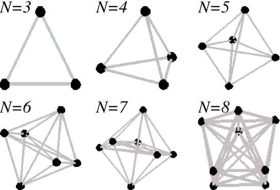
Figure 2: The configurations that maximize $F_{N}$ defined by (17) for identical Coulombian attractive particles.

However the sequence of improvements obtained this way seems to saturate up to $\alpha_{\infty}=2/9$:

$$\alpha_{3}=\alpha_{4}=\frac{1}{4}\geqslant\alpha_{5}\simeq.2432\geqslant\alpha_{6}\simeq.2414\geqslant\alpha_{7}\simeq.2382\geqslant\alpha_{8}\simeq.2366\geqslant\cdots\\ \cdots\geqslant\alpha_{30}\simeq.2266\cdots\geqslant\alpha_{\infty}=\frac{2}{9}\simeq.2222\;.$$ (28)

From the optimized configuration obtained with $N$ about several tens (see figure 3a), we can hopefully guess that the limit $N\to\infty$ leads to a continuous and uniform distribution of the particles on the same sphere. The continuous limit of $\sup_{\mathcal{Q}_{N}}F_{N}$ varies as $N^{3}$ with $N$. If, on the unit sphere $\mathcal{S}$, the $N$ particles get distributed uniformly with density $\sigma=N/4\pi$, the continuous limit of $\sup_{\mathcal{Q}_{N}}F_{N}$ is given by ($\mathrm{d}S_{i}$ is an infinitesimal portion of the sphere near the point $P_{i}$, $i=0,1,2$; see figure 3b)

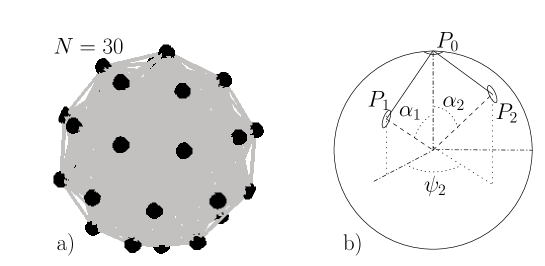
Figure 3: For large $N$, $F_{N}$ is maximized for a configuration where the $N$ points seems, numerically, to distribute uniformly on a sphere (with the well-know caveat concerning the ambiguity of such a notion [22]). Such an optimal configuration for $N=30$ is shown in a). The continuous limit of  $F_{N}/N^{3}$ when $N\to\infty$ can be computed with the help of figure b).

$$\sup_{\mathcal{Q}_{N}}F_{N} \!\sim\! \int_{\mathcal{S}}\sigma\,\mathrm{d}S_{0}\;\frac{1}{2}\int_{\mathcal{S}}\sigma\,\mathrm{d}S_{1}\int_{\mathcal{S}}\sigma\,\mathrm{d}S_{2}\,\cos(\widehat{P_{1},P_{0},P_{2}})\;;$$

$$\!\sim\! \frac{1}{2}\sigma^{3}\,8\pi^{2}\int_{0}^{\pi}\mathrm{d}\alpha_{1}\int_{0}^{\pi}\mathrm{d}\alpha_{2}\int_{0}^{2\pi}\mathrm{d}\psi_{2}\,\sin(\alpha_{1})\sin(\alpha_{2})\cos(\widehat{P_{1},P_{0},P_{2}}).$$

When $\cos(\widehat{P_{1},P_{0},P_{2}})=\frac{\mathbf{P_{0}P_{1}}}{||\mathbf{P_{0}P_{1}}||}\cdot\frac{\mathbf{P_{0}P_{2}}}{||\mathbf{P_{0}P_{2}}||}$ is expressed as a function of $\alpha_{1}$, $\alpha_{2}$ and $\psi_{2}$, we straightforwardly get $\sup_{\mathcal{Q}_{N}}F_{N}/N^{3}\sim_{N\to\infty}2/9=\alpha_{\infty}$. For infinite $N$, this last result supplement the upper bound given by (22) and we have

$$N\to\infty;\qquad-\frac{1}{18}\simeq-.0556\lesssim\ \frac{E_{0}}{N^{3}}\ \lesssim-.0542\;.$$ (29)

3.2 Three particles with one different from the two others

Without loss of generality, we can choose units where $e_{12}=e_{13}=e_{23}=-1$,  $m_{1}=m_{2}=1$, $m_{0}=m$. For $\textsc{d}=3$ the local energy (15) simplifies into

$$E_{\mathrm{loc}}^{[\varphi]}(q_{3})=-\frac{5m+1}{4(m+1)}-\frac{m}{2(m+1)}\left(\cos\theta_{1}+\cos\theta_{2}+\frac{2}{m+1}\cos\theta_{3}\right)\;.$$ (30)

The general study of appendix Appendix: Extrema for the three-body Coulombian problem applied for $(a_{1},a_{2},a_{3})=(1,1,\frac{2}{m+1})$ allows to get the following analytic bounds on $E_{0}$:

$$0\leqslant m \leqslant 1; \quad-\frac{1}{4}-\frac{m}{8}-\frac{m(m+2)}{(m+1)^{2}} \leqslant E_{0}\leqslant-\frac{1}{4}-\frac{m(2m+1)}{(m+1)^{2}}\;;$$ (31a)

$$1\leqslant m \leqslant 3; \quad-\frac{1}{4}-\frac{m}{8}-\frac{m(m+2)}{(m+1)^{2}} \leqslant E_{0}\leqslant-\frac{1}{4}-\frac{m(m+2)}{(m+1)^{2}}\;;$$ (31b)

$$3\leqslant m \quad-\frac{1}{4}-\frac{m(2m+1)}{(m+1)^{2}} \leqslant E_{0}\leqslant-\frac{1}{4}-\frac{m(m+2)}{(m+1)^{2}}\;.$$ ; (31c)

For $m\leqslant 3$, the lower bound on $E_{0}$ corresponds to a configuration where the particles make a non-degenerate isosceles triangle whose three angles are given by $\cos\theta_{1}=\cos\theta_{2}=(m+1)/4$ and $\cos\theta_{3}=1-(m+1)^{2}/8$. The other bounds correspond to configurations where the particles are aligned. For $m\gg 1$, the bounds saturates to $-9/4\lesssim E_{0}\lesssim-5/4$ which is quite rough compared to the numerical value $E_{0}>-1.8$ obtained for $m=20$ with the optimized variational method; yet it is better than the results given by the improved (Hall-Post) variational method [3, Table 2] with which it coincides for $m\leqslant 1$. For small $m$ both upper and lower bounds tend to the 2-body exact energy and provide acceptable bounds: For instance, when $m=0.05$, the differential method gives $-.34922\leqslant E_{0}\leqslant-.29989$ while the other ones [3, Table 2] give $-.59525\leqslant E_{0}$ (naive variational method) , $-.34922\leqslant E_{0}$ (improved variational method), $-.34666\leqslant E_{0}$ (optimized variational method) and $E_{0}\leqslant-.3375$ (variational with hyperspherical expansion up to $L=8$).

As already mentioned, the differential method, though being less precise for $N=3$ than the improved or hyperspherical variational approaches, has several advantages: it is much simpler, it provides analytic upper and lower bounds that furnish an explicit estimation of the errors and, at last but not least, can be easily extended to larger $N$ (see below) ; though possible in principle, the generalization of the improved variational method has not been done beyond $N=4$.

$m$	Naive	Hall-Post	Optimized	Variational	$E_{0}^{\mathrm{(d.m.)}}$	$\Delta E_{0}^{\mathrm{(d.m.)}}$	$E_{0}^{\mathrm{(d.m.)}}\mathop{-}\Delta E_{0}^{\mathrm{(d.m.)}}$
0.05	-0.59525	-0.34922	-0.34666	-0.3375	-0.3246	0.02467	-0.3492
0.1	-0.6818	-0.436055	-0.43434	-0.423465	-0.3926	0.04344	-0.4361
0.2	-0.8333	-0.58055	-0.58045	-0.55915	-0.5125	0.06806	-0.5806
0.5	-1.16667	-0.86805	-0.86705	-0.8242	-0.7813	0.08681	-0.8681
1	-1.5	-1.125	-1.125	-1.067	-1.0625	0.06250	-1.1250
2	-1.83333	-1.3889	-1.37135	-1.30225	-1.2639	0.12500	-1.3889
5	-2.16667	-1.8472	-1.61705	-1.53935	-1.5000	0.27778	-1.7778
10	-2.3182	-2.49175	-1.731	-1.6495	-1.6136	0.37190	-1.9855
20	-2.40475	-3.74775	-1.7972	-1.7134	-1.6786	0.43084	-2.1094

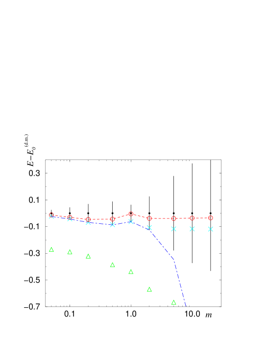
Figure 4: Estimations for the ground-state energy $E_{0}$ of an attractive Coulombian system made of three particles with masses $(m,1,1)$. Naive ($\triangle$), Hall-Post (also called improved, dashed-dotted link) and Optimized ($\times$) provide lower bounds on $E_{0}$ while Variational (open circles with a dashed link) provides an upper bound. The corresponding data are taken from[3]. In the graph, the value of $E_{0}^{\mathrm{(d.m.)}}$ has been subtracted. The error-bars are centered at zero (filled-circles) and have a width $2\Delta E_{0}^{\mathrm{(d.m.)}}$.

3.3 Several examples of four-body systems

The optimized variational method has been successfully proposed for $N=4$ in [4] for potentials with scaling-law behavior. For Coulombian interactions with a common coupling constant set to $-1$, tables and figures 5 and 6 compare the variational results to those obtained from the differential method when $\textsc{d}=3$. The same conclusion as in the previous section can be drawn and here are some examples of explicit analytic bounds that are obtained by partitioning $F_{4}$ in subclusters made of 3 particles:

Let us take $m_{1}=m_{2}=m_{3}=1$ and $m_{0}=m$. We have

$$0\leqslant m\leqslant 1;\quad-\frac{9}{8}-\frac{3m(m^{2}+6m+13)}{8(m+1)^{2}}\leqslant E_{0}\;;$$ (32a)

$$1\leqslant m\leqslant 2\sqrt{3}-1;\\ -\frac{9}{8}-\frac{3m(m^{2}+6m+13)}{8(m+1)^{2}}\leqslant E_{0}\leqslant-\frac{5m^{2}+13m+2}{2(m+1)^{2}}\;;$$ (32b)

$$2\sqrt{3}-1\leqslant m;\\ -\frac{9}{8}-\frac{3m(m^{2}+6m+13)}{8(m+1)^{2}}+\frac{3m(m+1-2\sqrt{3})^{2}}{8(m+1)^{2}}\leqslant E_{0}\leqslant-\frac{5m^{2}+13m+1}{2(m+1)^{2}}\;.$$ (32c)

The configuration that minimizes $E_{\mathrm{loc}}^{[\varphi]}(q_{4})$ given by (15) corresponds to a tetrahedron with an equilateral basis made by particles 1, 2 and 3. The three other faces, with particle $0$ at one vertex, are identical isosceles triangles, namely those which maximize (30) when $m\leqslant 3$. Such a tetrahedron can indeed be constructed provided the angles at particle $0$ are lower than $2\pi/3$ which requires $m\leqslant 2\sqrt{3}-1\simeq 2.464$. For $m\geqslant 2\sqrt{3}-1$, the configuration that minimizes $E_{\mathrm{loc}}^{[\varphi]}(q_{4})$ seems numerically to correspond to an equilateral triangle made by particles 1, 2 and 3 with particle $0$ at its center (the flat tetrahedron obtained when $m=2\sqrt{3}-1$). This simple configuration allows to conjecture the analytic lower bound in (32c). For $m\geqslant 1$, the upper bound is obtained when the four particles are aligned with the $0^{\mathrm{th}}$ at one extremity. For $m\leqslant 1$, I am not able to propose an analytic expression for the upper bound.

$m$	Naive	Hall-Post	Optimized	Variational	$E_{0}^{\mathrm{(d.m.)}}$	$\Delta E_{0}^{\mathrm{(d.m.)}}$	$E_{0}^{\mathrm{(d.m.)}}\mathop{-}\Delta E_{0}^{\mathrm{(d.m.)}}$
0.01	-2.29455	-1.17301	-1.17283	-1.108281	-1.10	0.07	-1.1730
0.1	-2.65909	-1.54679	-1.54167	-1.45802	-1.39	0.16	-1.5468
0.5	-3.75	-2.47917	-2.47618	-2.28857	-2.20	0.28	-2.4792
1	-4.5	-3	-3	-2.78762	-2.7500	0.2500	-3.0000
3	-5.625	-3.9375	-3.73167	-3.45553	-3.3024	0.6149	-3.9173
10	-6.3409	-6.48655	-4.20877	-3.90826	-3.6691	1.0575	-4.7266
100	-6.70545	-40.1395	-4.4673	-4.154310	-3.8412	1.3266	-5.1678
500	-6.741	-190.128	-4.49338	-4.17914	-3.8574	1.3545	-5.2119
$+\infty$	-6.75	$-\infty$	-4.5	-4.19259	-3.8615	1.3615	-5.2231

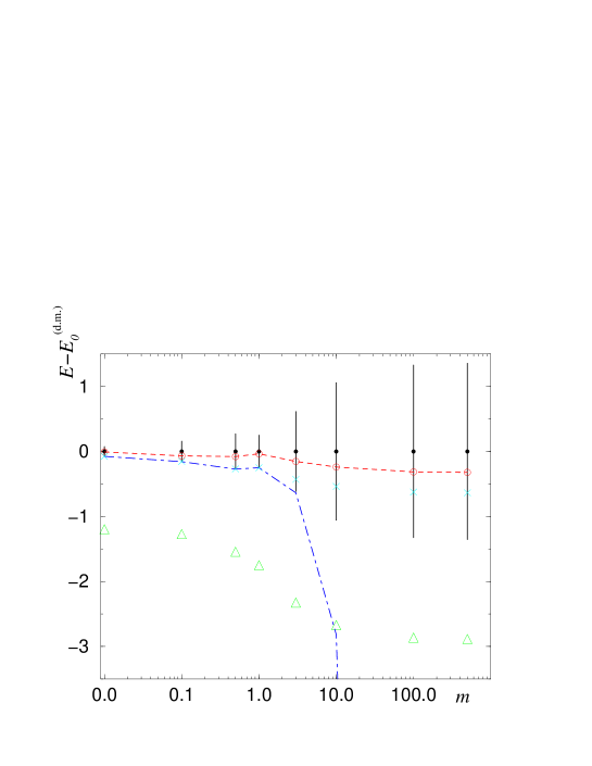
Figure 5: Same conventions as in figure 4 for an attractive Coulombian system made of four particles with masses $(m,1,1,1)$.

For $m_{2}=m_{3}=1$ and $m_{0}=m_{1}=m$, a tetrahedron that maximizes all the contributions of its faces simultaneously can be constructed for $m_{\star}^{-1}\leqslant m\leqslant m_{\star}\stackrel{{\scriptstyle\mathrm{def}}}{{=}}(-1+\sqrt{17}+\sqrt{14-2\sqrt{17}})/2$. Two identical faces (see figure  7) corresponding to particles with masses $(1,1,m)$ have their three angles given by $\cos\theta_{1}=\cos\theta_{2}=(m+1)/4$ and $\cos\theta_{3}=1-(m+1)^{2}/8$. The angles $(\theta_{1}^{\prime}=\theta_{2}^{\prime},\theta_{3}^{\prime})$ of the two other faces corresponding to particles with masses $(m,m,1)$ are obtained replacing $m$ by $m^{-1}$ in the previous expressions. For $1/3\leqslant m\leqslant 3$ such faces can indeed be constructed but the pairs of identical faces can be put together to construct one tetrahedron provided only that $\theta_{3}\leqslant 2\theta_{1}^{\prime}$. This last condition leads to $m^{4}+2m^{3}-14m^{2}+2m+1\leqslant 0$. $m_{\star}$ and $m_{\star}^{-1}$ are the two positive roots of the four-degree-polynomial, the two others being negative. We get

$$m_{\star}^{-1}\simeq.3622\leqslant m\leqslant m_{\star}\simeq 2.7609;\quad-\frac{m^{2}+10m+1}{2(m+1)}\leqslant E_{0}\;.$$ (33)

$m$	Naive	Hall-Post	Optimized	Variational	$E_{0}^{\mathrm{(d.m.)}}$	$\Delta E_{0}^{\mathrm{(d.m.)}}$	$E_{0}^{\mathrm{(d.m.)}}\mathop{-}\Delta E_{0}^{\mathrm{(d.m.)}}$
0.001	-0.756745	-0.504495	-0.25557	-0.25492	-0.2543	0.0021	-0.2564
0.002	-0.763475	-0.508985	-0.26114	-0.25985	-0.2587	0.0042	-0.2629
0.005	-0.7836	-0.5224	-0.277805	-0.2746	-0.2717	0.0104	-0.2820
0.01	-0.816905	-0.544605	-0.305465	-0.32403	-0.2931	0.0204	-0.3135
0.05	-1.07322	-0.715475	-0.519635	-0.50503	-0.4581	0.0913	-0.5494
0.1	-1.37045	-0.913635	-0.76439	-0.7308	-0.6492	0.1594	-0.8086
0.2	-1.9	-1.26666	-1.17921	-1.10975	-0.9893	0.2448	-1.234
0.5	-3.125	-2.08333	-2.06426	-1.91867	-1.7847	0.2986	-2.0833†
0.8	-4.01666	-2.67778	-2.67552	-2.48094	-2.4034	0.2744	-2.6778†
1	-4.5	-3	-3	-2.78736	-2.7500	0.2500	-3.0000†

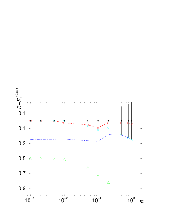
Figure 6: Same conventions as in figure 4 for an attractive Coulombian system made of four particles with masses $(m,m,1,1)$. Numbers signaled with a ^† are the lower bounds (33).

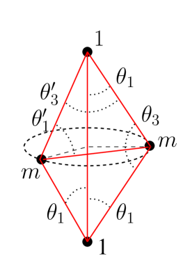
Figure 7: For a special range of $m$, a four-body configuration with masses $(m,m,1,1)$ that minimizes the local energy can be constructed from the optimal configurations of each of its three-body subsystems.

3.4 Arbitrary number of identical particles plus one different from the others

As we have already seen for identical particles, the possibility of partitioning the local energy in contributions involving more than two particles allow to get some bounds on the ground-state energy of systems made of an arbitrary number $N$ of particles. For $N\geqslant 5$, this is beyond the scope of the existing optimized variational methods. To see one more last example, let us generalize both cases of sections 3.1 and 3.2 and consider a system made of one particle with mass $m_{0}=m$ and $N-1$ identical particles of mass $m_{1}=\cdots=m_{N-1}=1$. All the identical particles interact with the same coupling constants $e_{ij}=-1$ and the $0^{\mathrm{th}}$ interact with $e_{0,i}=-g^{2}$. The local energy is given by (15) as

$$E_{\mathrm{loc}}^{[\varphi]}(q_{N})=-\frac{1}{(\textsc{d}-1)^{2}}\Bigg{\{}\frac{2mg^{4}}{m+1}(N-1)+\frac{1}{2}(N-1)(N-2)+F_{N-1}(q_{N-1})\\ +a(m^{-1})\sum^{N-1}_{\begin{subarray}{c}i,j=1\\ i<j\end{subarray}}\left[\cos(\widehat{0ij})+\cos(\widehat{0ji})+a(m)\cos(\widehat{i0j})\right]\Bigg{\}}$$ (34)

where now $q_{N-1}$ stands for the configuration of the $N-1$ identical particles. $a(m)\stackrel{{\scriptstyle\mathrm{def}}}{{=}}2g^{2}/(m+1)$. By simultaneously bounding the contributions of the triangles that include the $0^{\mathrm{th}}$ particle and the contribution of the remaining cluster of the identical particles, we immediately have analytic expressions for bounds on $E_{0}$. For instance the lower bound is given by

$$E_{0}\geqslant-\frac{1}{(\textsc{d}-1)^{2}}\Bigg{\{}\frac{2mg^{4}}{m+1}(N-1)+\frac{1}{2}(N-1)(N-2)+\sup_{\mathcal{Q}_{N-1}}F_{N-1}\\ +\frac{1}{2}\,a(m^{-1})(N-1)(N-2)F_{3}^{\mathrm{max}}\big{(}1,1,a(m)\big{)}\Bigg{\}}$$ (35)

where $F_{3}^{\mathrm{max}}$ is given by (62) and $\sup_{\mathcal{Q}_{N-1}}F_{N-1}$ has been explicitly estimated in section 3.1.

4 Arbitrary two-body interaction

4.1 Behavior at large distances

Considering attractive Coulombian interactions is relevant for heavy quarks models at short distances but, of course, other kinds of effective potentials are required in most models. Since in general no analytic expressions are known for the two-body ground-state energies $\epsilon_{ij}$, no method is expected to provide explicit non-trivial bounds on $E_{0}$. However, if one has some experimental clues about $\epsilon_{ij}$ (by measuring 2-body masses or dissociation energies) or numerical estimates as well, it is always interesting to obtain some relations between the $\epsilon$’s and the ground-state energies of larger systems. As mentioned in the introduction, this have been achieved in [2] for $N=3$ and in [4] for $N=4$ when the interactions are of the form $v_{ij}(r)\propto\mathrm{sign}(\beta)r^{\beta}$.

For $\beta>0$, the semiclassical argument given at the end of section 2 shows that (13) is expected to be unbounded; then (4) gives no information. If we want to take the advantage of the simple form (13) (that is, to keep the choice (9) with (11) for the test functions), we have to work with finite range potentials. When at large distances, the potential is still confining ($\beta=2$ for harmonic forces or $\beta=1$ for interquark force in quantum chromodynamics [9] and [5, for an up-to-date review]), some different ansatz for $\varphi$ must be constructed in order to eliminate the singular behavior of the $v_{ij}$’s at infinite distances. Actually, the Coulombian case considered in the previous section can be seen as an example of a problem where simple poles at finite distances can be eliminated. Anyway, in many situations, the 2-body ground-state is expected to depend on the behavior of the potential at large distances by exponentially small terms only. If, in the integral (3), we decide to keep only those configurations $q_{N}$ whose size remains in a physical domain bounded by a cut-off length $\Lambda$, then we expect to make an exponentially small error on the estimates of $E_{0}$; this is due to the exponential decay of $\Phi_{0}$ when two or more particles separate off. Like the $\epsilon_{ij}$’s, $\Lambda$ is typically obtained from a 2-body dynamics but its precise value is irrelevant if the extremal values of the local energy do not depend on it. It is precisely the case of the Coulombian interactions (more exactly, interactions that can be modeled by Coulombian potential at the energy scale where the ground-state exists) for which the local energy (15) is invariant under dilations.

Since, in the present section, we just want to sketch some main guidelines without working through the details neither being exhaustive, we will consider only the cases where

$$v(r)\underset{r\to+\infty}{\longrightarrow}0\;.$$ (36)

4.2 Fitting the 2-body ground-state wavefunction

What is new, here, is that the differential method allows us to choose directly the 2-body ground-state wave-functions, or rather their logarithms $S_{ij}$. Once some numerical estimate of $\epsilon_{ij}$ is obtained in one way or another, we can completely bypass the problem of modeling the 2-body potential uniformely. Being free of any integration, the differential method can deal with rather complicated, and therefore rather realistic two-body test functions. An explicit choice of $S_{ij}$’s provides an explicit form for the local energy (13).

It frequently happens that we know from experiments the behavior of the two-body potential in some specific regimes (most generally at short and large distances) but not uniformly. We can therefore, in each of these regimes, tentatively obtain, with the help of the differential equation (11), the local functional form of the two-body ground-state wave-function. Matching these local solutions together, and then dealing with quite complicated global expression for $S$ and $v$, do not represent a serious obstacle for the computation of (13).

To be a little less speculative, let us consider $N$ identical particles with unit mass, interacting with a two-body radial potential $v(r)$ such that $v(r)\to 0$ when $r\to\infty$ and

$$v(r)\underset{r\to 0^{+}}{\longrightarrow}v_{0}\,r^{\beta}$$ (37)

for some $v_{0}$ and with considering only one case, say $\beta>0$. The two-body stationary Schrödinger equation (11) becomes

$$-\left(\frac{\mathrm{d}^{2}}{\mathrm{d}r^{2}}+\frac{\textsc{d}-1}{r}\frac{\mathrm{d}}{\mathrm{d}r}\right)\phi+v\phi=\epsilon_{0}\phi$$ (38)

where $\epsilon_{0}<0$ will denote an estimate of the two-body ground-state energy; it can be considered as another parameter that should fit the experiments involving two bodies. Let us guess the behavior of $S(r)\stackrel{{\scriptstyle\mathrm{def}}}{{=}}\ln\phi(r)$ at short distances by writing for $\sigma\neq-1$:

$$S(r)\underset{r\to 0^{+}}{\longrightarrow}\frac{s_{0}}{\sigma+1}\,r^{\sigma+1}\;.$$ (39)

Identifying the leading orders after having reported (39) in (38), we necessarily get (for $\textsc{d}>1$) $\sigma=1$ and $s_{0}=-\epsilon_{0}/\textsc{d}$. The next term in the development of $S$ can also be determined. For $0<\beta<2$, it depends only on the leading term (37) and we have

$$S(r)\underset{r\to 0^{+}}{\longrightarrow}-\frac{\epsilon_{0}}{2d}\,r^{2}+\frac{v_{0}}{(\textsc{d}+\beta)(2+\beta)}\,r^{2+\beta}+o(r^{2+\beta})\;.$$ (40)

This local asymptotic series must be matched with the semiclassical behavior at large $r$

$$S(r)\underset{r\to+\infty}{\longrightarrow}-\sqrt{-\epsilon_{0}}\,r$$ (41)

since we have supposed (36). The additive constant in $S$ is irrelevant since the local energy does not depend on the normalization of $\phi$. A simple choice that ensures the local energy to remain uniformly bounded is to take for $S^{\prime}$ a fraction like

$$S^{\prime}(r)=\frac{-\frac{\epsilon_{0}}{\textsc{d}}\,r+\frac{v_{0}}{\textsc{d}+\beta}\,r^{1+\beta}-\sqrt{-\epsilon_{0}}\,r^{1+2\beta}}{1+r^{1+2\beta}}\;.$$ (42)

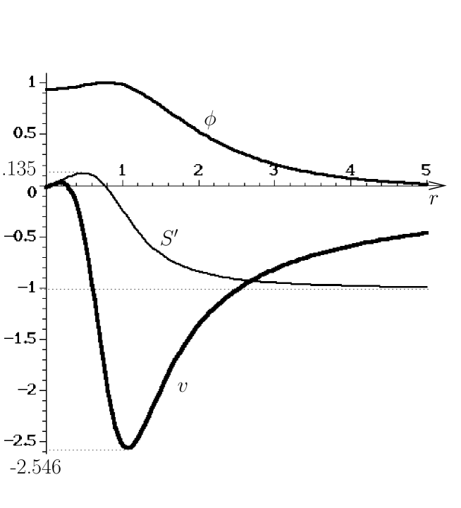
Figure 8: $\textsc{d}=3$, $\epsilon_{0}=-1$, $v_{0}=1$, $\beta=1.5$, the function $S^{\prime}$ given by (42) is plotted as well as the corresponding wavefunction $\phi=\exp{S}$ which is the ground-state of the potential $v$ for energy $\epsilon_{0}$. The latter can be reconstructed from $\phi$ with the Schrödinger equation.

Figure 8 show the corresponding $\phi$ for an arbitrary choice of parameters together with the corresponding $v$ whose complicated analytic expression on $[0,+\infty[$ is not needed.

4.3 Crude bounds

From equation (13), an immediate upper bound on $E_{0}$ is given by:

$$\frac{1}{2}N(N-1)\,\epsilon_{0}-\frac{1}{2}N(N-1)(N-2)\,\sigma^{2}\leqslant E_{0}\\ \leqslant\frac{1}{2}N(N-1)\,\epsilon_{0}+\frac{1}{2}N(N-1)(N-2)\,\sigma^{2}$$ (43)

where

$$\sigma\stackrel{{\scriptstyle\mathrm{def}}}{{=}}\sup_{[0,+\infty[}|S^{\prime}|\;.$$ (44)

Because the constraints between the angles $\widehat{j,i,k}$ are not taken into account, these inequalities are expected to be rather rough and their quality deteriorate for large $N$: when positive, the upper bound becomes irrelevant since we already know that $E_{0}\leqslant 0$. Indeed, the decreasing of the $\sigma^{2}$ term with $N$ does not guarantee that the lower bound is better than the Hall-Post bound $N(N-1)\tilde{\epsilon}_{0}/2$ or even than the naive one $N(N-1)\tilde{\tilde{\epsilon}}_{0}/2$ [4, § 2.1 and 2.2] where $\tilde{\tilde{\epsilon}}_{0}$ (resp. $\tilde{\epsilon}_{0}$ and $\epsilon_{0}$) is the ground-state energy for a particle of mass $(N-1)/2$ (resp. $N/4$ and 1/2) in the central potential $v$ (recall $\tilde{\tilde{\epsilon}}_{0}<\tilde{\epsilon}_{0}<\epsilon_{0}$).

4.4 Reduction to a finite number of Coulombian cases

In fact, we can find some bounds of (13) by reducing the problem to a finite number of Coulombian-like cases, that is, where the function to be bound involves constant factors in front of the cosine (compare (15) to (13)). To see this, split the coordinates $q_{N}$ into a scaling factor $\lambda\geqslant 0$ and some angle variables $\theta$ among which $(N-1)\textsc{d}-1$ are independent. Each distance writes $r_{ij}=\lambda\rho_{ij}(\theta)$ where the $\rho_{ij}$’s are functions that do not depend on the global size of the configuration but on its shape only. Now, from (13), we define (recall $m_{i}=1$)

$$G_{N}(q_{N})\stackrel{{\scriptstyle\mathrm{def}}}{{=}}\sum_{(\widehat{j,i,k})}S^{\prime}(r_{ij})S^{\prime}(r_{ik})\cos(\widehat{j,i,k})$$ (45)

and we have

$$\inf_{q_{N}}\big{(}G_{N}(q_{N})\big{)}=\inf_{\theta}\big{(}\tilde{G}_{N}(\theta)\big{)}$$ (46)

where

$$\tilde{G}_{N}(\theta)=\inf_{\lambda}\sum_{(\widehat{j,i,k})}S^{\prime}[\lambda\rho_{ij}(\theta)]\,S^{\prime}[\lambda\rho_{ik}(\theta)]\cos(\widehat{j,i,k})\;.$$ (47)

Analogous relations are obtained for the maxima. For fixed $\theta$, when $\lambda$ varies from $0$ to $+\infty$, the map $\lambda\mapsto\big{(}S^{\prime}[\lambda\rho_{ij}(\theta)]\big{)}_{0\leqslant i<j\leqslant N-1}$ defines a curve $\mathcal{C}_{\theta}$ in a $n$-dimensional space with $n=N(N-1)/2$. $\mathcal{C}_{\theta}$ is bounded if $S^{\prime}$ is bounded. More precisely, $\mathcal{C}_{\theta}$ is inside the $n$-dimensional hypercube $\mathcal{B}\stackrel{{\scriptstyle\mathrm{def}}}{{=}}[\sigma_{\mathrm{min}},\sigma_{\mathrm{max}}]^{n}$ where

$$\sigma_{\mathrm{min}}\stackrel{{\scriptstyle\mathrm{def}}}{{=}}\inf_{[0,+\infty[}S^{\prime}$$ (48a)

and

$$\sigma_{\mathrm{max}}\stackrel{{\scriptstyle\mathrm{def}}}{{=}}\sup_{[0,+\infty[}S^{\prime}\,.$$ (48b)

If $S^{\prime}$ has the form shown in figure 8, $\mathcal{C}_{\theta}$ starts at the origin ($S^{\prime}(0)=0$) and ends at the point $(-1,\dots,-1)$. Taking all the points in $\mathcal{B}$ rather than the points of $\mathcal{C}_{\theta}$ leads to a lower bound of $\tilde{G}_{N}$:

$$\inf_{\vec{s}\in\mathcal{B}}\sum_{(\widehat{j,i,k})}s_{ij}\,s_{ik}\cos(\widehat{j,i,k})\leqslant\tilde{G}_{N}(\theta)$$ (49)

where $\vec{s}=(s_{ij})_{0\leqslant i<j\leqslant N-1}$. Now, whatever the values of the cosines may be, the quadratic function in $\vec{s}$ appearing in the left-hand side of (49) reaches its minimum at a vertex of $\mathcal{B}$. Let us denote by $\mathcal{V}$, the finite set of the $2^{n}$ vertices $\vec{s}$ of $\mathcal{B}$ (i.e. for all $\vec{s}$ in $\mathcal{V}$, each $s_{ij}$ is either $\sigma_{\mathrm{min}}$ or $\sigma_{\mathrm{max}}$). We have

$$\inf_{\vec{s}\in\mathcal{V}}\big{[}\inf_{\theta}\big{(}F^{(\vec{s}\,)}_{N}(\theta)\big{)}\big{]}\leqslant\inf_{q_{N}}\big{(}G_{N}(q_{N})\big{)}\;.$$ (50)

where

$$F^{(\vec{s}\,)}_{N}(\theta)\stackrel{{\scriptstyle\mathrm{def}}}{{=}}\sum_{(\widehat{j,i,k})}s_{ij}s_{ik}\cos(\widehat{j,i,k})\;.$$ (51)

In fact, what we have done by obtaining the left-hand side of (50) is to make the values of $S^{\prime}(r_{ij})$ independent from those of $\theta$. It follows that the inequality (50) will be strict if the value of $\vec{s}$ at the minimizing vertex are incompatible with the geometrical constraints on the configuration of the $N$ points. We will illustrate this point in the next subsection. We have obtained

$$E_{0}\leqslant\frac{1}{2}N(N-1)\epsilon_{0}-\inf_{\vec{s}\in\mathcal{V}}\big{[}\inf_{\theta}\big{(}F^{(\vec{s}\,)}_{N}(\theta)\big{)}\big{]}\;.$$ (52a)

and similarly

$$\frac{1}{2}N(N-1)\epsilon_{0}-\sup_{\vec{s}\in\mathcal{V}}\big{[}\sup_{\theta}\big{(}F^{(\vec{s}\,)}_{N}(\theta)\big{)}\big{]}\leqslant E_{0}\;.$$ (52b)

The function $F^{(\vec{s}\,)}_{N}(\theta)$ has the same form as the second sum of the right-hand of $\eqref{eq:ElocNbodyCoulomb}$. Therefore, the computation of the bounds in (52) is equivalent to a finite number of Coulombian problems (with not necessarily attractive interactions since the sign of $s_{ij}$ may change) where we must consider all the possible $\vec{s}$ whose components are either $\sigma_{\mathrm{min}}$ or $\sigma_{\mathrm{max}}$.

4.5 Three bodies

As we have seen in section 3, even in the purely attractive Coulombian cases, an analytic expression of the extrema of $F_{N}$ is not known in general. Anyway, one can always group in clusters the terms involved in (51) like in (24), then use inequalities like (25) and reduce the number of particles. Let us then consider $N=3$. It can be shown that

$$\inf_{\vec{s}\in\mathcal{V}}\big{[}\inf_{\theta}\big{(}F^{(\vec{s}\,)}_{3}(\theta)\big{)}\big{]}=2\sigma_{\mathrm{min}}\sigma_{\mathrm{max}}-\sigma^{2}$$ (53)

with definitions (44) and (48). $\inf_{\theta}F^{(\vec{s}\,)}_{3}(\theta)$ is obtained for an aligned configuration which is generically incompatible with $\vec{s}$ being a vertex of the cube $[\sigma_{\mathrm{min}},\sigma_{\mathrm{max}}]^{3}$. For instance, suppose that $S^{\prime}$ has the shape depicted in figure 8 where $\sigma=-\sigma_{\mathrm{min}}>\sigma_{\mathrm{max}}>0$; the value $2\sigma_{\mathrm{min}}\sigma_{\mathrm{max}}-\sigma_{\mathrm{min}}^{2}$ is obtained for $\vec{s}=(s_{01},s_{02},s_{12})=(\sigma_{\mathrm{min}},\sigma_{\mathrm{min}},\sigma_{\mathrm{max}})$ and should be realized for $r_{01}\gg 1$, $r_{02}\gg 1$ and $r_{12}\simeq r_{\mathrm{max}}$ (the unique finite distance at which $S^{\prime\prime}$ vanishes); but this is incompatible with the alignment condition $\cos(\widehat{1,0,2})=-1$ where particle $0$ is in between the two others which implies $r_{12}=r_{01}+r_{02}$. The inequality (50) is therefore strongly strict. It can be improved by reducing the size of the cube $\mathcal{B}$ to make its minimizing vertices compatible with the aligned configuration. It can be shown that for $S^{\prime}$ of the form shown in figure 8, we have

$$2\sigma_{\mathrm{max}}S^{\prime}(2r_{0})-\sigma_{\mathrm{max}}^{2}\leqslant\inf_{q_{3}}\big{(}G_{3}(q_{3})\big{)}$$ (54)

where $r_{0}$ is the unique strictly positive distance where $S^{\prime}$ vanishes. Even though the inequality is still strict because $r_{12}=2r_{0}\neq r_{01}+r_{02}=2r_{\mathrm{max}}$ in general, the bound is much better than (53). For instance, if we take the value of the parameters corresponding to figure 8 we have

$$2\sigma_{\mathrm{min}}\sigma_{\mathrm{max}}-\sigma_{\mathrm{min}}^{2}\simeq-1.2705<2\sigma_{\mathrm{max}}S^{\prime}(2r_{0})-\sigma_{\mathrm{max}}^{2}\simeq-.205\;.$$ (55)

to be compared with the result of the numerical minimization of $G_{3}$

$$\inf_{q_{3}}\big{(}G_{3}(q_{3})\big{)}\simeq-.1150\;.$$ (56)

obtained for the aligned configuration where $r_{01}=r_{02}=r_{12}/2\simeq.6107$.

The other bound

$$\sup_{q_{3}}\big{(}G_{3}(q_{3})\big{)}=\sup_{\vec{s}\in\mathcal{V}}\big{[}\sup_{\theta}\big{(}F^{(\vec{s}\,)}_{3}(\theta)\big{)}\big{]}=\frac{3}{2}\,\sigma^{2}$$ (57)

is actually obtained at the vertex $\vec{s}=(\sigma,\sigma,\sigma)$ for an equilateral configuration where the common distance $r_{01}=r_{02}=r_{12}$ is where $|S^{\prime}|$ reaches its maximum. For $S^{\prime}$ like in figure 8, it corresponds to a very large triangle ($r_{01}\gg 1$) where $\sigma\simeq 1$. For $\textsc{d}=3$, $\epsilon_{0}=-1$, $v_{0}=1$, $\beta=1.5$, from (50) and results (56), (57), the inequalities (52) give

$$-3-3/2=-4.5\leqslant E_{0}\leqslant-3+.1150=-2.885$$ (58)

corresponding to a relative error of $\Delta E_{0}^{\mathrm{(d.m.)}}/E_{0}^{\mathrm{(d.m.)}}\simeq 22\%$. This not really impressive (again we emphasize that we are not looking for numerical performance at this stage of development of the differential method) but can be seen as an encouraging starting point since the interactions involved so far in the three-body system are highly not trivial. It would have required much more numerical work to obtain a rigorous window for $E_{0}$ with variational methods (specially a lower bound since the potential considered here does not follow a power-law behavior).

5 Conclusion

The differential method appears to offer a completely new strategy for estimating a ground-state energy. For many-body systems, we have seen on several examples how this approach can be fruitful. For attractive Coulombian particles, it can compete with existing others methods (that are based on the variational principle) on several levels: it provides upper and lower bounds with comparable numerical precision, its simplicity renders the analytic calculations tractable even for large $N$ and/or allows a low cost of numerical computation. Beyond purely Coulombian systems, the differential method, being so general, offers a remarkable flexibility. As have been sketched in the previous section, one can deal with systems where interactions can be very rich (possibly short-ranged with an a priori cut-off); several regimes which are valid at different scales can be implemented at once. There is some hope that future works successfully apply the differential methods for proper realistic potentials.

Unfortunately, I have not been able to generalize the differential method to fermionic systems where the ground-state spatial wave-function is antisymmetric. In such cases, the presence of non-trivial nodal lines [6] breaks down the proof of inequalities (4).

There is a lot of work to be done regarding a systematic improvement of the bounds, once some finite ones have been found with a $\varphi$ given at first attempt. In this paper, we have not considered some free parameters on which a (family) of test functions, say $\varphi_{\zeta}$, may depend. As shown for a one-dimensional system [15], the locality of the differential method may require a very few number of $\lambda$’s at each optimization step (unlike for the variational test functions) for obtaining substantial improvements of the bounds by calculating, say $\sup_{\zeta}\big{[}\inf_{q}\big{(}E_{\mathrm{loc}}^{[\varphi_{\zeta}]}(q)\big{)}\big{]}$. A precise proof that this approach is efficient for several dimensions remains an open interesting problem.

I thank Jean-Marc Richard for a critical reading of the first proof of this manuscript and acknowledge the generous hospitality of Dominique Delande and Benoît Grémaud of the group “Dynamique des systèmes coulombiens” at the Laboratoire Kastler-Brossel.

Appendix: Extrema for the three-body Coulombian problem

For the three-body Coulombian problem, as can be seen from the second sum in the right-hand side of (15), we must find

$$F_{3}^{\mathrm{max}}(a_{1},a_{2},a_{3})\stackrel{{\scriptstyle\mathrm{def}}}{{=}}\sup_{\mathrm{triangles}}[a_{1}\cos\theta_{1}+a_{2}\cos\theta_{2}+a_{3}\cos\theta_{3}]$$ (59)

and

$$F_{3}^{\mathrm{min}}(a_{1},a_{2},a_{3})\stackrel{{\scriptstyle\mathrm{def}}}{{=}}\inf_{\mathrm{triangles}}[a_{1}\cos\theta_{1}+a_{2}\cos\theta_{2}+a_{3}\cos\theta_{3}]$$ (60)

where the $\theta$’s are the angles at the three vertices of the triangle made of the three particles. The $a$’s are some real parameters that depend on the masses and the coupling constants. Let us define

$$f(a_{1},a_{2},a_{3})\stackrel{{\scriptstyle\mathrm{def}}}{{=}}\frac{1}{2}\left(\frac{a_{1}a_{2}}{a_{3}}+\frac{a_{1}a_{3}}{a_{2}}+\frac{a_{2}a_{3}}{a_{1}}\right)\;,$$ (61)

then we have

$$F_{3}^{\begin{subarray}{c}\mathrm{max}\\ \mathrm{min}\end{subarray}}(a_{1},a_{2},a_{3})=\begin{subarray}{c}\mathrm{max}\\ {\mathrm{min}}\end{subarray}\{a_{1}+a_{2}-a_{3},a_{1}-a_{2}+a_{3},-a_{1}+a_{2}+a_{3},f(a_{1},a_{2},a_{3})\}$$ (62)

$f$ is considered in the list (62) if and only if the following three conditions are satisfied simultaneously

$$\frac{1}{2}\left|\frac{a_{2}}{a_{3}}+\frac{a_{3}}{a_{2}}-\frac{a_{2}a_{3}}{a_{1}^{2}}\right|\leqslant 1\;;\frac{1}{2}\left|\frac{a_{1}}{a_{2}}+\frac{a_{2}}{a_{1}}-\frac{a_{1}a_{2}}{a_{3}^{2}}\right|\leqslant 1\;;\frac{1}{2}\left|\frac{a_{3}}{a_{1}}+\frac{a_{1}}{a_{3}}-\frac{a_{1}a_{3}}{a_{2}^{2}}\right|\leqslant 1\;.$$ (63)

Here is the proof: We will restrict the values of the $\theta$’s to $[0,\pi]$ and the constraint $\theta_{1}+\theta_{2}+\theta_{3}=\pi$ is implemented by the Lagrange multiplier method. We are led to extremalise the function $G_{3}(\theta_{1},\theta_{2},\theta_{3})\stackrel{{\scriptstyle\mathrm{def}}}{{=}}a_{1}\cos\theta_{1}+a_{2}\cos\theta_{2}+a_{3}\cos\theta_{3}+\ell(\theta_{1}+\theta_{2}+\theta_{3}-\pi)$ for unconstrained $(\theta_{1},\theta_{2},\theta_{3})\in[0,\pi]^{3}$, $\ell$ being the Lagrange multiplier. The three conditions $\partial_{\theta_{i}}G_{3}=0$ for $i=1,2,3$ lead to $\ell=a_{1}\sin\theta_{1}=a_{2}\sin\theta_{2}=a_{3}\sin\theta_{3}$. The case $\ell=0$ corresponds to the alignment of the three particles and gives the three first values in the list (62) corresponding to $(\theta_{1},\theta_{2},\theta_{3})=(0,0,\pi)$ and its circular permutations.

Taking into account the constraint on the angles, we have $\ell=a_{3}\sin\theta_{3}=a_{3}\sin\theta_{1}\cos\theta_{2}+a_{3}\sin\theta_{2}\cos\theta_{1}=\ell(a_{3}\cos\theta_{2}/a_{1}+a_{3}\cos\theta_{1}/a_{2})$. Therefore when $\ell\neq 0$, we find $a_{1}\cos\theta_{1}+a_{2}\cos\theta_{2}=a_{1}a_{2}/a_{3}$ as well as the other relations that are obtained by circular permutations of the indices. From the decomposition $F_{3}=\frac{1}{2}(a_{1}\cos\theta_{1}+a_{2}\cos\theta_{2})+\frac{1}{2}(a_{2}\cos\theta_{2}+a_{3}\cos\theta_{3})+\frac{1}{2}(a_{1}\cos\theta_{1}+a_{3}\cos\theta_{3})$, we obtain the value (61) that must be considered in (62) if and only if there exists some $\theta$’s such that

$$a_{1}\sin\theta_{1}=a_{2}\sin\theta_{2}=a_{3}\sin\theta_{3}\quad\mathrm{and}\quad\theta_{1}+\theta_{2}+\theta_{3}=\pi\;.$$ (64)

Solving these three equations leads to the values for the three $|\cos\theta_{i}|$ that are precisely given by the left-hand sides of the inequalities (63).

References

- [1] J.-L. Basdevant, A. Martin, and J.-M. Richard. Improved bounds on many-body Hamiltonians. i. self-gravitating bosons. Nuclear Phys. B, 343(1):60–68, 1990.
- [2] J.-L. Basdevant, A. Martin, and J.-M. Richard. Improved bounds on many-body Hamiltonians. ii. baryons from mesons in the quark model. Nuclear Phys. B, 343(1):69–85, 1990.
- [3] J.-L. Basdevant, A. Martin, J.-M. Richard, and T. T. Wu. Optimized lower bounds in the three-body problem. Nuclear Phys. B, 393:111–125, 1993.
- [4] A. Benslama, A. Metatla, A. Bachkhaznadji, S. R. Zouzou, A. Krikeb, J.-L. Basdevant, J.-M. Richard, and T. T. Wu. Optimized lower bound for four-body Hamiltonians. Few-Body Systems, 24(1):39–54, 1998.
- [5] N. Brambilla et al. Heavy quarkonium physics. hep-ph/0412158, 2004.
- [6] D. M. Ceperley. Fermion nodes. J. Statist. Phys., 63(5/6):1237–1267, 1991.
- [7] Francisco M. Fernández, Q. Ma, and R. H. Tipping. Eigenvalues of the Schrödinger equation via the Riccati-Padé method. Phys. Rev. A (3), 40(11):6149–6153, 1989.
- [8] Michael E. Fisher and David Ruelle. The stability of many-particle systems. J. Math. Phys., 7(2):260–270, 1966.
- [9] Aaron K. Grant, Jonathan L. Rosner, and Eric Rynes. An updated description of quarkonium by power-law potentials. Phys. Rev. D (3), 47(5):1981–1987, 1993.
- [10] Carlos R Handy and Daniel Bessis. Rapidly convergent lower bounds for the Schrödinger-equation ground-state energy. Phys. Rev. Lett., 55(9):931–934, 1985.
- [11] Gregory Jaczko and Loyal Durand. Understanding the success of nonrelativistic potential models for relativistic quark-antiquark bound states. Phys. Rev. D (3), 58(11):114017, 1998.
- [12] A. Lenard and Freeman J. Dyson. Stability of matter. i. J. Math. Phys., 8(3):423–434, 1967.
- [13] Jean-Marc Lévy-Leblond. Nonsaturation of gravitational forces. J. Math. Phys., 10(5):806–812, 1969.
- [14] V. P. Maslov and M. V. Fedoriuk. Semi-Classical Approximation in Quantum Mechanics, volume 7 of Mathematical physics and applied mathematics. D. Reidel publishing company, Dordrecht, 1981.
- [15] Amaury Mouchet. A differential method for bounding the ground state energy. J. Phys. A, 38:1039–1047, 2005.
- [16] Amaury Mouchet. Upper and lower bounds for an eigenvalue associated with a positive eigenvector. math.SP/0505541, 2005.
- [17] S. Nussinov. Baryon-meson mass inequality. Phys. Rev. Lett., 51(23):2081–2084, 1983.
- [18] Bodmer A. R. and Shamsher Ali. A self-consistent two-body method for three-body systems and the hypernucleus . Nuclear Phys., 54:657–682, 1964.
- [19] Michael Reed and Barry Simon. Analysis of operators, volume 4 of Methods of modern mathematical physics. Academic Press, New York, 1978.
- [20] Jean-Marc Richard. Few-body problems in hadron spectroscopy. Nuclear Phys. A, 689:235–246, 2001.
- [21] Jean-Marc Richard. Borromean binding. nucl-th/0305076, 2003.
- [22] E. B. Saff and A. B. Kuijlaars. Distributing many points on a sphere. Math. Intelligencer, 19(1):5–11, 1997.
- [23] Peter Van Dyke and Robert Folk. Two-body equations for four-nucleon problems. Phys. Rev., 178(4):1537–1542, 1969.