Extraction of scattering lengths from final-state interactions

Abstract

A recently proposed method based on dispersion theory, that allows to extract the scattering length of a hadronic two-body system from corresponding final-state interactions, is generalized to the situation where the Coulomb interaction is present. The steps required in a concrete practical application are discussed in detail. In addition a thorough examination of the accuracy of the proposed method is presented and a comparison is made with results achieved with other methods like the Jost-function approach based on the effective-range approximation. Deficiencies of the latter method are pointed out. The reliability of the dispersion theory method for extracting also the effective range is investigated.

I Introduction

The scattering length provides not only an important measure for the strength of the interaction in a specific hadronic two-body system Joach but often allows to draw further more general and thus even more interesting conclusions. For example in the case of the proton-proton and neutron-neutron systems the corresponding scattering lengths in the ${}^{1}S_{0}$ partial wave provide a very sensitive test of charge symmetry in the strong interaction Miller . SU(3) symmetry can be tested by comparing the ${}^{1}S_{0}$ scattering lengths in the neutron-proton and $\Sigma^{+}p$ systems, which should fulfil the relation $a_{np}=a_{\Sigma^{+}p}$ in case SU(3) symmetry holds rigorously Dover . In the chiral limit the $\pi N$ S-wave scattering lengths vanish and therefore any deviation from that value is a direct measure for how strongly this symmetry is broken. Here especially the isoscalar component is of high interest due to its close link to the sigma term of the nucleon xx . On a more phenomenological level the $\eta{N}$ scattering length is interesting because the magnitude of its real part is directly linked with speculations about the existence of $\eta$-mesonic hadronic bound states such as $\eta^{3}He$ Wycech ; Belyaev1 ; Belyaev2 ; Rakityansky ; Fix1 ; Niskanen ; Niskanen1 or $\eta^{4}He$ Haider2 .

Unfortunately, a direct determination of the scattering length is only feasible in a few cases. It can be done with scattering experiments sufficiently close to the reaction threshold so that the effective range expansion can be utilized for extracting the scattering length. But in practice such experiments are only possible for charged and also (quasi) stable particles, as it is the case with, e.g., $pp$, $\pi^{+}p$ or $K^{+}p$ scattering. One can also extract the scattering length from a study of the hadronic level shifts of atoms rus like $\pi^{-}p$, $\pi^{-}d$ or also $\bar{p}p$ Gotta . For the majority of the hadronic two-body systems information about the scattering length is only accessible via an investigation of the final-state interaction of systems which have at least three particles in the final state.

While in the former type of experiments the accuracy of the scattering length is directly connected with the precision of the data more detailed and often sophisticated considerations are necessary in order to estimate additional uncertainies that arise when the scattering length is extracted from final-state effects Gibbs . However, in some cases such an estimation is facilitated by the fact that the reaction mechanism is known. For example, the reaction $nd\to(nn)p$, one of the prime sources of the $nn$ scattering length, can be analysed by means of rigorous Faddeev calculations Trotter ; Huhn ; Deng . Reactions involving the pion such as $\pi d$, $\pi^{-}d\to\gamma nn$ or $\gamma d\to\pi^{+}nn$, which can be used to extract the $\pi N$ and $nn$ scattering lengths, respectively, can be tackled by chiral perturbation theory in a well controlled way in the relevant near-threshold regime xxx ; Lensky .

In a recent publication Gasparyan2003 we argued that also large-momentum transfer reactions such as $pp\to K^{+}p\Lambda$ C11_1 ; Bilger ; jan or $\gamma d\to K^{+}n\Lambda$ Renard ; Kerbikov ; Mecking ; Adel ; Li ; Yama are excellent candidates for extracting information about the scattering lengths. In reactions with large momentum transfer the production process is necessarily of short-ranged nature. As a consequence the results are basically insensitive to details of the production mechanism and therefore a reliable and general error estimation can be given. Indeed, in Gasparyan2003 a formalism based on dispersion theory was presented that relates spectra from large-momentum transfer reactions, such as $pp\to K^{+}p\Lambda$ or $\gamma d\to K^{+}n\Lambda$, directly to the scattering length of the interaction of the final state particles. The theoretical error of the method was estimated to be 0.3 fm or even less, which is comparable to the error quoted in the context of the determination of $a_{nn}$ Howell , say. This estimate was confirmed by comparing results obtained with the proposed formalism to those of microscopic model calculations for the specific reaction $pp\to K^{+}\Lambda p$. The arguments but also the formalism of Ref. Gasparyan2003 are, of course, valid for any production or decay process which is of short-ranged nature, i.e. also for investigation of hadronic two-particle subsystems resulting from the decay of the $J/\Psi$ or $B$ mesons Psi ; Belle .

In the present paper we want to investigate further aspects of extracting scattering lengths from final-state interactions which were not addressed in our earlier work. One of those topics is the presence of the Coulomb interaction. In many interesting hadronic two-particle systems both particles carry charges, like in the already mentioned $\Sigma^{+}p$ channel whose scattering length could be extracted from the reaction $pp\to K^{0}\Sigma^{+}p$. Then the production amplitude acquires additional singularities, due to the long-range nature of the Coulomb forces, and the formalism developed in Ref. Gasparyan2003 is no longer directly applicable. We will derive the modifications that are necessary in order to adapt the dispersion-relation method to the situation when the Coulomb force is present in the final-state interaction. We also demonstrate in a toy model calculation how one has to proceed in a concrete application to data.

In addition we present a more detailed examination of the accuracy of the method proposed in Ref. Gasparyan2003 . A test based on one specific model calculation, namely for the reaction $pp\to K^{+}\Lambda p$, has been already performed in that paper. However, here we want to put this investigation on a broader basis by considering final-state interactions of varying strengths, corresponding to a much larger range of values of the scattering length. In addition we take a look at the effective range $r_{e}$ as well which can be also extracted by the proposed dispersion-integral method. For the effective range a sensible error estimation is not possible, as was already pointed out in Ref. Gasparyan2003 , but it is still interesting to examine in concrete applications whether meaningful results could be achieved. Finally, and equally important, we want to compare the present method with the performance of other, approximative treatments of the final-state interaction that are commonly used in the literature to extract information on the scattering length and also the effective range. This concerns in particular the Jost-function approach book based on the effective-range approximation and an even simpler approach that relies simply on utilizing the effective range approximation itself migdal . Thereby, we will show that the latter methods lead to (partly drastic) systematic deviations from the true values and therefore one has to be rather cautious in the interpretation of results achieved with those methods.

The paper is structured in the following way: In the subsequent section we give a short review of the dispersion integral method for extracting the scattering length from final-state interactions. In section 3 results of an examination of the accuracy of this method are presented. Thereby, we consider various (singlet and triplet) $S$ wave $YN$ and $NN$ interactions and compare the scattering lengths and effective range extracted with the dispersion-integral method from appropriately generated final-state effects with the ones predicted by the models. We also apply two approximative methods for treating final-state effects, namely the Jost-function approach based on the effective range approximation (Jost-ERA) as well as the effective range approximation itself, and compare their performance with the one of our method. In section 4 we generalize the dispersion-integral method to the case where a repulsive Coulomb interaction is present in the final state. Test calculations for a final-state interaction with Coulomb are then presented in sect. 5 and it is discussed in detail how one has to procede in a practical application. The paper ends with a short summary.

II Formalism

Our method, which goes back to an idea of Geshkenbein Geshkenbein1969 ; Geshkenbein1998 , is based on using the dispersion relation technique. Consider the production amplitude $A_{S}$ of a $2\to 3$ reaction. To be concrete we discuss $pp\to K^{+}p\Lambda$, or $\gamma d\to K^{+}n\Lambda$, with the $\Lambda N$ system being in an $L=0$ partial wave and a specific spin state $S$ (${}^{1}S_{0}$ or ${}^{3}S_{1}$). This amplitude depends on the total energy squared $s=(p_{1}+p_{2})^{2}$, the invariant mass squared of the outgoing $\Lambda N$ system $m^{2}=(p_{N}+p_{\Lambda})^{2}$ and the momentum transfer $t=(p_{1}-p_{K^{+}})^{2}$, where $p_{1}$, $p_{2}$, $p_{N}$, $p_{\Lambda}$, and $p_{K^{+}}$ are the 4-momenta of the two initial particles, final nucleon, lambda, and kaon, respectively. Then one can write down a dispersion relation for this amplitude with respect to $m^{2}$ at fixed $s$ and $t$

$$A_{S}(s,t,m^{2})=\frac{1}{\pi}\int_{-\infty}^{\tilde{m}\,^{2}}\frac{D_{S}(s,t,m^{\prime}\,{}^{2})}{m^{\prime}\,{}^{2}-m^{2}}dm^{\prime}\,{}^{2}+\frac{1}{\pi}\int_{m_{0}^{2}}^{\infty}\frac{D_{S}(s,t,m^{\prime}\,{}^{2})}{m^{\prime}\,{}^{2}-m^{2}}dm^{\prime}\,{}^{2},$$ (1)

where $\tilde{m}\,^{2}$ is the upper boundary of the lefthand cut, $m_{0}^{2}=(m_{N}+m_{\Lambda})^{2}$, and

$$D_{S}(s,t,m^{2})=\frac{1}{2i}(A_{S}(s,t,m^{2}+i0)-A_{S}(s,t,m^{2}-i0))$$ (2)

is the discontinuity of the amplitude along the cuts. We neglect here the contributions from possible kaon-baryon interactions. In case they are not small, they still can be considered as constant (weakly mass dependent) if one chooses the kinematics such that the excess energy of the reaction is significantly larger than the typical range of the $\Lambda N$ interaction, cf. the discussion in Ref. Gasparyan2003 . The index $S$ denoting the spin state will be suppressed in the following to simplify the notation.

For a purely elastic $\Lambda N$ system, the discontinuity along the righthand cut would be given by

$$D(s,t,m^{2})=A(s,t,m^{2})e^{-i\delta}\sin{\delta},$$ (3)

where $\delta$ is the $\Lambda N$ (${}^{1}S_{0}$ or ${}^{3}S_{1}$) scattering phase shift. Then the solution of Eq. (1) in the physical region reads (see Refs. Muskhelishvili1953 ; Omnes1958 ; Frazer1959 )

$$A(s,t,m^{2})=\exp\left[{\frac{1}{\pi}\int_{m_{0}^{2}}^{\infty}\frac{\delta(m^{\prime}\,{}^{2})}{m^{\prime}\,{}^{2}-m^{2}-i0}dm^{\prime}\,{}^{2}}\right]\Phi(s,t,m^{2}),$$ (4)

where $\Phi(s,t,m^{2})$ contains only lefthand singularities and therefore is a slowly varying function of $m^{2}$. In order to ensure this requirement to be fulfilled it is important that the momentum transfer $t$ is large. We assume also that there is no bound state in the $\Lambda N$ system.

Consider now a realistic situation where inelastic channels are present – as it is the case with $\Lambda N$ due to the coupling to the $\Sigma N$ channel, say. Then one can write down a formula similar to Eq. (1), but with the integration performed over a finite range of masses Gasparyan2003 :

$$A(m^{2})=\exp\left[{\frac{1}{\pi}\int_{m_{0}^{2}}^{m_{max}^{2}}\frac{\delta(m^{\prime}\,{}^{2})}{m^{\prime}\,{}^{2}-m^{2}-i0}dm^{\prime}\,{}^{2}}\right]\tilde{\Phi}(m^{2})\ ,$$ (5)

where $\tilde{\Phi}(m^{2})$ is again a slowly varying function of $m^{2}$ given the phase shift $\delta$ is sufficiently small in the vicinity of $m_{max}$ Gasparyan2003 . The upper limit $m_{max}$ has to be chosen in such a way that the corresponding relative momentum of the $\Lambda N$ system, $p_{max}$, is of the order of the typical scale of the $\Lambda N$ interaction, i.e. in the order of $1/a$ or $1/r$. The equation (5) can be solved with respect to the $\delta$ Gasparyan2003 :

$$\frac{\delta(m^{2})}{\sqrt{m^{2}-m_{0}^{2}}}=$$

$$-\frac{1}{2\pi}{\bf P}\int_{m_{0}^{2}}^{m_{max}^{2}}\frac{\log{|A(m^{\prime}\,{}^{2})/\tilde{\Phi}(m_{max}^{2},m^{\prime}\,{}^{2})|^{2}}}{\sqrt{m^{\prime}\,{}^{2}-m_{0}^{2}}\ (m^{\prime}\,{}^{2}-m^{2})}\sqrt{\frac{m_{max}^{2}-m^{2}}{m_{max}^{2}-m^{\prime}\,{}^{2}}}dm^{\prime}\,{}^{2}.$$ (6)

If one neglects the mass dependence of $\tilde{\Phi}(m^{2})$ and uses the relation between the partial cross section $\sigma_{S}$ and the amplitude

$$\frac{d^{2}\sigma_{S}}{dm^{\prime}\,{}^{2}dt}\propto p^{\prime}|A_{S}(s,t,m^{\prime}\,{}^{2})|^{2}\ ,$$

then one obtains the expression for the scattering length in terms of observables

$$a_{S} = \lim_{{m}^{2}\to m_{0}^{2}}\frac{1}{2\pi}\left(\frac{m_{\Lambda}+m_{N}}{\sqrt{m_{\Lambda}m_{N}}}\right){\bf P}\int_{m_{0}^{2}}^{m_{max}^{2}}dm^{\prime}\,{}^{2}\sqrt{\frac{m_{max}^{2}-{m}^{2}}{m_{max}^{2}-m^{\prime}\,{}^{2}}}$$ (7)

$$\qquad\qquad\times\ \frac{1}{\sqrt{m^{\prime}\,{}^{2}-m_{0}^{2}}\ (m^{\prime}\,{}^{2}-{m}^{2})}\log{\left\{\frac{1}{p^{\prime}}\left(\frac{d^{2}\sigma_{S}}{dm^{\prime}\,{}^{2}dt}\right)\right\}}\ ,$$

and analogously for the effective range $r_{e}$.

III Accuracy of the method and comparison with other approaches

The most important advantage of the method proposed by us Gasparyan2003 is that a reliable estimate for the uncertainty of the extracted scattering length can be given. The sources for the uncertainty are trifold: (i) A possible influence of the final-state interaction in the other outgoing channels. For the reaction $pp\to K^{+}\Lambda p$ considered in Ref. Gasparyan2003 this concerns the $K\Lambda$ and $KN$ systems. (ii) The adopted value for $m^{2}_{max}$, the upper limit chosen for the dispersion integral in Eq. (7). (iii) A sensitivity to left-hand cuts of the production operation. A detailed analysis of the issues (ii) and (iii) , based on general arguments, presented in Ref. Gasparyan2003 suggests that the error in the scattering length should be typically in the order of 0.3 fm or less. The role of issue (i) cannot be quanitified theoretically but has to be investigated by performing experiments and corresponding analyses at different beam momenta Gasparyan2003 .

In this section we want to present a thorough examination of the accuracy of the proposed method and, in particular, to corroborate the error estimate, by means of concrete model calculations. A test based on one specific model calculation, namely for the reaction $pp\to K^{+}\Lambda p$, has been already performed in Ref. Gasparyan2003 . However, here we want to put this investigation on a broader basis by considering final-state interactions of varying strengths, corresponding to a much larger range of values of the scattering length. Furthermore, and equally important, we want to compare the present method with the performance of other, approximative treatments of the final-state interaction that are commonly used in the literature to extract information on the scattering length and the effective range and have been applied to $pp\to K^{+}\Lambda p$ Bale ; Hinter .

One of those approximative treatments follows from the assumption that the phase shifts are given by the first two terms in the effective range expansion,

$$p\ {\rm cot}(\delta(m^{2}))=-{1\over a}+{r_{e}\over 2}p\,^{2}\ ,$$ (8)

usually called the effective range approximation (ERA), over the whole energy range. Here $p$ is the relative momentum of the final-state particles under consideration in their center of mass system, corresponding to the invariant mass $m^{2}$. In this case the relevant integrals (4) can be evaluated in closed form as book

$$A(m^{2})\propto\frac{(p^{2}+\alpha^{2})r_{e}/2}{-1/a+(r_{e}/2)p^{2}-ip}\ ,$$ (9)

where $\alpha=1/r_{e}(1+\sqrt{1-2r_{e}/a})$. Because of its simplicity Eq. (9) is often used for the treatment of the final-state interaction (FSI).

A further simplification can be made if one assumes that $a\gg r_{e}$. This situation is practically realized in the ${}^{1}S_{0}$ partial wave of the $NN$ system. Then the energy dependence of the quantity in Eq. (9) is given by the energy dependence of the elastic amplitude

$$A(m^{2})\propto\frac{1}{-1/a+(r_{e}/2)p^{2}-ip}\ ,$$ (10)

as long as $p\ll 1/r_{e}$. Therefore one expects that, at least for small kinetic energies, $NN$ elastic scattering and meson production in $NN$ collisions with a $NN$ final state exhibit the same energy dependence book ; migdal , which indeed was experimentally confirmed. This treatment of FSI effects is often referred to as Migdal-Watson (MW) approach migdal .

In order to examine the reliability of the three methods described above we took different $YN$ models from the literature Holz ; Melni2 ; NijV ; Haiden and calculated the production amplitude $A(m^{2})$ utilizing the meson exchange model from Ref. model . Then this amplitude was used for extracting the scattering length by means of the dispersion integral Eq. (7) or from the approximative prescriptions given by Eqs. (9) and (10). For comparison we considered also the ${}^{1}S_{0}$ partial wave of the $np$ system of the Argonne potential Argonne . In this case $A(m^{2})$ was set equal to the scattering wave function $\Psi(p,r)$ at the origin, more precisely to $\Psi^{-}(p,0)^{*}$, which corresponds to the assumption that the production operator is point-like.

Table 1: $S$-wave scattering lengths $a$ (in fm) for various $YN$ NijV ; Melni2 and $NN$ Argonne potentials. The results for the original models are compared with those obtained by applying the dispersion integral method (7) and the approximations Eq. (9) (Jost-ERA) and Eq. (10) (MW).

model	exact result	disp.int.	Jost-ERA	MW
Jülich 01 singlet	-1.02	-1.03	-1.28	-1.67
Nijmegen 97a singlet	-0.73	-0.75	-0.98	-1.33
Nijmegen 97f singlet	-2.59	-2.57	-2.96	-3.35
Jülich 01 triplet	-1.89	-1.66	-2.05	-2.42
Nijmegen 97a triplet	-2.13	-1.98	-2.37	-2.75
Nijmegen 97f triplet	-1.69	-1.61	-2.00	-2.37
Argonne v14 singlet	-23.71	-23.54	-24.56	-24.79

Some selective results (for the Nijmegen NSC97 NijV and Jülich 01 Melni2 $YN$ models and the Argonne v14 Argonne $NN$ potential) are summarized in Table 1. The second column contains the correct scattering length evaluated directly from the potential model. One can see that the extraction of the scattering length via the dispersion integral (7) yields results pretty close to the original values for all considered potentials. In fact, in most cases the deviation is significantly smaller than the uncertainty of the method, estimated in Ref. Gasparyan2003 to be 0.3 fm. The results of the Jost-ERA approach Eq. (9) exhibit a systematic offset in the order of 0.3 fm. The situation is much worse for the Migdal-Watson approach Eq. (10) where a similar offset is found though now in the order of 0.6 fm. As a consequence, the extracted values differ by 50 % or more from the correct scattering lengths. Only for the ${}^{1}S_{0}$ $np$ partial wave the disagreement is still in the order of 5 %. Here the reliability of the Jost-ERA and Migdal-Watson approaches are comparable. This is in agreement with the expectations mentioned above.

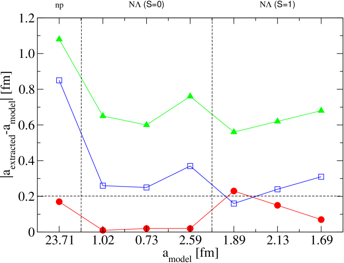
Figure 1: (Color online) Comparison of different extraction methods for the scattering length $a$. Shown are the differences between results predicted by various $YN$ and $NN$ models and corresponding values extracted via the dispersion integral method (circles), the Jost-ERA approach (9) (squares) and the Migdal-Watson prescription (10) (triangles). The lines are drawn to guide the eye.

The systematic offset inherent in the Jost-ERA approach as well as in the Migdal-Watson prescription can be best seen in Fig. 1, where we shown the difference between the scattering lengths predicted by various models and the values extracted via the dispersion integral (circles), the Jost-ERA method (squares) and the Migdal-Watson prescription (triangles).

While the Jost-ERA approach might still be a reasonable tool for getting a first rough estimate of the scattering length for a particular two-body interaction one should be rather cautious when using it for more quantitative analyses. In particular, its application in a combined fit to elastic scattering data and invariant mass spectra, e.g. to $\Lambda p$ and $pp\to K^{+}\Lambda p$, is rather problematic and can easily cause misleading results. Because of the offset in the scattering length in applications to final-state effects it is clear that a combined fit cannot converge to a unique (the “true”) $\Lambda p$ scattering length. Only the elastic data will favour values close to the “true” scattering length whereas the production data tend to support larger (negative) values. This is obvious from the corresponding Jost-ERA results presented in Table 1 and also from Fig. 1. We believe that the analysis of Hinterberger and Sibirtsev presented in Ref. Hinter is an instructive exemplification of this dilemma. Employing the Jost-ERA approach to low energy total $\Lambda p$ cross sections Alex ; Sechi and to experimental results for the missing mass spectrum of the reaction $pp\to K^{+}X$ Siebert separately, they derived (spin averaged) scattering lengths of $a=-1.81^{+0.18}_{-0.21}$ fm and $a=-2.57^{+0.20}_{-0.23}$ fm, respectively. Taking into account the error bars this is roughly the difference we would expect from the offset (of around $0.3$ fm) seen in our test calculations and, therefore, one must consider the results as being practically consistent with each other. But the authors of Ref. Hinter attempted to “reconcile” the results even more by introducing a spin-dependence in the fitting procedure. Indeed, with the relative magnitude of singlet to triplet contribution in the production reaction as free parameter (their relative strength in the elastic channel is fixed at 1:3 by the spin weight!) a “fully consistent” description of the combined data could be achieved Hinter and apparently the spin-singlet as well as spin-triplet $\Lambda p$ $S$-wave scattering lengths could be determined from spin-averaged observables. Our experience with the Jost-ERA approach reported above, however, strongly suggests that the sensitivity to the spin seen in this analysis is most likely just an artifact of the method applied.

Table 2: $S$-wave effective ranges $r_{e}$ (in fm) for various $YN$ NijV ; Melni2 and $NN$ Argonne potentials. The results for the original models are compared with those obtained by applying the dispersion integral method (7) and the approximation Eq. (9) (Jost-ERA).

model	exact result	disp.int.	Jost-ERA
Jülich 01 singlet	4.49	4.31	2.48
Nijmegen 97a singlet	6.01	4.78	2.81
Nijmegen 97f singlet	3.05	2.82	1.60
Jülich 01 triplet	2.57	2.49	1.89
Nijmegen 97a triplet	2.74	2.60	1.70
Nijmegen 97f triplet	3.34	2.67	1.69
Argonne v14 singlet	2.78	2.91	0.43

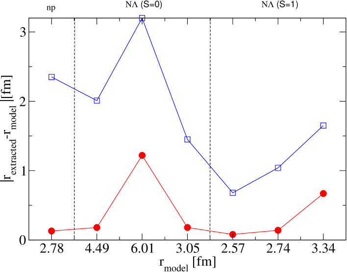
Figure 2: (Color online) Comparison of different extraction methods for the effective range $r_{e}$. Shown are the differences between results predicted by various $YN$ and $NN$ models and corresponding values extracted via the dispersion integral method (circles) and the Jost-ERA approach (9) (squares). The lines are drawn to guide the eye.

Let us now come to the effective range $r_{e}$. Since the dispersion relations yield only an integral representation for the product $a^{2}((2/3)a-r_{e})$ but not for the effective range $r_{e}$ alone Gasparyan2003 it follows that the attainable accuracy of $r_{e}$ is always limited roughly by twice the relative error on $a$. Still, it is interesting to see what values one gets for $r_{e}$ from the dispersion integrals. Corresponding results are presented in Table 2 and in Fig. 2. Evidently, the values extracted via the dispersion integral agree much better with the original results as one might have expected. In fact, in practically all cases the deviation is in the order of only 5 % or even less. This suggests that one could use the dispersion integrals also to extract the effective range $r_{e}$ from data. But one should keep in mind that, unlike the case of the scattering length, now one cannot rely on a solid and general estimate of the uncertainty. As far as the Jost-ERA approach is concerned it is clear from Table 2 that it yields rather poor results. In case of the Migdal-Watson prescription (10) it turned out that the fit always prefers an effective range $r_{e}$ equal to zero. This is due to the term proportional to $r^{2}_{e}p^{4}$ in the denominator of the $A(m^{2})$ that make the production cross section decrease too fast as compared to the data (or to our calculations with realistic models). Therefore we don’t show any results of the Migdal-Watson fit for $r_{e}$.

One should note here that the upper limit in the dispersion integrals was always taken such that $p_{max}=205$ MeV/c (as in Gasparyan2003 ) that corresponds to $\epsilon_{max}\equiv m_{max}-m_{0}\approx 40$ MeV for the $\Lambda N$ and $\Sigma N$ systems and $\epsilon_{max}\approx 45$ MeV for the $NN$ system. In the latter case it is interesting to see what happens if one varies the range of integration, since the energy structure in the $NN$ interaction is much narrower due to the large $NN$ scattering length. For $\epsilon_{max}=10$ MeV and $\epsilon_{max}=20$ MeV as upper limits of the integration one gets the scattering lengths $a=-22.62$ fm and $a=-23.17$ fm, respectively – which are in principle still close to the original value. For the effective range, however, the calculation yields $r_{e}=4.78$ fm and $3.72$ fm, respectively. The reason why the agreement for $\epsilon_{max}>40$ MeV is so good is that the $NN$ ${}^{1}S_{0}$ phase shift becomes sufficiently small at such energies, which implies a small uncertainty according to the error estimation in Ref. Gasparyan2003 .

IV Dispersion relation in the presence of Coulomb repulsion

In the case when both baryons in the final state carry charges (for example in the reaction $pp\to K^{0}p\Sigma^{+}$) there is a Coulomb interaction between them. Then the production amplitude $A(m^{2})$ acquires additional singularities at $p=0$, due to the long-range nature of the Coulomb forces, and the formalism developed in Sect. 2 is no longer applicable directly. In this section we want to describe the modifications that are necessary in order to adapt the dispersion-relation method to the situation when the Coulomb force is present in the final-state interaction. We restrict ourselves to the case of a repulsive Coulomb interaction so that no bound states are present.

In order to elucidate the principle idea we start out from the case of elastic (two-body) scattering. Here the problem can be most conveniently dealt with by applying the Gell-Mann–Goldberger two-potential formalism Gell . Let us assume that the total potential $V=V_{c}+V_{s}$ is given by the sum of a short-ranged hadronic potential $V_{s}$ and the Coulomb interaction $V_{c}$. Then the total reaction amplitude $T$ can be written as $T=T_{c}+T_{cs}$, where $T_{c}$ is the Coulomb amplitude and $T_{cs}$ is defined by

$$T_{cs}=(1+T_{c}G_{0})t_{cs}(1+G_{0}T_{c}),$$ (11)

where $t_{cs}$ fulfils a Lippmann-Schwinger equation,

$$t_{cs}=V_{s}+V_{s}G_{c}t_{cs},$$ (12)

with the short-range potential $V_{s}$ as driving term. To obtain the physical on-shell amplitudes one needs to project the corresponding $T$-operators on the so-called Coulombian asymptotic states $\textstyle{\>\left|\>\!p_{\infty}\pm\>\!\right\rangle}$ which are related to the Coulomb scattering states (with fixed angular momentum – in our case $l=0$) $\textstyle{\>\left|\>\!p\pm\>\!\right\rangle}_{c}$ via $\textstyle{\>\left|\>\!p\pm\>\!\right\rangle}_{c}=\textstyle{\>\left|\>\!p_{\infty}\pm\>\!\right\rangle}+G_{0}^{\pm}T_{c}^{\pm}\textstyle{\>\left|\>\!p_{\infty}\pm\>\!\right\rangle}$ vanHaeringen1976 . Here $p$ denotes the center of mass momentum in the baryon-baryon system. In this way one obtains in particular

$${}_{c}\textstyle{\left\langle\,p-\,\right|\>}t_{cs}\textstyle{\>\left|\>\!p+\>\!\right\rangle}_{c}=-\frac{1}{\pi\mu}f_{cs}(p),$$ (13)

where $f_{cs}$ is the so-called Coulomb-modified nuclear scattering amplitude and $\mu$ is the reduced mass. Its relation to the phase shift $\delta_{cs}$ is the following

$$f_{cs}=\frac{e^{2i\delta_{c}}(e^{2i\delta_{cs}}-1)}{2ip},$$ (14)

with $\delta_{c}$ denoting the pure Coulomb $S$-wave phase shift given by $\delta_{c}=\arg{(\Gamma(1+i\eta))}$ with $\eta=\frac{\mu e^{2}}{p}$.

It has been shown in Ref. Hamilton1973 under rather general assumptions that the modified amplitude $\tilde{f}(p)=e^{-2i\delta_{c}}f_{cs}(p)/C^{2}(p)$ is free of the Coulomb singularities on the physical sheet and possesses only the singularities caused by dynamical cuts (see also Refs. Cornille1962 ; vanHaeringen1977 ; Heller1966 ; Scotti1965 ). In addition below the inelastic cuts and above the two-baryon threshold the modified unitarity relation reads

$$\tilde{f}(s+i0)-\tilde{f}(s-i0)=2ip\tilde{f}(p)\tilde{f}^{*}(p)C^{2}(p)$$ (15)

with $C^{2}(p)=\frac{2\pi\eta}{e^{2\pi\eta}-1}$ being the Coulomb penetration factor.

Furthermore an effective range function, modified for the presence of the Coulomb interaction, can be defined as well. Is is given by

$$S(p)\equiv pC^{2}(p)\cot\delta_{cs}(p)+Q(p)=-1/a_{cs}+r_{e}p^{2}/2+..,$$ (16)

where $Q(p)\equiv\mu e^{2}[\psi(i\eta)+\psi(-i\eta)-2\ln\eta],\ \psi(z)=\Gamma^{\prime}(z)/\Gamma(z)$.

Coming back now to the production reaction it can be analogously shown that also the modified production amplitude

$$\tilde{A}(m^{2})=e^{-i\delta_{c}}A(m^{2})/C(p)$$ (17)

is free of the aforementioned singularities Hamilton1973 . Therefore a dispersion relation similar to Eq. (1) can be written down

$$\tilde{A}(m^{2})=\frac{1}{\pi}\int_{-\infty}^{\tilde{m}\,^{2}}\frac{\tilde{D}(m^{\prime}\,{}^{2})}{m^{\prime}\,{}^{2}-m^{2}}dm^{\prime}\,{}^{2}+\frac{1}{\pi}\int_{m_{0}^{2}}^{\infty}\frac{\tilde{D}(m^{\prime}\,{}^{2})}{m^{\prime}\,{}^{2}-m^{2}}dm^{\prime}\,{}^{2}.$$ (18)

Unitarity implies that the discontinuity for the elastic cut is

$$\tilde{D}(m^{2})=\tilde{A}(m^{2})e^{-i\delta_{cs}}\sin{\delta_{cs}}.$$ (19)

The solution to Eq. (18) is found in complete analogy to the case without the presence of the Coulomb interaction,

$$\tilde{A}(m^{2})=\exp\left[{\frac{1}{\pi}\int_{m_{0}^{2}}^{m_{max}^{2}}\frac{\delta_{cs}(m^{\prime}\,{}^{2})}{m^{\prime}\,{}^{2}-m^{2}-i0}dm^{\prime}\,{}^{2}}\right]\tilde{\Psi}(m^{2})\ ,$$ (20)

where $\tilde{\Psi}(m^{2})$ is some function slowly varying with $m^{2}$. If one neglects the the weak $m^{2}$ dependence present in $\tilde{\Psi}(m^{2})$ the expression for the phase shift $\delta_{cs}$ in terms of the differential cross section becomes

$$\frac{\delta_{cs}(m^{2})}{\sqrt{m^{2}-m_{0}^{2}}}=-\frac{1}{2\pi}{\bf P}\int_{m_{0}^{2}}^{m_{max}^{2}}\frac{\log{\left[\displaystyle{\frac{1}{p^{\prime}C^{2}(p^{\prime})}\frac{d^{2}\sigma}{dm^{\prime}\,{}^{2}dt}}\right]}}{\sqrt{m^{\prime}\,{}^{2}-m_{0}^{2}}\ (m^{\prime}\,{}^{2}-m^{2})}\sqrt{\frac{m_{max}^{2}-m^{2}}{m_{max}^{2}-m^{\prime}\,{}^{2}}}dm^{\prime}\,{}^{2}.$$ (21)

Using the effective range expansion (16) one can then extract the scattering length $a_{cs}$ from this dispersion integral.

V Test of the method for the Coulomb case

One of the obvious reactions for applying the formalism with Coulomb is $pp\to K^{0}\Sigma^{+}p$ where one could determine the $\Sigma N$ scattering length for the isospin 3/2 state. Note that the $\Sigma^{+}p$ channel does not couple to the $\Lambda N$ system and is therefore free of inelastic cuts (that start already on the left-hand side) as required for the applicability of the disperson integral method. For this reaction one could perform a model calculation analogous to the one for $pp\to K^{+}\Lambda p$ model which we used for testing the dispersion-integral method in the absence of the Coulomb interaction Gasparyan2003 . However, the implementation of Coulomb effects into our momentum-space code is technically complicated and requires also some approximations Hanhart . Thus, for the present test calculation we adopt a different strategy. First, instead of the momentum-space $YN$ models of Refs. Holz ; Melni2 ; Haiden we take the r-space Argonne ($NN$) potential, however, with parameters modified in such a way that the effective range parameters are similar to those predicted by realistic $YN$ potentials Holz ; NijV ; Melni2 ; Haiden for the $\Sigma N$ $I=3/2$ ${}^{1}S_{0}$ partial wave. In particular we prepared two models with Coulomb modified scattering length of $a_{cs}=-3.24$ fm (model 1) and $a_{cs}=-1.86$ fm (model 2), respectively. The corresponding scattering lengths without Coulomb interaction are $-4.11$ fm and $-2.01$ fm, respectively. For the transition amplitude we use the scattering wave function calculated from those potential models and evaluated at the origin. This corresponds to the assumption that the production operator is point-like, which is reasonable as long as we are interested only in the mass dependence of the production amplitude. The corrections stemming from a possible mass dependence of the production operator were discussed in Ref. Gasparyan2003 .

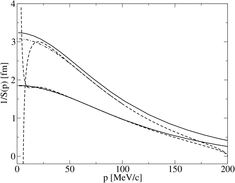
Figure 3: The inverse of the effective range function $S(p)$ for model 1 (upper curves) and model 2 (lower curves). The solid lines denote the phase shifts predicted by the corresponding model, whereas the dashed lines correspond to the phase shift extracted via Eq. (21). The dash-dotted lines show the result of the smooth extrapolation of the dashed lines, as explained in the text.

The results of applying Eq. (7) with $m_{max}-m_{0}=40$ MeV ($p_{max}=205$ MeV/c) are shown in Fig. 3, where we plot the function $1/S(p)$ which should coincide with the scattering length $-a_{cs}$ at $p=0$. Obviously, there is a strongly nonanalytic behavior of the extracted inverse effective range function when approaching the threshold – which, however, can be easily understood. It is clear from Eq. (16) that the threshold behavior of the Coulomb modified phase shift is $\delta_{cs}\approx-a_{cs}\,p\,C^{2}(p)$, i.e. $\delta_{cs}$ goes to zero very rapidly. To obtain such a behavior on the left-hand side of Eq. (21) one needs to have a very precise cancellation in the integral on the right-hand side of Eq. (21) that is, of course, impossible if one truncates the integral at a finite momentum. But still one can expect for Eq. (21) to work for momenta not too close to the threshold, namely above the typical Coulomb scale of $2\pi\alpha/\mu\approx 25$ MeV/c where the factors $C^{2}(p)$ and $Q(p)$ that appear in the effective range function (Eq. (16)) become smoother. This is indeed the case, as can be seen from Fig. 3. Thus, a natural and practical step here would be to extrapolate the extracted $S(p)$ to the threshold from above. Using a 4-th order polynomial of the type $-1/a_{cs}+r_{e}p^{2}/2-Pr_{e}^{3}p^{4}$ and fixing the coefficients in the region $50-100$ MeV/c, i.e. well above the Coulomb structure, one can then extrapolate $S(p)$ to the threshold, cf. the dash-dotted lines in Fig. 3. In this case one gets a satisfactory agreement between the true and extracted scattering lengths. In fact, the deviations are not worse then in the case when we consider the same potentials without Coulomb interaction and they are also within the theoretical error of 0.3 fm estimated in Ref. Gasparyan2003 . The extracted values are $a_{cs}=-3.10$ fm and $a_{cs}=-1.86$ fm for models 1 and 2, respectively, with Coulomb, and $a_{s}=-4.05$ fm and $a_{s}=-2.06$ fm when the Coulomb interaction is switched off. We also checked that the sensitivity of the result to the region of interpolation of the effecitve range function $S(p)$ is rather low. For instance if one shifts the lower bound of this region to $70$ MeV/c the corresponding change in the scattering length will be less then $0.05$ fm.

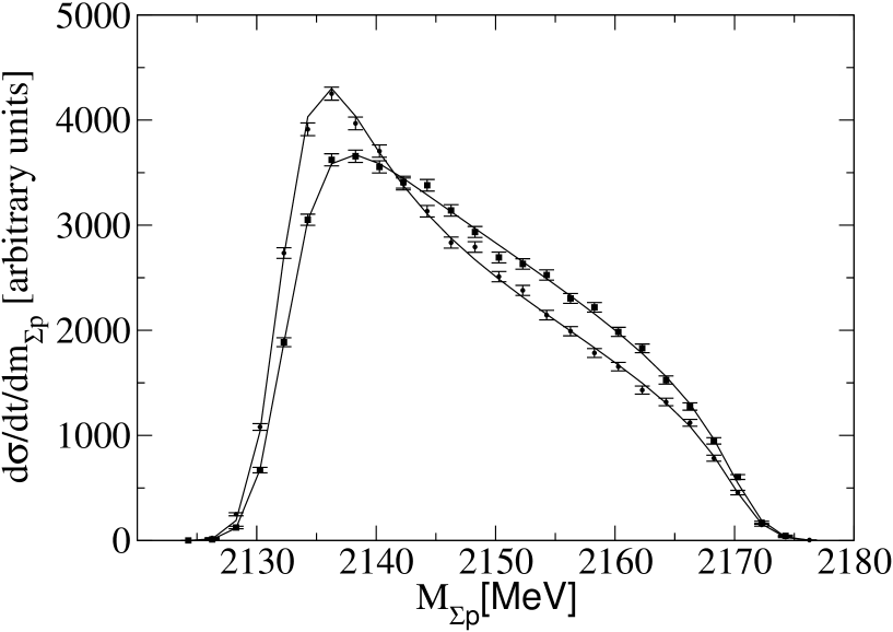
Figure 4: Pseudo data for the differential $\Sigma^{+}p$ cross section generated from model 1 (circles) and model 2 (squares) as a function of the $\Sigma p$ invariant mass $M_{\Sigma p}$ with corresponding fit by the exponential parameterization Eq. (22).

If one wishes to consider a more realistic situation, one needs to deal with mass distributions with finite statistical errors, finite mass resolution, and finite binning. To examine also this situation we have generated two data sets, corresponding to the models 1 and 2 as shown on Fig. 4. We have chosen the binning as well as the mass resolution to be equal to $2$ MeV (the same as in the experiment Siebert that was analyzed in Gasparyan2003 ), and the statistics to be rather high in order to minimize the influence of the statistical error bars on the results. The excess energy was set to $40$ MeV to simplify the simulation. In a realistic situation larger values are preferable to minimize the influence of the meson-baryon interactions, cf. the corresponding remarks in Ref. Gasparyan2003 . In our test calculation such meson-baryon interactions are neglected anyway.

We start here with the procedure suggested in appendix A of Gasparyan2003 , namely by fitting the cross section with an exponential parameterization of the type

$$\frac{d^{2}\sigma}{dm\,^{2}dt}=C^{2}(p)\times\exp{\left[C_{0}+\frac{C_{1}^{2}}{(m^{2}-C_{2}^{2})}\right]}\times\text{phase space}\ .$$ (22)

This formula fits the generated cross section with the $\chi^{2}$ per degree of freedom of $\chi^{2}_{dof}\sim 1$, cf. Fig. 4. A new problem that arises here is that the production amplitude contains a very narrow structure (of the size $2\pi\alpha/\mu$) close to threshold as can be seen in Fig. 5 (solid lines). Clearly, this structure can not be reproduced after the fitting procedure as it gets smeared out by the mass resolution and binning (their size is much larger than the scale of the structure). The amplitudes coming from the fit are depicted in Fig. 5 by dash-dotted lines. However the fit can be improved if one notes that the structure comes mostly from the part of the dispersion integral (20) containing the leading term in the $\delta_{cs}$ expansion near the threshold, namely (in the nonrelativistic case)

$$\exp\left[{\frac{1}{\pi}\int_{0}^{\infty}\frac{-a_{cs}C^{2}(p^{\prime})}{p^{\prime}\,{}^{2}-p^{2}-i0}\left(\frac{p^{2}}{p^{\prime 2}}\right)dp^{\prime}\,{}^{2}}\right]=\exp\left[-a_{cs}Q(p)\right],$$ (23)

where we made a subtraction at $p=0$ to render the integral convergent. This does not change the energy dependence of the resulting exponent. Indeed the structure disappears after dividing the production amplitude by the factor $\exp[-a_{cs}Q(p)]$.

Obviously the scattering length is unknown before its extraction! But what can be done is to resort to an iterative procedure including first the extraction of the unimproved scattering length, then putting it into the fit function,

$$\frac{d^{2}\sigma}{dm\,^{2}dt}=C^{2}(p)\times\exp{\left[C_{0}+\frac{C_{1}^{2}}{(m^{2}-C_{2}^{2})}-2a_{cs}Q(p)\right]}\times\text{phase space}\ ,$$ (24)

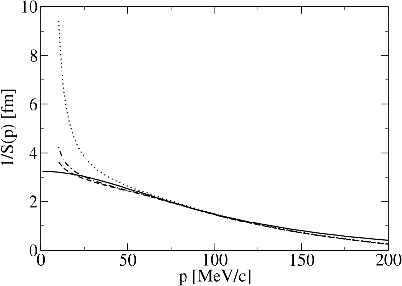
Figure 6: The inverse of the effective range function $S(p)$ calculated by means of the iterative procedure as discussed in the text. The dotted line corresponds to the zeroth iteration, the dashed line corresponds to the first iteration, and the dash-dotted line corresponds to the second iteration. The solid curve denotes the exact result. Shown are results for the model 1.

and repeating this step until the procedure converges. Fortunately the iterations converge already after three or four iterations, and the resulting amplitudes are shown in Fig. 5 by the dashed lines. The improvement of the fit is quite obvious. Finally we applied the combination of the extrapolation and iteration procedures to obtain the scattering lengths from the pseudodata. Since the data have a statistical uncertainty we generated a sample of 1000 mass distributions and looked at the average value of the scattering lengths. They turned out to be $-2.89\pm 0.06$ fm for model 1 and $-1.82\pm 0.05$ for model 2. Note that the deviation from the correct values is now a bit larger, but still reasonable ($~{}0.35$ fm in the worst case). Fig. 6 shows how the extracted inverse effective range function approaches to the correct one given by the model by the example of model 1.

VI Summary

In a recent publication Gasparyan2003 we have presented a formalism based on dispersion relations that allows one to relate spectra from large-momentum transfer reactions, such as $pp\to K^{+}p\Lambda$ or $\gamma d\to K^{+}n\Lambda$, directly to the scattering length of the interaction of the final-state particles. An estimation of the systematic uncertainties of that method, relying on general arguments, led to the conclusion that the theoretical error in the extracted scattering length should be less than 0.3 fm. This finding was corroborated in an application of the method to results of a microscopic model calculation for $pp\to K^{+}p\Lambda$.

In the present paper this dispersion theoretical method was generalized to the case where a repulsive Coulomb force is present in the final-state interaction. As an example let us mention the reaction $pp\to K^{0}p\Sigma^{+}$ which could be used to extract the $p\Sigma^{+}$ scattering length. Though the generalization of the formalism itself is straight forward it turned out that there are some additional features due to the Coulomb interaction which need to be taken into account in concrete applications of the method to data. These practical aspects were thoroughly discussed and it was shown how to circumvent the difficulties. In a test calculation utilizing potential models with effective range parameters similar to those of realistic $YN$ interactions the extracted values for the scattering lengths were found to agree within 0.3 fm with those predicted by the models. Thus, the accuracy of the dispersion theoretical method for extracting the scattering lengths from final-state interactions with Coulomb force is comparable to the case where no Coulomb interaction is present.

We presented also a more detailed examination of the accuracy of the dispersion-integral method than in Ref. Gasparyan2003 . In particular we considered final-state interactions of varying strengths, corresponding to a much larger range of values of the scattering length. These investigations confirmed the reliability of the general error estimate provided in Ref. Gasparyan2003 . Indeed in most of the considered cases the deviation of the extracted scattering length from the true value was significantly smaller than the uncertainty of 0.3 fm derived in that paper. In addition we studied the effective range $r_{e}$ which can be also extracted by the proposed dispersion-integral method. For most of the interaction models considered the extracted values of $r_{e}$ agreed remarkably good with the true results. Thus, it might be sensible to use the proposed method to extract the effective range from data - though one should always keep in mind that for this quantity a generally valid error estimation is not possible Gasparyan2003 .

Finally, we compared the present method with the performance of other, approximative treatments of the final-state interaction that are commonly used in the literature to extract information on the scattering length and also the effective range. In particular we tested the Jost-function approach based on the effective-range approximation (Jost-ERA) and an even simpler approach that relies simply on utilizing the effective range approximation itself. Thereby, we showed that the latter methods lead to systematic deviations from the true values of the scattering lengths in the order of 0.3 fm (Jost-ERA) and even 0.7 fm (direct effective-range approximation). This suggests that one should be rather cautious in the interpretation of results achieved with those methods.

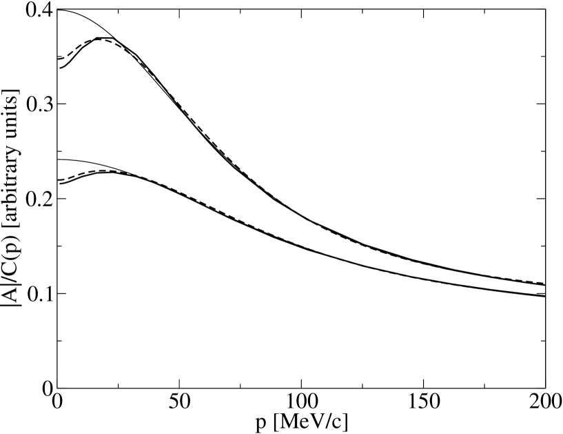
Figure 5: The production amplitude $A(m^{2})$ divided by the factor $C(p)$ for model 1 (upper curves) and model 2 (lower curves). The solid lines are the amplitudes as calculated from the models. The dash-dotted lines correspond to the fitted amplitudes. The dashed lines denote the fitted amplitudes improved by the iterative procedure as discussed in the text.

- (1) See, e.g., C.J. Joachain, Quantum Collision Theory, (North-Holland, Amsterdam 1975).
- (2) G.A. Miller, B.M.K. Nefkens, and I. Slaus, Phys. Rep. 194, 1 (1990).
- (3) C.B. Dover and H. Feshbach, Ann. Phys. 198, 321 (1990).
- (4) J. Gasser, H. Leutwyler and M. E. Sainio, Phys. Lett. B 253, 252 (1991).
- (5) S. Wycech, A.M. Green, and J.A. Niskanen, Phys. Rev. C 52, 544 (1995).
- (6) S.A. Rakityansky, S.A. Sofianos, W. Sandhas, and V.B. Belyaev, Phys. Lett. B 359, 33 (1995).
- (7) V.B. Belyaev, S.A. Rakityansky, S.A. Sofianos, M. Braun, and W. Sandhas, Few. Body. Syst. Suppl. 8, 309 (1995).
- (8) S.A. Rakityansky, S.A. Sofianos, M. Braun, V.B. Belyaev and W. Sandhas, Phys. Rev. C 53, R2043 (1996).
- (9) A. Fix and H. Arenhövel, Phys. Rev. C 66, 024002 (2002).
- (10) A. Sibirtsev, J. Haidenbauer, J.A. Niskanen, and Ulf-G. Meißner, Phys. Rev. C 70, 047001 (2004).
- (11) J.A. Niskanen, A. Sibirtsev, J. Haidenbauer, and C. Hanhart, Int. J. Mod. Phys. A 20, 634 (2005).
- (12) Q. Haider and L.C. Liu, Phys. Rev. C 66, 045208 (2002).
- (13) V. Antonelli, A. Gall, J. Gasser and A. Rusetsky, Ann. Phys. 286, 108 (2001).
- (14) D. Gotta, Prog. Part. Nucl. Phys. 52, 133 (2004).
- (15) W.R. Gibbs, S.A. Coon, H.K. Han, and B.F. Gibson, Phys. Rev. C 61, 064003 (2000).
- (16) D.E. González Trotter et al., Phys. Rev. Lett. 83, 3788 (1999).
- (17) V. Huhn et al., Phys. Rev. C 63, 014003 (2000).
- (18) J. Deng, A. Siepe, and W. von Witsch, Phys. Rev. C 66, 047001 (2002).
- (19) S. R. Beane, V. Bernard, E. Epelbaum, U. G. Meissner and D. R. Phillips, Nucl. Phys. A 720 (2003) 399 [arXiv:hep-ph/0206219]; A. Gardestig and D. R. Phillips, arXiv:nucl-th/0501049;
- (20) V. Lensky, V. Baru, J. Haidenbauer, C. Hanhart, A. E. Kudryavtsev and U. G. Meissner, arXiv:nucl-th/0505039.
- (21) A. Gasparyan, J. Haidenbauer, C. Hanhart and J. Speth, Phys. Rev. C 69, 034006 (2004)
- (22) J. T. Balewski et al., Phys. Lett. B 420, 211 (1998); S. Sewerin et al., Phys. Rev. Lett. 83, 682 (1999).
- (23) R. Bilger et al., Phys. Lett. B 420, 217 (1998).
- (24) J. T. Balewski et al., Eur. Phys. J. A 2, 99 (1998).
- (25) F.M. Renard and Y. Renard, Nucl. Phys. B1, 389 (1967).
- (26) B.O. Kerbikov, B.L.G. Bakker, and R. Daling, Nucl. Phys. A480, 585 (1988); B.O. Kerbikov, Phys. Atom. Nucl. 64, 1835 (2001).
- (27) B. Mecking et al., CEBAF proposal PR-89-045 (1989).
- (28) R.A. Adelseck and L.E. Wright, Phys. Rev. C 39, 580 (1989).
- (29) X. Li and L.E. Wright, J. Phys. G 17, 1127 (1991).
- (30) H. Yamamura, K. Miyagawa, T. Mart, C. Bennhold, H. Haberzettl, and W. Glöckle, Phys. Rev. C 61, 014001 (1999).
- (31) C.R. Howell et al., Phys. Lett. B 444, 252 (1998).
- (32) see, e.g., F. A. Harris, Int. J. Mod. Phys. A20, 445 (2005), and references therein.
- (33) see, e.g., J. Schumann, hep-ex/0505098, and references therein.
- (34) M. Goldberger and K.M. Watson, Collision Theory (Wiley, New York, 1964).
- (35) K. Watson, Phys. Rev. 88, 1163 (1952); A.B. Migdal, Sov. Phys. JETP 1, 2 (1955).
- (36) B. V. Geshkenbein, Yad. Fiz. 9, 1232 (1969) [Sov. J. Nucl. Phys. 9, 720 (1969)].
- (37) B. V. Geshkenbein, Phys. Rev. D 61, 033009 (2000).
- (38) N. I. Muskhelishvili, Singular Integral Equations, (P. Noordhof N. V., Groningen, 1953).
- (39) R. Omnes, Nuovo Cim. 8, 316 (1958).
- (40) W. R. Frazer and J. R. Fulco, Phys. Rev. Lett. 2, 365 (1959).
- (41) J. T. Balewski et al., Phys. Lett. B 420, 211 (1998); S. Sewerin et al., Phys. Rev. Lett. 83, 682 (1999).
- (42) F. Hinterberger and A. Sibirtsev, Eur. Phys. J. A 21, 313 (2004).
- (43) B. Holzenkamp, K. Holinde, and J. Speth, Nucl. Phys. A500, 485 (1989).
- (44) Th.A. Rijken, V.G. Stoks, and Y. Yamamoto, Phys. Rev. C 59, 21 (1999).
- (45) J. Haidenbauer, W. Melnitchouk and J. Speth, AIP Conf. Proc. 603, 421 (2001), [arXiv:nucl-th/0108062].
- (46) J. Haidenbauer and U.-G. Meißner, nucl-th/0506019.
- (47) A. Gasparian, J. Haidenbauer, C. Hanhart, L. Kondratyuk and J. Speth, Phys. Lett. B 480, 273 (2000).
- (48) R.B. Wiringa, R.A. Smith, and T.L. Ainsworth, Phys. Rev. C 29, 1207 (1984).
- (49) G. Alexander et al., Phys. Rev. 173, 1452 (1968).
- (50) B. Sechi-Zorn et al., Phys. Rev. 175, 1735 (1968).
- (51) R. Siebert et al., Nucl. Phys. A 567, 819 (1994).
- (52) M. Gell-Mann and M.L. Goldberger, Phys. Rev. 91, 398 (1953).
- (53) H. van Haeringen, J. Math. Phys. 17, 995 (1976).
- (54) J. Hamilton, I. Oeverboe and B. Tromborg, Nucl. Phys. B 60, 443 (1973).
- (55) H. Cornille and A. Martine, Nuovo Cimento 26, 298 (1962).
- (56) H. van Haeringen, J. Math. Phys. 18, 927 (1977).
- (57) L. Heller and M. Rich, Phys. Rev. 144, 1324 (1966)
- (58) A. Scotti and D. Y. Wong, Phys. Rev. 138, B145 (1965)
- (59) C. Hanhart, J. Haidenbauer, A. Reuber, C. Schütz, and J. Speth, Phys. Lett. B 358, 21 (1995).