Relativistic Model of Triquark Structure

Abstract

At this point it is still unclear whether pentaquarks exist. While they have be seen in some experiments there are many experiments in which they are not found. On the assumption that pentaquarks exist, several authors have studied the properties of pentaquarks. One description considered is that of pentaquarks which consist of a diquark coupled to a triquark. There is a quite extensive literature concerning the properties of diquarks and their importance in the description of the nucleon has been considered by several authors. On the other hand, there is little work reported concerning the description of triquarks. In the present work we study a model for the triquark in which it is composed of a component which contains a quark coupled to a scalar diquark and another two components in which there is a quark coupled to a kaon. We solve for the wave function of the triquark and obtain a mass for the triquark of 0.81 GeV which is quite close to the value of 0.80 GeV obtained in a QCD sum rule study of triquark properties.

I INTRODUCTION

There has been a great deal of interest in the study of pentaquarks and a large number of experiments have been carried out [1-11]. The existence of pentaquarks is uncertain since they have been seen in some experiments and not in others. Various groups hope to clarify this situation by performing more precise experimental searches. The $\Theta^{+}(1540)$ which decays to a kaon and a nucleon has been seen in several experiments. It has been interpreted as a pentaquark with a $udud\bar{s}$ structure [12]. A pentaquark $\Theta_{c}^{0}$ with the assumed structure $udud\bar{c}$ has also been observed recently. A recent review may be found in Ref. [13].

We were particularly interested in the diquark-triquark model of Karliner and Lipkin which has been applied in the study of pentaquarks [14,15], and we have made use of a variant of that model in our work [16,17]. One problem for the theorist has been the very small widths of the observed pentaquarks. We have studied that question in a relativistic diquark-triquark model and found we could explain the small widths seen in experiment [16,17]. In our model, as in that of Refs. [14,15], the pentaquark is described as scalar diquark coupled to a triquark. [See Fig. 1.] Using the insight gained in our analysis of the nucleon, which made use of a quark-diquark model [18], we took the scalar diquark mass to be 400 MeV in our study of the pentaquark.

There have been many studies of diquark structure making use of the Nambu-Jona-Lasinio (NJL) model. Some of that work is reviewed in Ref. [19]. One may suggest that, in addition to studies of diquark structure, a study of triquark structure may be of interest. In our earlier work the triquark mass was taken to be 800 MeV on phenomenological grounds. We note that a calculation of triquark properties, using the operator product expansion and including direct instanton contributions, obtained a triquark of $ud\bar{s}$ structure of mass 800 MeV [20]. An additional triquark state was found at 900 MeV in Ref. [20]. (Another work making use of QCD sum rules yields quite small values for the width of the $\Theta^{+}(1540)$ pentaquark [21].)

Once we decide to study triquark structure, we face the following problem. The triquark of mass 800 MeV is very close to the threshold for decay to a 400 MeV diquark and a 450 MeV strange quark. Similarly, the triquark mass is close to the mass of a $u$ (or $d$) quark of 350 MeV and a kaon of mass 495 MeV. This difficultly cannot be overcome by including a confinement model since there is no confining interaction between a kaon and a quark. Therefore, in the present work we have made use of the quark propagator obtained in Ref. [22]. In that work we considered quark propagation in the presence of a gluon condensate and found that the quark propagator had no on-mass-shell poles. That is, the quark was a non-propagating mode in the presence of the condensate. As we will see, the use of the quark propagator of Ref. [22] enables us to proceed in our analysis of triquark structure. (In an early work we used the form of the propagator discussed in Ref. [22] in a study of nontopological solitons [23].)

The organization of our work is as follows. In Section II we review our model of quark propagation in the presence of a gluon condensate. In that model the quark propagator has no on-mass-shell poles. In Section III we present the equation for the vertex describing triquark decay to the channels: i) a $u$ quark plus a $\emph{K}^{0}$ meson, ii) a scalar diquark plus a $\bar{s}$ quark and iii) a $d$ quark and a $\emph{K}^{+}$ meson. [See Figs. 2-4.] In Section IV we describe the results of our analysis and in Section V we present some further comments and conclusions. The Appendix contains a discussion of the normalization of the wave functions of the scalar diquark and the kaon.

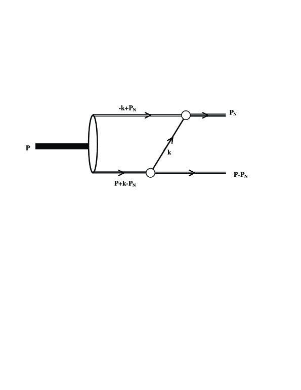
Figure 1: In this figure the heavy line denotes the pentaquark and the line of momentum $-k+P_{N}$ denotes an on-mass-shell diquark. The line of momentum $k$ represents the quark and $P+k-P_{N}$ is the momentum of the triquark. In the final state we have a baryon of momentum $P_{N}$ and a meson of momentum $P-P_{N}$.

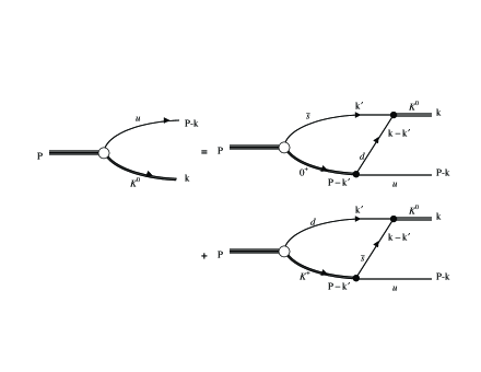
Figure 2: The equation for the triquark vertex function for the $K^{0}$ and $u$ quark component.

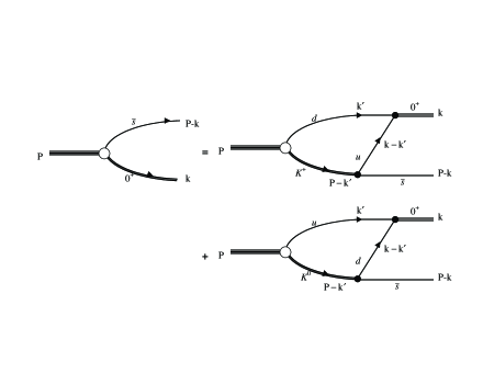
Figure 3: The equation for the triquark vertex function for the diquark and $\bar{s}$ quark component.

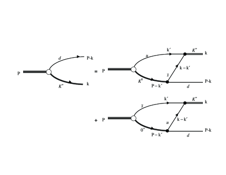
Figure 4: The equation for the triquark vertex function for the $K^{+}$ and $d$ quark component.

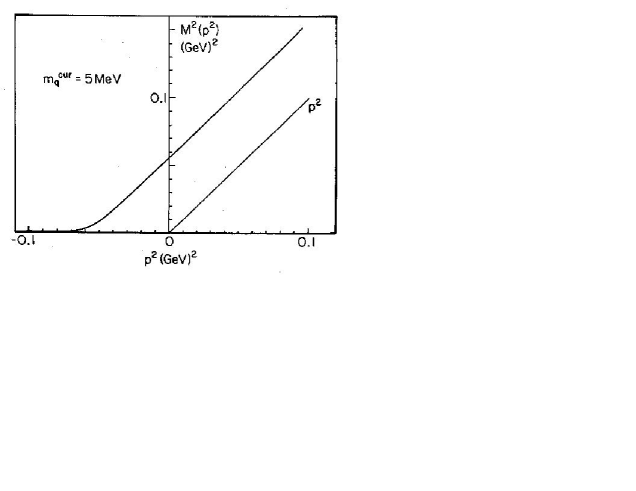
Figure 5: The square of the dynamical mass, $M^{2}(p^{2})$, for up and down quarks. Here we chose $m_{q}^{cur}=5$ MeV. [For $p^{2}>0,M^{2}(p^{2})=p^{2}+\kappa^{2}$.]

II Quark Propagator in The Presence of a Gluon Condensate

In an earlier work we discussed quark propagator in the presence of a condensate of the form $<g^{2}A^{a}_{\mu}A^{\mu}_{a}>$ which has recently been shown to be the Landau gauge version of a more general gauge invariant expression. We have discussed quark propagation in the presence of such a condensate treating the vacuum as a random medium of gluon fields [22]. It is found that the quark propagator has no on-mass-shell poles indicating that the quark cannot propagate over extended distances. As an example, we show one of the momentum-dependent mass functions obtained in our model in Fig. 5. It may be seen that the equation $p^{2}-M^{2}(p^{2})=0$ has no solution. In our work we have modified the solution shown in Fig. 5 to have a constituent mass value of 350 MeV for the up (or down) quark for spacelike $k^{2}$ and for a small region of timelike $k^{2}$ near $k^{2}=0$. We use a simplified form for the momentum-dependent mass function.

$$M(k^{2})=[k^{2}+c^{2}]^{1/2}\,\,\,\,\,\,\,\mbox{for}\,\,\,\,\,k^{2}>m^{2}_{q}-c^{2},$$ (2.1)

and

$$M(k^{2})=m_{q}\,\,\,\,\,\,\,\mbox{for}\,\,\,\,\,k^{2}<m^{2}_{q}-c^{2},$$ (2.2)

with $c=0.3$ GeV and with $m_{q}$ being the quark mass which we take to be 350 MeV for the up (or down) quark and 450 MeV for the strange quark. In contrast to the result shown in the Fig. 5, we use the constituent quark mass for $M(k^{2})$ when $k^{2}<m_{q}^{2}-c^{2}$. That is more in keeping with standard phenomenology, since the result shown in Fig. 5 does not capture the behavior expected for the constituent quark mass for the spacelike values of $k^{2}$.

III Dynamical Equations For the Triquark vertex function

In order to construct a bound-state triquark wave function we consider the diagrams of Figs. 2-4. In Fig. 2 we show the vertex (open circle) for the virtual triquark decay to a $u$ quark of momentum $P-k$ and a $K^{0}$ meson of momentum $k$. The $K^{0}$ and $K^{+}$ mesons, and the diquark are taken to be on mass shell in our formalism. (Such restrictions arise when we complete the $k^{\prime}_{0}$ integral in the complex $k^{\prime}_{0}$ plane.) On the right-hand side of Fig. 2 we see the triquark component consisting of a $\bar{s}$ quark and a scalar diquark. The final state is reached by the exchange of a $d$ quark of momentum $k-k^{\prime}$. In the second figure on the right we have a $d$ quark and a $K^{+}$ meson in the intermediate state, with exchange of a $\bar{s}$ quark yielding the final $K^{0}$ and $u$ quark. Similar comments pertain to the processes shown in Figs. 3 and 4.

The triquark vertex depends upon $P$ and $k$ and has a Dirac index $\alpha$: $\Gamma_{\alpha}(P,k)$. We introduce coupling constants $g_{1}$ and $g_{2}$ which correspond to the coupling of either the kaon or scalar diquark to their quark components. [See the Appendix.] By completing the integral over the $k^{\prime}_{0}$ variable, we find we may place the kaon and the diquark on mass shell, leaving a three-dimensional integral over $\vec{k}^{\prime}$. It is also useful to solve for $\mid\vec{k}\mid\Gamma_{\alpha}(P,k)$ rather than $\Gamma_{\alpha}(P,k)$. We take $\vec{P}=0$ and find a bound state at a specific value of $P^{0}$. The equation we solve may be written with the Dirac indices explicit:

$$|\vec{k}|\,\Gamma_{\alpha}(\vec{k}) = \frac{g_{1}g_{2}}{(2\pi)^{2}}\int^{1}_{-1}du\int_{0}^{k_{cut}}d|\vec{k^{\prime}}|\,\frac{|\vec{k}|\,|\vec{k^{\prime}}|}{2E_{mes}(k^{\prime})}$$

$$\times F[(k^{\prime}-k/2)^{2}]\,F\left[\left(k-\frac{k^{\prime}+P}{2}\right)^{2}\right]$$

$$\times \frac{[\hbox to0.0pt{\hbox to5.52084pt{\hfil/\hfil}\hss}k-\hbox to0.0pt{\hbox to5.52084pt{\hfil/\hfil}\hss}k^{\prime}-M_{1}((k-k^{\prime})^{2})]_{\alpha\mu}}{(k-k^{\prime})^{2}-M_{1}^{2}(k-k^{\prime})^{2})}\cdot\frac{[\hbox to0.0pt{\hbox to5.52084pt{\hfil/\hfil}\hss}k^{\prime}+M_{2}(k^{\prime 2})]_{\mu\beta}}{k^{\prime 2}-M_{2}^{2}(k^{\prime 2})}[\,|\vec{k^{\prime}}|\,\Gamma_{\beta}(\vec{k^{\prime}})\,].$$

The values of $k_{0}$ and $k^{\prime}_{0}$ are fixed using the on-mass-shell conditions for the kaon and diquark. Here, $M_{1}$ and $M_{2}$ are either $M_{u},M_{d}$ or $M_{s}$ depending upon which diagram of Figs. 2-4 is being considered. The $F^{\prime}$s are form factors introduced for the diquark and kaon vertices which appear in the figures as small filled circles.

The form factor for the final-state kaon or diquark is

$$F[(k^{\prime}-k/2)^{2}]=\exp\left[-\frac{1}{\alpha^{2}}|(k^{\prime}-k/2)^{2}|\right],$$ (3.2)

with

$$(k^{\prime}-k/2)^{2}=(P^{0}-E_{mi}(\vec{k^{\prime}})-E_{mf}(\vec{k})/2)^{2}-(\,\vec{k^{\prime}}^{2}+\vec{k}^{2}/4-|\vec{k}||\vec{k^{\prime}}|u\,),$$ (3.3)

where $E_{mi}(\vec{k^{\prime}})$ refers to either the kaon or diquark of momentum $\vec{k^{\prime}}$ and $E_{mf}(\vec{k})$ refers to the final-state kaon or diquark.

The form factor for the intermediate-state kaon or diquark is

$$F\left[\left(k-\frac{k^{\prime}+P}{2}\right)^{2}\right]=\exp\left[-\frac{1}{\alpha^{2}}\left|\left(k-\frac{k^{\prime}+P}{2}\right)^{2}\right|\right],$$ (3.4)

with

$$\left(k-\frac{k^{\prime}+P}{2}\right)^{2}=(E_{mf}(\vec{k^{\prime}})-P^{0}-E_{mi}(\vec{k})/2)^{2}-(\,\vec{k}^{2}+\vec{k^{\prime}}^{2}/4-|\vec{k}|\,|\vec{k^{\prime}}|\,u\,).$$ (3.5)

We remark that there are two terms to be considered on the right-hand side of Eq. (3.1) when we relate that expression to the diagrams of Figs. 2-4. There is also an implied sum over the Dirac indices, $\mu$ and $\beta$. Since there are three decay channels ($K^{0}u$, $0^{+}\bar{s}$ and $K^{+}d$) and four Dirac indices (0,1,2,3), there are twelve vertex functions to consider. If we take $N$ points for each vertex function, we need to evaluate a $12N$ by $12N$ matrix when searching for the bound-state eigenvalue. In our calculation it is useful to take $\vec{k}$ along the $z$-axis so the vector $\vec{k^{\prime}}$ has components $\vec{k^{\prime}}=\mid\vec{k^{\prime}}\mid(\sin\theta\cos\phi,\sin\theta\sin\phi,\cos\theta)$. We have used $u=\cos\theta$ in writing Eq. (2.1).

Once the eigenvalue is found, we may then obtain the vertex functions or the corresponding wave function. The wave function is

$$\psi_{\alpha}(\vec{k})=\frac{1}{k_{0}^{2}-\vec{k}^{2}-M^{2}(k^{2})}\Gamma_{\alpha}(\vec{k}),$$ (3.6)

where $k^{0}=P^{0}-E_{mes}(\vec{k})$ and $P^{0}$ is the eigenvalue. [See Figs. 2-4.]

IV Wave Functions of the Triquark

In Fig. 6 we show the (unnormalized) wave functions found in our analysis. The dashed line shows the diquark-(strange quark) component, while the solid line exhibits the $K^{0}u$ and $K^{+}d$ components which are equal in this model. The small components of these wave function are shown in the lower part of the figure. We may write the four-component wave function of Eq. (3.6) as

$$\psi_{s}(\vec{k})=\left(\begin{array}[]{c}R_{u}(k)\left|s\right>\\ \vec{\sigma}\cdot\hat{k}R_{l}(k)\left|s\right>\end{array}\right)\,.$$ (4.3)

The upper and lower components of the wave function are shown in Fig. 6. There are three wave functions of the form of Eq. (4.1) corresponding to the channels $0^{+}+s$, $K^{0}+u$ and $K^{+}+d$. As noted above, the wave functions for the $K^{0}+u$ and $K^{+}+d$ components are equal in our model.

Figure 6: Wave functions of the triquark. The dashed line refers to the diquark-quark component while the solid line represents the (equal) components for the $K^{0}$ and the $u$ quark and the $K^{+}$ and the $d$ quark. The lower components of the wave functions are shown in the lower part of the figure. The dash-dot curve refers to the kaon-quark components of the triquark and the other curve represents the lower component of the diquark-quark wave function. In this calculation we have used $g_{1}=g_{2}=11.21,\alpha=0.2,k_{max}=0.6$ GeV and found $P^{0}=0.81$ GeV.

V Discussion

Our interest in triquark structure is related to the diquark-triquark model of pentaquark structure [14-17]. As stated earlier, it is not clear that pentaquarks exist because of various contradictory results obtained in experimental studies. Recent work of Karliner and Lipkin [24] appears to be quite important for the interpretation of experimental searches for the pentaquark. These authors claim that [24]: ”Significant signal-background interference effects can occur in experiments like $\gamma N\rightarrow\bar{K}\Theta^{+}$ as a narrow $I=0$ resonance in a definite final state against a non-resonant background, with an experimental resolution coarser than the expected resonance width. We show that when the signal and background have roughly the same magnitude, destructive interference can easily combine with a limited experimental resolution to completely destroy the resonance signal. Whether or not this actually occurs depends critically on the yet unknown phase of the $I=0$ and $I=1$ amplitudes …”.

In the present work we have introduced a model of triquark structure. In order to carry out our calculation we have used a quark self-energy that does not give rise to on-mass-shell poles. Similar results for gluon propagation in the presence of a condensate are presented in Ref. [25], where it is shown that the gluon is also a nonpropagating mode in the presence of the gluon condensate.

It would be desirable to improve the model presented in our work and to see if there are other useful applications of the quark propagator used in this work. Whether our triquark model may be used in a more detailed description of the pentaquark than that we have presented previously remains to be seen.

Appendix A

In order to calculate the normalization factor for our kaon or diquark we consider the diagram shown in Fig. 7. We define

$$N = -\mbox{Tr}\int\frac{d^{4}k}{(2\pi)^{4}}\,\frac{\hbox to0.0pt{\hbox to5.03125pt{\hfil/\hfil}\hss}p-\hbox to0.0pt{\hbox to5.52084pt{\hfil/\hfil}\hss}k+M_{1}[(p-k)^{2}]}{(p-k)^{2}-M_{1}^{2}[(p-k)^{2}]}\,\,\frac{\hbox to0.0pt{\hbox to5.52084pt{\hfil/\hfil}\hss}k+M_{2}(k^{2})}{k^{2}-M_{2}^{2}(k^{2})}$$

$$\times(\gamma\cdot\hat{n})\,\frac{\hbox to0.0pt{\hbox to5.52084pt{\hfil/\hfil}\hss}k+M_{2}(k^{2})}{k^{2}-M_{2}^{2}(k^{2})}\,\,f^{2}(p,k),$$

where $\hat{n}=(1,0,0,0)$. (We may also identify $g=1/\sqrt{N}$ as the effective coupling constant at the kaon or diquark vertex.) In Eq. (A1) $f(p,k)$ is a form factor defined at the kaon or diquark vertex. When $\vec{p}=0$, we have

$$f(p,k)=\exp\left[-\frac{1}{\alpha^{2}}\,|(p_{0}/2-k_{0})^{2}-\vec{k}^{2}|\,\right].$$ (A2)

In order to calculate $N$ of Eq. (A1) we need the value of the trace

Trace $$= \mbox{Tr}{[\hbox to0.0pt{\hbox to5.03125pt{\hfil/\hfil}\hss}p-\hbox to0.0pt{\hbox to5.52084pt{\hfil/\hfil}\hss}k+M_{1}[(p-k)^{2}][\hbox to0.0pt{\hbox to5.52084pt{\hfil/\hfil}\hss}k+M_{2}(k^{2})](\gamma\cdot\hat{n})[\hbox to0.0pt{\hbox to5.52084pt{\hfil/\hfil}\hss}k+M_{2}(k^{2})]}$$

$$= 8k_{0}^{2}p_{0}-4(k_{0}^{2}-\vec{k}^{2})p_{0}+4p_{0}M_{2}^{2}(k^{2})$$

$$-4k_{0}(k_{0}^{2}-\vec{k}^{2})-4k_{0}M_{1}^{2}(k^{2})+8k_{0}M_{1}[(p-k)^{2}]M_{2}(k^{2}).$$

We obtain

$$N = -\frac{1}{4\pi^{3}}\int_{-k^{0}_{max}}^{k^{0}_{max}}dk_{0}\int_{0}^{k_{max}}\vec{k}^{2}\,d|\vec{k}|\left(\frac{1}{(p_{0}-k_{0})^{2}-\vec{k}^{2}-M_{1}[(p-k)^{2}]}\right)$$

$$\cdot f^{2}(p_{0},k)\cdot\left(\frac{1}{k_{0}^{2}-\vec{k}^{2}-M_{2}(k^{2})}\right)\cdot(\mbox{Trace}).$$

Here $k$ is a four-vector $k=(k_{0},\vec{k})$. In our analysis we put $k_{max}=k^{0}_{max}=0.6$ GeV. (For the diquark, we find $1/\sqrt{N}=11.21$. We use the same value for the kaon since that value is only $1.5\%$ greater than $1/\sqrt{N}$ for the diquark.)

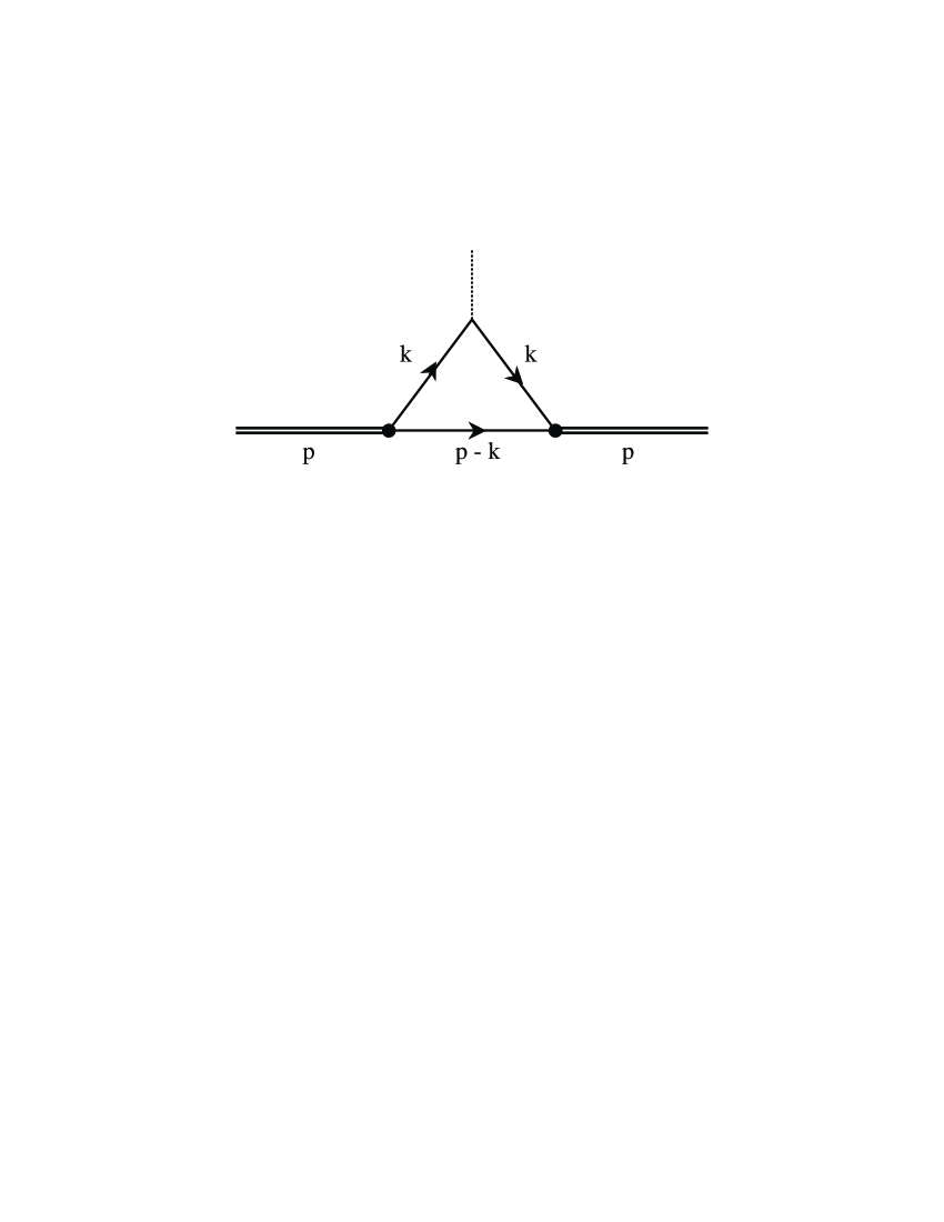
Figure 7: Diagram used in the calculation of the normalization factor of the kaon or scalar diquark is shown. (See the Appendix.)

References

- (1) T. Nakano et al., LEPS Collaboration, Phys. Rev. Lett. 91, 012002 (2003).
- (2) V.V. Barmin et al., DIANA Collaboration, Phys. At. Nucl. 66, 1715 (2003).
- (3) C. Alt et al., NA49 Collaboration, Phys. Rev. Lett. 92, 042003 (2004).
- (4) A. Aktas et al., H1 Collaboration, Phys. Lett. B588, 17 (2004).
- (5) V. Kubarovsky et al., CLAS Collaboration, Phys. Rev. Lett. 92, 032001 (2004).
- (6) S. Stepanyan et al., CLAS Collaboration, Phys. Rev. Lett. 91, 252001 (2003).
- (7) J. Barth et al., SAPHIR Collaboration, Phys. Lett. B572, 127 (2003).
- (8) M. Abdel-Bary et al., COSY-TOF Collaboration, Phys. Lett. B595, 127 (2004).
- (9) S. Chekanov et al., ZEUS Collaboration, Phys. Lett. B591, 7 (2004).
- (10) M. I. Adamovich, WA89 Collaboration, hep-ex/0405042 v2.
- (11) S. Chekanov et al., ZEUS Collaboration, Phys. Lett. B610, 212 (2005).
- (12) R. Jaffe and F. Wilczek, Phys. Rev. Lett. 91, 23003 (2003); Eur. Phys. J. C33, S38 (2004).
- (13) A. Hosaka, hep-ph/0506138.
- (14) M. Karliner and H.J. Lipkin, Phys. Lett. B586, 303 (2004).
- (15) M. Karliner and H.J. Lipkin, Phys. Lett. B575, 249 (2003).
- (16) Hu Li, C.M. Shakin and Xiangdong Li, hep-ph/0503145 (to be published in Phys. Rev. C).
- (17) Hu Li, C.M. Shakin and Xiangdong Li, hep-ph/0504125.
- (18) J. Szweda, L.S. Celenza, C.M. Shakin and W.-D. Sun, Few-Body Systems 20, 93 (1996).
- (19) U. Vogl and W. Weise, Prog. Part. Nucl. Phys. 27, 195 (1991).
- (20) H.J. Lee, N.I. Kochelev and V. Vento, Phys. Lett. B610, 50 (2005).
- (21) Zhi-Gang Wang, Wei-Min Yang and Shao-Long Wan, hep-ph/0504151.
- (22) Xiangdong Li and C.M. Shakin, Phys. Rev. D70, 114011 (2004).
- (23) V.N. Bannur, L.S. Celenza, Hung-He Chen, Shun-fu Gao and C.M. Shakin, Intl. J. Mod. Phys. A5, 1479 (1990).
- (24) M. Karliner and H.J. Lipkin, hep-ph/0506084.
- (25) Xiangdong Li and C.M. Shakin, Phys. Rev. C70, 068201 (2004).