Perfect Fluidity of the Quark Gluon Plasma Core
as Seen through its Dissipative Hadronic Corona

Abstract

The agreement of hydrodynamic predictions of differential elliptic flow and radial flow patterns with Au+Au data at $\sqrt{s_{NN}}=200$ GeV is one of the main lines of evidence suggesting the nearly perfect fluid properties of the strongly coupled Quark Gluon Plasma, sQGP, produced at RHIC. We study the sensitivity of this conclusion to different hydrodynamic assumptions on hadro-chemical and thermal freezeout after the sQGP hadronizes. We show that if chemical freezeout occurs at the hadronization time, as required to reproduce the observed hadron yields, then, surprisingly, the differential elliptic flow, $v_{2}(p_{T})$, for pions continues to increase with proper time in the late hadronic phase until thermal freezeout and leads to a discrepancy with the $v_{2}(p_{T})$ data. In contrast, if both hadro-chemical and thermal equilibrium are maintained past the hadronization point, then the mean transverse momentum per pion increases in a way that accidentally preserves $v_{2}(p_{T})$ from the sQGP phase in agreement with the data, but at the cost of the agreement with the observed hadronic yields. In order that all the data on (1) hadronic ratios, (2) radial flow, as well as (3) differential elliptic flow be reproduced, the sQGP core must expand with a minimal viscosity, $\eta\approx T_{c}^{3}$, that is however even greater than the viscosity, $\eta_{H}\approx T/\sigma_{H}$, of its hadronic corona. However, because of the large entropy density difference of the two phases of QCD matter, the larger viscosity in the sQGP phase leads to nearly perfect fluid flow in that phase while the smaller entropy density of the hadronic corona strongly hinders the applicability of Euler hydrodynamics in that phase. The “perfect fluid” property of the sQGP is thus not due to a sudden reduction of the viscosity at the critical temperature $T_{c}$, but to a sudden increase of the entropy density of QCD matter and is therefore an important signature of deconfinement.

I Introduction

One of the most intriguing experimental findings at the Relativistic Heavy Ion Collider (RHIC) in Brookhaven National Laboratory (BNL) is the large magnitude of the elliptic flow parameter $v_{2}$ Ackermann:2000tr ; Adcox:2002ms ; Back:2002gz in comparison with the smaller values observed at lower collision energies (for results at Super Proton Synchrotron (SPS) energies, see Refs. Alt:2003ab ; Agakichiev:2003gg ; Aggarwal:2004ub ). The magnitude of $v_{2}$ and in particular its transverse momentum $p_{T}$ and mass $m$ dependences at RHIC were found to be close to predictions based on ideal, non-dissipative hydrodynamics simulations around midrapidity ($\mid\eta\mid\mbox{\raisebox{-2.58334pt}{$\stackrel{{\scriptstyle<}}{{\sim}}$}}\>1$), in the low transverse momentum region ($p_{T}\mbox{\raisebox{-2.58334pt}{$\stackrel{{\scriptstyle<}}{{\sim}}$}}\>1$ GeV/$c$), and up to semicentral collisions ($b\mbox{\raisebox{-2.58334pt}{$\stackrel{{\scriptstyle<}}{{\sim}}$}}\>5$ fm) Kolb:2000fh ; Hirano:2001eu . This result has led to the recent BNL announcement BNL about the discovery of the near perfect fluidity of the strongly coupled/interacting quark gluon plasma (sQGP) Lee:2005gw ; Gyulassy:2004zy ; Shuryak:2004cy produced in ultra-relativistic nuclear reactions at RHIC.

Until RHIC data, “perfect fluidity” was never observed nor expected to apply theoretically in high energy hadronic or nuclear reactions due to nonvanishing viscous dissipation namiki . Especially, since the discovery of asymptotic freedom in QCD, the prevailing paradigm has been the expectation of large viscosities in a weakly coupled/interacting QGP (wQGP) at very high densities. In addition, it is well established Stoecker:2004qu that the hadronic resonance gas phase of QCD matter is highly dissipative. The discovery of elliptic flow at RHIC consistent with nearly perfect fluidity is therefore an experimental and theoretical surprise. Hence a new name, sQGP, has been adopted to characterize the observed strong coupling properties of the QGP near the critical temperature $T_{c}\sim$ 160–170 MeV that keep viscous effect to a minimum at RHIC.

In this paper, we present the case for the following physical interpretation of RHIC data based on current hydrodynamic analyses: (1) the high density core part of matter produced in relativistic heavy ion collisions, i.e. the sQGP, must expand as a nearly perfect fluid despite of its higher viscosity, (2) the perfect fluidity of the sQGP core is a consequence from a large jump of the entropy density at the critical temperature, $T_{c}$, i.e. deconfinement, and not from some anomalous reduction of its viscosity, (3) viscous effects on its hadronic corona are necessarily large despite its smaller viscosity, and (4) ideal inviscid hydrodynamics should not be applied to the hadronic corona which requires a nonequilibrium transport description.

In Sec. II, we discuss why we expect a surprising monotonic increase of the viscosity of QCD matter through the critical temperature and emphasize the important role played by the rapidly varying viscosity to entropy ratio in connection with perfect fluidity of the sQGP phase. In Sec. III, we discuss different assumptions for the hadronic matter in the hydrodynamic models to clarify what are open issues in the current hydrodynamic approaches. In Sec. IV, the time evolution of the transverse energy per particle is discussed. The mean transverse energy is found to be the key to distinguish the model assumptions in the hadron phase. Results from the hydrodynamic simulations are reviewed in Sec. V. We will show how the perfect fluid description for the hadronic matter in chemical equilibrium in the conventional hydrodynamic simulations leads to accidental reproduction of $p_{T}$ spectrum and $v_{2}(p_{T})$. In order to understand analytically the role of chemical freezeout on the transverse dynamics, we employ a blast wave model and give a dynamical meaning to this model in Sec. VI. Finally, summary of this study and an outlook are presented in Sec. VII.

II Viscosity and Entropy in QCD

Weak coupling perturbative QCD (pQCD) estimates Hosoya:1983xm ; Danielewicz:1984ww ; Thoma:1991em of the viscosity of a wQGP were based on basic kinetic theory relations

$$\eta_{\mathrm{wQGP}} \approx \frac{4}{15}\epsilon_{\mathrm{SB}}(T)\lambda_{\mathrm{tr}}\approx\frac{1}{5}\frac{T}{\sigma_{\mathrm{tr}}}\frac{s_{\mathrm{SB}}(T)}{n_{\mathrm{SB}}(T)},$$

$$\frac{\eta_{\mathrm{wQGP}}}{s_{\mathrm{SB}}} \approx \frac{T\lambda_{\mathrm{tr}}}{5}$$ (1)

where (in $\hbar=c=k_{B}=1$ units), $\epsilon_{\mathrm{SB}}(T)=3P_{\mathrm{SB}}(T)=\frac{3}{4}Ts_{\mathrm{SB}}(T)\approx 3Tn_{\mathrm{SB}}(T)\approx K_{\mathrm{SB}}T^{4}$ is the energy density, pressure, entropy density, and number density of an ideal Stefan-Boltzmann (SB) gas of quarks and gluon characterized by the constant $K_{\mathrm{SB}}=\frac{\pi^{2}}{30}[2(N_{c}^{2}-1)+\frac{7}{8}12N_{f}]\sim 12$–15 for $N_{c}=3,N_{f}=2$–3. The key microscopic dynamical quantity in Eq. (II) is the transport mean free path $\lambda_{\mathrm{tr}}=1/(n_{\mathrm{SB}}\sigma_{\mathrm{tr}})$ which is controlled in pQCD by the Debye screened transport cross section Danielewicz:1984ww ; Molnar:2001ux

$$\sigma_{\mathrm{tr}} = \int d\sigma_{\mathrm{el}}\;\sin^{2}\theta_{\mathrm{cm}}$$ (2)

$$= \frac{8\pi\alpha_{s}^{2}}{\hat{s}}(1+z)\left[(2z+1)\ln\left(1+\frac{1}{z}\right)-2\right]\;\;,$$

where $z=\mu^{2}/\hat{s}$ and $\hat{s}\approx 17T^{2}$ is the mean partonic Mandelstam variable. Perturbatively, the screening mass squared varies as $\mu^{2}\approx 4\pi\alpha_{s}T^{2}$. For numerical estimates we take $\alpha_{s}(T)\approx 4\pi/[18\ln(4T/T_{c})]$, so that $\alpha_{s}(T_{c})\sim 0.5$. In the range $T_{c}<T<5T_{c}$ ($0.5>\alpha_{s}(T)>0.23$), the perturbative transport cross section $\sigma_{\mathrm{tr}}<2$ mb remains much smaller than typical hadronic cross sections $\sigma_{H}\sim 10-20$ mb Danielewicz:1984ww ; Gavin:1985ph ; Muronga:2003tb .

An important dimensionless measure of how imperfect or dissipative a fluid may be given by the ratio of viscosity to entropy density, $\eta/s$ noteoncausal . This is most easily seen via the Navier-Stokes equation in (1+1)-dimensional boost invariant hydrodynamics Hosoya:1983xm ; Danielewicz:1984ww ; Gavin:1985ph . In the perfect (Euler) fluid limit, the proper energy density decreases with proper time, $\tau$, due to longitudinal expansion $dV=\pi R^{2}d\tau$ and $PdV$ work via $d\epsilon/d\tau=-(\epsilon+P)/\tau=-sT/\tau$ with a solution $T=T_{0}(\tau_{0}/\tau)^{1/3}$ for massless particles Bjorken:1982qr . However, shear and bulk viscosity reduce the ability of the system to perform useful work by adding a term $(4\eta/3+\zeta)/\tau^{2}$ to the right hand side. Neglecting bulk viscosity, $\zeta$, that vanishes in equilibrium for massless partons, $d\epsilon/d\tau=-(sT/\tau)[1-4(\eta/s)/3T\tau]$. This shows that for the earliest times consistent with the uncertainty principle Danielewicz:1984ww , $\tau\sim 1/3T$, the cooling of the plasma due to both expansion and work is canceled if $\eta/s>1/4$. The ability of the system to convert internal energy into collective flow is thus severely impaired at early times if $\eta/s$ and $\zeta/s$ are not very small. In fact, in order to reproduce the observed elliptic flow at RHIC, numerical solutions to covariant parton transport equation Molnar:2001ux and blast wave analysis with viscous corrections Teaney:2003pb showed that $\eta/s$ had to be less than about 0.2 during the first 3 fm/$c$.

The viscosity to entropy ratio in the weakly coupled QCD plasma on the other hand is

$$\left(\frac{\eta}{s}\right)_{\mathrm{wQGP}}=\frac{3}{5}\frac{T}{\sigma_{\mathrm{tr}}}\frac{1}{K_{\mathrm{SB}}T^{3}}\approx\frac{0.071}{\alpha_{s}(T)^{2}\ln[1/\alpha_{s}(T)]}$$ (3)

This ratio is not small ($\eta/s=0.35,0.48,0.58,0.66$ for $T/T_{c}=1,1.5,2.0,2.5$) indicating that the wQGP is expected to be a rather “poor fluid” with large dissipative corrections.

The analytic dependence on $\alpha_{s}$ in Eq. (3) reproduces well the approximate temperature dependence implied by Eq. (2) if we assume the perturbative variation of the screening scale $\mu$. Lattice QCD data Kaczmarek:1999mm indicate that $\mu\approx$ (2.0–2.5)$T$ is not far from the perturbative estimate extrapolated into the physical $g>1$ region and that $\alpha_{s}(T)<0.5$ above $T_{c}$ is also reasonable. However, the underlying simple gas kinetic approximation for the viscosity is only rigorously valid in the $g\ll 1$ region.

Formally, by increasing $\alpha_{s}>0.5$, it would seem that the right hand side of Eq. (3) could be made to be as small as we like if we ignore the $\ln(1/\alpha_{s})$ singularity. However, by the Heisenberg uncertainty principle, the transport mean free path cannot be localized to less than $\Delta x\sim 1/\langle p\rangle\sim 1/3T$. This leads to a quantum kinetic lower bound on the viscosity for ultrarelativistic gases Danielewicz:1984ww :

$$\frac{\eta}{s_{\mathrm{SB}}}\mathrel{\lower 3.87495pt\hbox{$\stackrel{{\scriptstyle\displaystyle>}}{{\sim}}$}}\frac{1}{15}\;$$ (4)

with an undetermined multiplicative factor on the order of unity.

A special quantum field theoretic determination of a viscosity lower bound was found recently for infinitely coupled supersymmetric Yang-Mills (SYM) gauge theory using the Anti de-Sitter Space/Conformal Field Theory (AdS/CFT) duality conjecture Kovtun:2004de :

$$\left(\frac{\eta}{s}\right)_{\mathrm{SYM}}=\frac{1}{4\pi}\;\;.$$ (5)

This bound is obtained in the dual $N_{c}=\infty$ and $g^{2}N_{c}=\infty$ limits of the special ${\cal N}=4$ conformal SYM schalm . It is interesting to note that this analytic SYM bound is close to the simple kinetic theory uncertainty principle bound in Eq. (4). It has been conjectured Kovtun:2004de that $1/4\pi$ in Eq. (5) is the universal minimal viscosity to entropy ratio even for QCD. In that case, the viscosity of the sQGP could be up to a factor of $\sim 1/2\pi$ smaller than of a wQGP. It is then tempting to conclude that the sQGP must have anomalously small viscosity if perfect fluid behavior is observed. However, as we show below, the sQGP viscosity is actually very close to that of ordinary hadronic matter just below $T_{c}$.

To develop this argument further, we first digress to recall that the entropy density in the $N_{c}\gg 1,g^{2}N_{c}\gg 1$ limits of ${\cal N}=4$ SYM is given by Gubser:1998nz

$$s_{\mathrm{SYM}}=\left[\frac{3}{4}+\frac{0.6}{(g^{2}N_{c})^{3/2}}+O\left(\frac{1}{N_{c}^{2}}\right)\right]\frac{4}{3}K_{\mathrm{SYM}}T^{3}\;\;.$$ (6)

where the Stefan-Boltzmann constant for ${\cal N}=4$ SYM is $K_{\mathrm{SYM}}={\pi^{2}(N_{c}^{2}-1)}/{2}\approx 39.5$ is about 3 times greater than $K_{\mathrm{SB}}$ of our QCD world schalm . What is especially remarkable about Eq. (6) is that, at infinitely strong coupling, the entropy density is only reduced by $\sim 25\%$ from its non-interacting SB value. On the other hand, the viscosity in this extreme limit is reduced about an order of magnitude from the weak coupling value and limited only by the quantum (Heisenberg uncertainty) bound on the effective scattering rate. Current lattice data on the QCD viscosity near $T_{c}$ Nakamura:2004sy are with large numerical error bars between these weak and super strong coupling limits but the relatively small deviation of the lattice entropy density from the SB limit is consistent with Eq. (6).

Figure 1: Illustration of the approximately monotonic increase of absolute value of the shear viscosity with temperature. The kink shown at $T_{c}$ is expected to be smeared out by the $\Delta T_{c}/T_{c}\sim 0.1$ width of the QCD cross-over transition. The solid blue curve shows $\eta(T<T_{c})=T/\sigma_{H}$ for a HRG followed by the more rapid increase of the viscosity in the sQGP phase with $\eta_{\mathrm{sQGP}}\approx\eta_{\mathrm{SYM}}\equiv K_{\mathrm{SB}}T^{3}/4\pi\approx T^{3}$. The horizontal line shows that near $T_{c}$, $\eta\approx\eta_{c}\equiv T_{c}^{3}$. At high $T\gg T_{c}$ asymptotic freedom leads to an even more rapid growth of viscosity as the sQGP evolves gradually into the weakly coupled wQGP. In this figure, $w=1$ in Eq. (10) is taken to emphasize the possibility that the highly viscous but nearly“perfect fluid” sQGP may become an ordinary “viscous fluid” already for $T\mathrel{\lower 3.87495pt\hbox{$\stackrel{{\scriptstyle\displaystyle>}}{{\sim}}$}}2T_{c}$.

Figure 2: Illustration of the rapid variation of the dimensionless ratio of the shear viscosity, $\eta(T)$, to the entropy density, $s(T)$. The sharp discontinuity illustrated is not due to a rapid change of the transport coefficient (see Fig. 1) but to the rapid increase of the entropy density in QCD near $T_{c}$. As in Fig. 1, we expect the discontinuity to be smeared into a rapid drop within $\Delta T_{c}/T_{c}\sim 0.1$. Solid (dashed) blue curve illustrates the change of $\eta/s$ of a HRG with $c_{H}^{2}=1/3$ (1/6), $s_{Q}/s_{H}=10$ (3) into an approximate “perfect fluid” sQGP at $T_{c}$. The red long dashed curve is $(\eta/s)_{\mathrm{SYM}}=1/4\pi$. At $T\gg T_{c}$ asymptotic freedom gradually transforms the sQGP into an ordinary viscous fluid wQGP (green), here shown for $w={\textstyle\frac{1}{2}},1$.

The AdS/CFT lower bound (5) together with the assumed universal $3/4$ reduction of the SB entropy density implies that the absolute value of the sQGP viscosity at $T_{c}$ would be

$$\eta_{\mathrm{sQGP}}(T)\approx\eta_{\mathrm{SYM}}(T)=\frac{K_{\mathrm{SB}}T^{3}}{4\pi}\approx T_{c}^{3}\left(\frac{T}{T_{c}}\right)^{3}$$ (7)

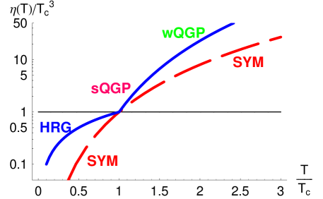
where we used a fact that for QCD $K_{\mathrm{SB}}\approx 12$–15 is accidentally close to $4\pi$. The monotonic increase of $\eta_{\mathrm{SYM}}(T)$ is illustrated by the dashed curve in Fig.1.

The effective transport cross section via Eq. (II) at $T_{c}\sim 160$ MeV is in this case

$$\sigma_{\mathrm{tr}}^{c}\approx\frac{4}{5}\frac{T_{c}}{\eta_{c}}\sim 12\;{\rm mb}\;\;.$$ (8)

Here $\eta_{c}\equiv T_{c}^{3}=0.106$ GeV/fm² at $T_{c}=0.16$ GeV. See Ref. Peshier:2005pp for an independent estimate of the transport cross section in the sQGP phase leading to similar $\sigma_{\mathrm{tr}}(T)$ near $T_{c}$.

While there is no consensus yet on what physical mechanisms could enforce the minimal viscosity bound in the sQGP Molnar:2001ux ; Shuryak:2003xe ; Xu:2004mz , we take as empirical fact that the sQGP viscosity must be close (within a factor of two) to the minimal (uncertainty) bound, Eq. (7). Our central assumption is that local thermal equilibrium is maintained in the sQGP core with minimal dissipative deviations and with the equation of state and hence speed of sound as predicted by QCD. Alternate scenarios, with arbitrary equations of state with higher speed of sound that in principle could compensate the higher dissipation and viscosity in a wQGP will not be considered here. In this connection we also emphasize the importance of fixing sQGP initial conditions with Color Glass Condensate or saturating gluon distributions constrained by the global entropy observables Gyulassy:2004zy ; Hirano:2004rs . With fixed initial conditions and equation of state, the remaining degrees of dynamical freedom are reduced to the dissipation corrections discussed in this section for the sQGP phase and the dynamical constraints on its dissipative hadronic corona discussed in the subsequent sections.

Note that the effective transport cross section in the sQGP $\sigma_{\mathrm{tr}}^{c}$ just above $T_{c}$ is remarkably close to the hadron resonance gas transport cross section just below $T_{c}$ Gavin:1985ph ; Muronga:2003tb . However, due to the $1/T^{2}$ scaling at $T\sim 2T_{c}$, the effective transport cross section in the sQGP would already drop to $\sim 3$ mb while preserving the (uncertainty principle) lower bound Eq. (5).

In contrast to the novel sQGP phase above $T_{c}$, for $T<T_{c}$, matter is well known to be in the confined hadron resonance gas (HRG) phase where the kinetic theory viscosity Danielewicz:1984ww ; Gavin:1985ph is

$$\eta_{\mathrm{HRG}}\approx\frac{T}{\sigma_{H}}\approx\eta_{c}\frac{T}{T_{c}}\;\;,$$ (9)

as illustrated by the solid curve below $T_{c}$ in Fig. 1. Because the hadronic transport cross sections are typically $\sigma_{H}\sim 10-20$ mb, the combination of Eqs. (7) and (9) shows that we should not expect a large variation of the absolute value of the matter viscosity across $T_{c}$ if the minimal $\eta/s$ holds above $T_{c}$. In Ref. Gavin:1985ph , Gavin found that for a pion gas with P-wave $\rho$ and D-wave $f^{0}$ resonance interactions, the thermal averaged transport cross section and viscosity from his Fig. 3 are $(\eta/\eta_{c},\sigma_{H}[\mathrm{mb}])\sim(0.66,20),~{}(0.9,17),~{}(1.1,15)$ for $T=180,~{}160,~{}140$ MeV. In Ref. Muronga:2003tb , Muronga used the UrQMD resonance gas Monte Carlo to compute $\eta(T)/\eta_{c}\sim 0.75,~{}1.1,~{}1.9$ for $T=0.14,~{}0.16,~{}0.18$ GeV. In both studies Gavin:1985ph ; Muronga:2003tb numerical estimates are thus consistent with Eq. (9) for $T<T_{c}$. For nonvanishing baryon density, see recent estimates in Ref. Muroya:2004pu .

In the sQGP phase, the minimal viscosity, Eq. (7), is predicted to grow cubically with $T$ beyond $T_{c}$. However, at $T\gg T_{c}$ asymptotic freedom predicts that it would grow even more rapidly as the sQGP transforms gradually into a wQGP. An interpolation formula between these phases can be constructed as

$$\eta(T)\approx T_{c}^{3}\left\{\begin{array}[]{ll}(T/T_{c})^{1},&T<T_{c}\\ (T/T_{c})^{3}[1+w(T)\ln(T/T_{c})]^{2},&T>T_{c}\end{array}\right.$$ (10)

The extra squared logarithmic growth of the viscosity at $T\gg T_{c}$ is expected from Eq. (3). To be consistent with the perturbative wQGP at $T\gg T_{c}$ one should take

$$\frac{w^{2}(T\gg T_{c})}{4\pi}=\frac{9\beta_{0}^{2}}{80\pi^{2}K_{\mathrm{SB}}}\frac{1}{\ln 1/\alpha_{s}(T)}\;\;.$$ (11)

With $K_{\mathrm{SB}}=12$–15 and $\beta_{0}=11-2N_{f}/3\sim 9$–10, a possible scenario may be that $w\sim 1$ already near $T_{c}$. This possibility is shown in Fig. 1 by the solid curve above $T_{c}$ which would imply sQGP$\rightarrow$ wQGP already above $\sim(2-3)T_{c}$. In fact, current lattice data on the evolution of screening scales in the QGP phase suggest that hadronic scale correlations may persist only up to $T\sim 3T_{c}$ Asakawa:2003re ; Datta:2003ww . A value $w(T>2T_{c})\sim 1$, is also not inconsistent with current lattice results Nakamura:2004sy . We note that future measurements of elliptic flow in A+A collisions at LHC with $\sqrt{s_{NN}}=5500$ GeV will be able to test experimentally if such a precocious onset of dissipative wQGP dynamics occurs.

The approximate continuity of the viscosity across $T_{c}$ indicated in Fig. 1 is to be understood to hold within a factor on the order of unity. What changes rapidly at $T_{c}$ is not the viscosity of QCD matter but rather its entropy density due to the deconfinement of the quark and gluon degrees of freedom.

For a hadronic resonance gas charactered by a speed of sound $c_{H}^{2}$, the entropy density $s(T)=s_{H}(T/T_{c})^{1/c_{H}^{2}}$ with decreasing temperature decreases much more rapidly than does the viscosity for typical $c_{H}^{2}\sim 1/6$–1/3. Just beyond $T_{c}$ –possibly only up to several times $T_{c}$– it is postulated that the sQGP phase may exist with $\eta/s<0.2$ but with viscosity close to ideal gas.

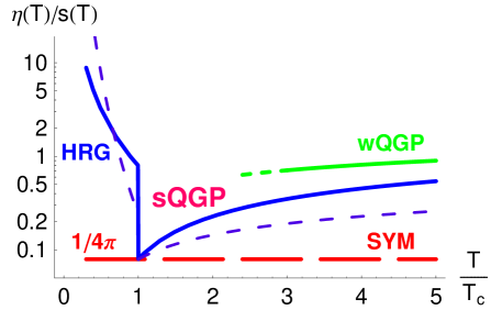
Summarizing the discussion up to now, we expect that $\eta$ varies smoothly near $T_{c}$ as in Fig. 1 while the ratio $\eta/s$ may have a significant discontinuity due to the rapid onset of deconfinement as a function of $T$ as shown in Fig. 2. We therefore propose the following interpolation formula for the temperature dependence of the $\eta/s$ ratio with a $T$ independent constant $w$

$$\frac{\eta(T)}{s(T)}\approx\frac{1}{4\pi}\left\{\begin{array}[]{ll}\left(\frac{s_{Q}}{s_{H}}\right)\left(\frac{T}{T_{c}}\right)^{1-1/c_{H}^{2}},&T<T_{c}\\ \left[1+w\;\ln(T/T_{c})\right]^{2},&T>T_{c}\end{array}\right.$$ (12)

with the negative discontinuity

$$\left[\frac{\eta}{s}\right]_{T_{c}}=\left.\frac{\eta(T_{c})}{s(T_{c})}\right|_{Q}-\left.\frac{\eta(T_{c})}{s(T_{c})}\right|_{H}=-\frac{1}{4\pi}\left(\frac{s_{Q}}{s_{H}}-1\right)\;\;.$$ (13)

We illustrate Eq. (12) in Fig. 2. Note that it is the entropy jump $s_{Q}/s_{H}\sim 3$–10 that causes a drop of $\eta/s$ across $T_{c}$. Since the HRG$\rightarrow$ sQGP transition with dynamical quarks appears from the lattice QCD to be only a rapid crossover, the discontinuity is understood to be spread out over a temperature range $\Delta T_{c}/T_{c}\sim 0.1$.

III Imperfect Fluidity of the Hadronic Corona

In the last section we presented the case that the $\eta/s$ ratio may be small enough above $T_{c}$ in the sQGP core for perfect fluidity to arise during the critical first $\sim 3$ fm/$c$, while the spatial azimuthal asymmetry of the matter produced in non-central reactions is large enough to induce collective elliptic flow. However, during the subsequent $\sim 10$ fm/$c$ evolution after hadronization of the sQGP core, the whole system evolves as HRG corona. In the HRG, $\eta/s$ is too high for local equilibrium to be maintained due to its small entropy density compared with sQGP. Nevertheless, the data on $v_{2}(p_{T})$ seem to agree very well with some hydrodynamic predictions based on the assumption that local equilibrium is maintained until thermal freeze-out. However, various assumptions about the hadro-chemical evolution are known to lead to significantly different predictions for the differential elliptic flow. In this section we focus on the question of the validity of the application of hydrodynamics to analyze the entire evolution in A+A at RHIC.

The key problem that we now address is the role of final state hadronic interactions in possibly modifying conclusions inferred about the prefect fluidity of the sQGP core. In order that the sQGP elliptic flow signature of perfect fluidity survives during the evolution through the extended hadronic “corona” we must study how longitudinal flow, transverse radial flow, as well as the elliptic deformation of the transverse flow may evolve in hadronic matter.

Several puzzling features suggest the importance of investigating more closely the distortions that can be caused by final state hadronic interactions involving hadro-chemical and thermal freezeout. In ideal hydrodynamics it is well known that while the central rapidity region is well reproduced by hydrodynamics, this is not the case in forward/backward rapidity regions Hirano:2001eu . Hydrodynamics also strongly overestimates $v_{2}$ at energies below $\sqrt{s_{NN}}=$200 GeV as well as in the most peripheral collisions where initially a larger fraction of the transverse elliptic interaction region starts out in the hadronic phase. All these data point to the fact that the dynamics in the hadronic corona is not at all ideal.

Another important issue in ideal hydrodynamics as well as in other dynamical models is the so-called HBT puzzle Heinz:2002un . In spite of the apparent success of hydrodynamic description for elliptic flow, hydrodynamics fails to reproduce the experimental data of the HBT radii Adler:2001zd ; Adcox:2002uc ; Back:2004ug . The best current description of hadron freezeout consistent with the HBT puzzle involves an assumption of a highly dissipative resonance gas dynamics and transport Lin:2002gc .

As compiled in Fig. 20 in Ref. Adcox:2004mh , some hydrodynamic results reproduce neither $v_{2}(p_{T})$ nor $p_{T}$ spectrum. This immediately raises the following two questions:

(Q1) Are hydrodynamic results consistent with each other at RHIC energies? What assumptions lead to the differences among hydrodynamic predictions?

(Q2) How robust is the statement that hydrodynamic description at RHIC data is good at low $p_{T}$?

The differences arise from the treatment of hadron phase dynamics. The treatment of the sQGP phase is essentially the same in all approaches so far: Parton chemical equilibrium and inviscid hydrodynamics are assumed in the sQGP phase. There are, however, three generic classes of approaches to the evolution of the hadronic corona in the literature.

Chemical equilibrium model (CE). Most of the hydrodynamic calculations so far are based on the assumption that the hadron phase is a perfect fluid in both hadro-chemical and thermal equilibrium. With this assumption, the centrality, transverse momentum, and/or (pseudo)rapidity dependences of elliptic flow are studied Kolb:2000fh ; Hirano:2001eu . However, it is known that the yields of heavy hadrons (essentially all hadrons except for pions) are smaller in CE than data since the numbers of particle are counted on the hypersurface at thermal freezeout within this approach. At relativistic collisional energies, thermal freezeout temperature $T^{\mathrm{th}}$ is smaller than chemical freezeout temperature $T^{\mathrm{ch}}$ Heinz:1997za ; Shuryak:1997xb . So the numbers of heavy particles are suppressed due to the Boltzmann factor and, eventually, lead to discrepancy from the data. CE therefore fails to account for the observed particle abundance systematics Braun-Munzinger:2003zd .

Partial chemical equilibrium model (PCE). In Refs. Arbex:2001vx ; Hirano:2002ds ; Teaney:2002aj ; Kolb:2002ve , chemical freezeout being separated from thermal freezeout is taken into account in the hydrodynamic simulations toward simultaneous reproduction of particle ratios and particle spectra. Below $T^{\mathrm{ch}}$, one introduces chemical potential for each hadron associated with the conserved number. Inelastic processes only through strong interactions are supposed to be equilibrated in the hadron phase, e.g. $\mu_{\rho}=2\mu_{\pi}$, $\mu_{\Delta}=\mu_{N}+\mu_{\pi}$, and so on. Note that the conserved pion number within this approach is $\tilde{N}_{\pi}=N_{\pi}+\sum_{R}b_{R}N_{R}$. Here $b_{R}$ is the effective branching ratio and $N_{i}$ is the number of $i$-th hadron Bebie:1991ij . For details, see Refs. Hirano:2002ds ; Teaney:2002aj ; Kolb:2002ve . This particular model does not reproduce $v_{2}(p_{T};m)$ nor $p_{T}$ spectra at RHIC as shown in Fig. 20 in Ref. Adcox:2004mh . Note that a model is called “chemical freezeout (CFO)” when the number of hadrons $N_{i}$ instead of $\tilde{N}_{i}$ is conserved. This means even inelastic scatterings through strong interaction cease to happen.

Hadronic cascade model (HC). One can utilize a hadronic cascade model just after the phase transition between the QGP and hadron phases Bass:2000ib ; Teaney:2000cw . This approach dynamically describes both chemical and thermal freezeouts without assuming explicit freezeout temperatures. Viscous effects are effectively taken into account through the non-zero mean free path among the particles (see, e.g. Eqs. (II) and (9)).

Table 1: Summary of hydrodynamic results. Hydrodynamic results of $v_{2}(p_{T})$ and $p_{T}$ spectra for pions and protons are compiled in Fig. 20 in Ref. Adcox:2004mh . CE, PCE, and HC stand for, respectively, chemical equilibrium, partial chemical equilibrium, and hadronic cascade. Thermal freezeout temperature is assumed to be chosen to reproduce particle spectra in the model CE. Note that the model CE can reproduce the shape of $dN/p_{T}dp_{T}$ for protons, not its yield.

Observables	model CE	model PCE	model HC
$v_{2}(p_{T};m)$	yes	no	yes
$dN/p_{T}dp_{T}$	yes	no	yes
ratios	no	yes	yes

Hydrodynamic results from the above three classes of hadro-dynamical models are summarized in Table 1. For reviews of hydrodynamic results at the RHIC energies, see also Huovinen:2003fa ; Kolb:2003dz ; Hirano:2004ta . As long as the space-time evolution of the hadron phase is concerned, the approach HC seems to be the most realistic one among the three classes. The second best model should be the model PCE from the experimental data of particle ratios and spectra. The models CE and HC reproduce $v_{2}(p_{T})$ for pions and protons in low $p_{T}$ regions, whereas the model PCE fails. The failure of PCE for $v_{2}(p_{T})$ is particularly perplexing since the spatial azimuthal asymmetry is mostly gone by the time hadronization is competed. In the following sections, we shall show why the differences between the models CE and PCE appears and why the result from the perfect fluid model CE eventually looks similar to the one from the highly dissipative model HC. The key quantities to understand these differences are found to be the temporal behavior of the mean transverse momentum/energy and the ratio of the particle number to the entropy.

IV Temporal behavior of transverse energy

In this section, we briefly review the time evolution of total transverse energy and transverse energy per particle in relativistic heavy ion collisions within a framework of the Bjorken solution for longitudinal expansion Bjorken:1982qr .

Assuming the Bjorken scaling solution, the time evolution of the entropy density is represented by $s(\tau)=s_{0}\tau_{0}/\tau$. Here $s_{0}$ is the initial entropy density and $\tau_{0}$ is the initial time. As long as a perfect fluid is considered, the entropy per unit rapidity is conserved

$$\frac{dS}{dy} = \int d^{2}x_{\perp}\tau s(\tau)=A_{\perp}\tau_{0}s_{0},$$ (14)

where $A_{\perp}$ is the transverse cross section of a nucleus. Here we assume a smooth function for the equation of state (EOS). For EOS with $P=c_{s}^{2}\epsilon$ $(0<c_{s}^{2}<1/3)$, the time evolution of energy density becomes

$$\epsilon(\tau) = \epsilon_{0}\left(\frac{\tau_{0}}{\tau}\right)^{1+c_{s}^{2}}$$ (15)

where $\epsilon_{0}$ is the energy density at $\tau_{0}$. Thus the transverse energy per unit rapidity

$$\frac{dE_{T}}{dy} = \int d^{2}x_{\perp}\tau\epsilon(\tau)=A_{\perp}\epsilon_{0}\tau_{0}\left(\frac{\tau_{0}}{\tau}\right)^{c_{s}^{2}}$$ (16)

decreases with proper time due to $PdV$ work in spite of the conservation of entropy Gyulassy:1983ub ; Ruuskanen:1984wv . In the following discussion in this section, we consider three EOS models for pions and see time evolution of total transverse energy and transverse energy per pion.

Massless Pions. The number density $n$ is proportional to the entropy density $s$ for massless pions: $n=(d/\pi^{2})\zeta(3)T^{3}$, $s=d(4\pi^{2}/90)T^{3}$. Inserting $d=3$ and $\zeta(3)\sim 1.2$, one obtains $s\approx 3.6n$. From Eq. (14), the number of pions per unit rapidity $dN/dy$ is also conserved. Therefore the mean transverse mass, which is identical to the mean transverse momentum in the massless pion case, $\langle m_{T}\rangle=(dE_{T}/dy)/(dN/dy)\propto(dE_{T}/dy)$ decreases with $\tau$ from Eq. (16).

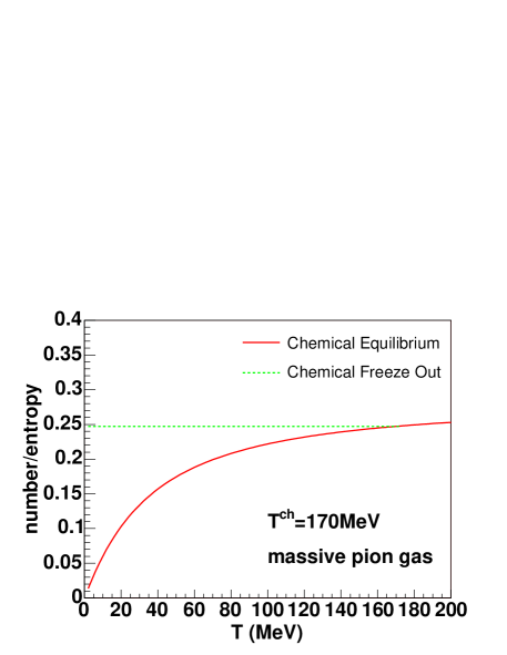
Massive Pions in Chemical Equilibrium. The proportionality between the number density and the entropy density is approximately valid only for ultra-relativistic particles ($T\gg m$). In relativistic heavy ion collisions, the typical temperature is around the order of the pion mass. So pions are no longer relativistic particles in this particular situation. The number density and the entropy density for pions are evaluated in the usual prescription of statistical physics. Thus the ratio of the number $N$ and the entropy $S$ increases with temperature due to the finite mass of pions as shown in Fig. 3. Note that the volume $V$ is canceled and that $N/S$ equals to the ratio of their densities $n/s$. Therefore $\langle m_{T}\rangle$ can increase with proper time (or with decreasing temperature of the system) even as $dE_{T}/dy=\langle m_{T}\rangle dN/dy$ decreases from Eq. (16). This “local reheating” can occur because the total transverse energy is distributed among a smaller number of pions at lower temperature. The resulting temporal behavior of $\langle m_{T}\rangle$ is determined through competition of how rapidly $dE_{T}/dy$ and $dN/dy$ decrease with proper time. As we will see in the next section, $\langle p_{T}\rangle$ increases with proper time in hydrodynamic simulations with chemical equilibrium EOS.

Figure 3: The ratio of number density and entropy density for massive pions. Solid (Dashed) line represents the ratio for chemical equilibrium (chemical freezeout). Chemical freezeout temperature is assumed to be $T^{\mathrm{ch}}=170$ MeV.

Chemically Frozen Massive Pions. When the system expands strongly, inelastic collisions can cease to happen. So one can think about a situation in which the system keeps only thermal equilibrium through elastic scattering. Analyses based on statistical models and blast wave models show that thermal freezeout temperature $T^{\mathrm{th}}$ is smaller than chemical freezeout temperature $T^{\mathrm{ch}}$ at AGS, SPS and RHIC energies. Moreover, $T^{\mathrm{ch}}$ is found to be close to the (pseudo)critical temperature $T_{c}$. This indicates that the hadron phase in relativistic heavy ion collisions is in thermal equilibrium, not in chemical equilibrium Heinz:1997za ; Shuryak:1997xb . Usually, the term “chemical equilibrium” is associated with a state equilibrated among a finite number ($>1$) of compositions in the system. Here we simply use the term “chemical freezeout” in spite of one hadronic species, i.e. pions. This means the number of pions per unit rapidity is fixed below $T^{\mathrm{ch}}$. The entropy is also conserved as long as a perfect fluid is considered, so the ratio of the number density and the entropy density is a constant of motion similar to the case for massless pions. It is interesting to mention that the entropy is not generated even in the evolution of chemically frozen fluids. Entropy production originates from the source term in the rate equation for chemical non-equilibrium processes. The number of hadron is, however, conserved after chemical freezeout. It is easy to show the conservation of entropy $\partial_{\mu}S^{\mu}=0$ from the conservation of energy and momentum $\partial_{\mu}T^{\mu\nu}=0$, where $T^{\mu\nu}=(\epsilon+P)u^{\mu}u^{\nu}-Pg^{\mu\nu}$, and the conservation of the number of hadrons $\partial_{\mu}N_{i}^{\mu}=0$. In this sense, one needs to distinguish “chemical freezeout” from “chemical non-equilibrium”. In the chemical non-equilibrium process, the system is approaching to chemical equilibrium state, i.e. the maximum entropy state through inelastic scattering. Entropy is certainly generated during this process. Contrary to this, chemical freezeout means that the system suddenly leaves from the chemical equilibrium state by keeping particle ratios due to the strong expansion.

Figure 3 shows comparison of the ratio of pion number $N$ and its entropy $S$ between chemical equilibrium EOS and chemically frozen EOS. Here chemical freezeout temperature is taken as being $T^{\mathrm{ch}}=170$ MeV. Similar to the massless pion case, $\langle m_{T}\rangle$ in the chemical freezeout case decreases with decreasing decoupling temperature. As long as the Bjorken scaling solution for longitudinal expansion is considered, transverse expansion does not spoil the above discussion: $PdV$ work done in the transverse direction is simply converted into the kinetic energy of fluid elements. The resultant slope of $p_{T}$ spectrum for pions should become softer at lower decoupling (thermal freezeout) temperature. Quantitatively, the $p_{T}$ slope is insensitive to the choice of $T^{\mathrm{th}}$ since $dE_{T}/dy\propto\tau^{-c_{s}^{2}}$ changes only gradually in the late stage. The universal behavior of the $p_{T}$ slope is already confirmed in the hydrodynamic simulations with chemically frozen (or partial chemical equilibrium) EOS Hirano:2002ds ; Kolb:2002ve and will be mentioned in the next section.

From the above consideration, the key quantity which governs the transverse dynamics, particularly the time evolution of mean transverse mass, within ideal hydrodynamics is found to be the ratio of the number $N$ and the entropy $S$. It is commonly expected that the behavior of the mean transverse energy/momentum is governed by the stiffness of the EOS. But it is not always true since the sound velocity of chemical freezeout EOS (or simply the slope of $P$ as a function of $\epsilon$) is almost the same as that of chemical equilibrium EOS as shown in Ref. Hirano:2002ds . Interestingly, whether the mean transverse energy increases or decreases with the proper time is governed by $N/S$ and the longitudinal work, not the stiffness of EOS. We will also mention these hydrodynamic results in the next section.

To summarize this section, $\langle m_{T}\rangle$ decreases with proper time for massless pions or chemically frozen massive pions, while it can increase for massive pions in chemical equilibrium. We emphasize here that these conclusions are obtained from quite basic assumptions: the first law of thermodynamics ($PdV$ work) and the Bjorken scaling solution.

V Results from Hydrodynamic Simulations

We compare the hydrodynamic results from the model PCE with the ones from the model CE with respect to the EOS, space-time evolution, $p_{T}$ spectra, and $v_{2}(p_{T})$. Hydrodynamic simulations have already been performed for Au+Au collisions at $\sqrt{s_{NN}}=130$ GeV and the essential results have already been obtained in Ref. Hirano:2002ds . In this section, we make an interpretation of these hydrodynamic results obtained so far. In particular, we emphasize that the temporal behavior of the mean $p_{T}$ is the key to understand the difference of the results between these two models. For further details of the hydrodynamic model, see also Ref. Hirano:2002ds .

V.1 Equation of state and space-time evolution

Chemical freezeout does not change EOS, i.e. pressure as a function of energy density $P(\epsilon)$, so much Hirano:2002ds ; Teaney:2002aj . This means that the difference of chemical composition in the hadron phase does not affect the space-time evolution of energy density significantly. However, at a fixed temperature, the energy density in chemically frozen (or partial chemical equilibrium) hadronic matter is considerably larger than the one for hadronic matter in chemical equilibrium. This is due to the fact that the large resonance population keeps in the system during the expansion after chemical freezeout and that the mass terms significantly contributes to the energy density. Therefore the space-time evolution of temperature field does change significantly while $P(\epsilon)$ remains essentially unchanged. The temperature of the chemically frozen system cools down more rapidly than that of the chemical equilibrium system. This leads to the reduction of life time of fluids, radial flow, and HBT radii ($R_{\mathrm{long}}$ and $R_{\mathrm{out}}$) Hirano:2002ds . Longitudinal size $R_{\mathrm{long}}$, which relates with the lifetime of a fluid through the gradient of longitudinal flow velocity $(dv_{z}/dz)^{-1}\approx\tau_{f}$ Makhlin:1987gm , can be interpreted by the effect of chemical freezeout on the life time of a fluid in hydrodynamics. Nevertheless, $R_{\mathrm{side}}$ and $R_{\mathrm{out}}$ are still inconsistent with data.

V.2 $p_{T}$ spectra and elliptic flow

In hydrodynamic simulations with chemical equilibrium, thermal freezeout temperature $T^{\mathrm{th}}$ is an adjustable parameter. In order to fix $T^{\mathrm{th}}$, one usually utilizes the experimental data of $p_{T}$ spectra for hadrons. Reduction of $T^{\mathrm{th}}$ leads to generation of additional radial flow. Generically, the resulting $p_{T}$ spectra at $T^{\mathrm{th}}=T_{1}$ becomes harder than the ones at $T^{\mathrm{th}}=T_{2}>T_{1}$ even though temperature, i.e. the inverse slope of the momentum distribution in the local rest frame decreases. Contrary to this behavior, when chemical freezeout is appropriately taken into account in hydrodynamic simulations, the $p_{T}$ slope becomes insensitive to $T^{\mathrm{th}}$ compared to the one in the model CE Hirano:2002ds .

Figure 4: Average transverse momentum for pions as a function of thermal freezeout temperature for the models CE (solid) and PCE (dashed).

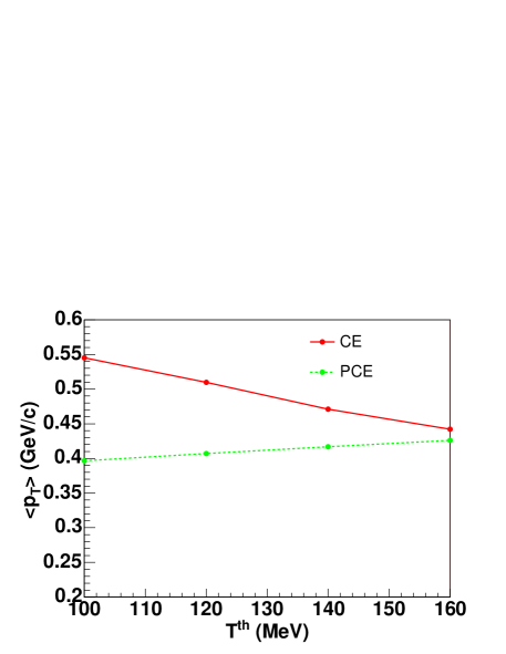
To confirm these behaviors, we perform hydrodynamic simulations again for a particular choice of impact parameter $b=5$ fm and see the average transverse momentum $\langle p_{T}\rangle$. Details of the hydrodynamic models used here can be found in Ref. Hirano:2002ds ; Hirano:2003pw . Figure 4 shows $\langle p_{T}\rangle$ for pions as a function of $T^{\mathrm{th}}$ at midrapidity $y=0$. In chemical equilibrium, $\langle p_{T}\rangle$ increases with decreasing $T^{\mathrm{th}}$. On the contrary, $\langle p_{T}\rangle$ gradually decreases with decreasing $T^{\mathrm{th}}$ when early chemical freezeout is taken into account. Even in the case that a full hydrodynamic simulation without boost invariant ansatz is performed and that the contribution from resonance decays is included, the temporal behavior of $\langle p_{T}\rangle$ as already discussed in Sec. IV is seen in Fig. 4. It should be emphasized here that increase of $\langle p_{T}\rangle$ in chemical equilibrium is a direct consequence of neglecting chemical freezeout in hydrodynamic calculations and, more definitely, of the experimental results of particle ratios. One has made full use of this unrealistic behavior to reproduce $p_{T}$ spectra at the cost of hadron ratios in the conventional hydrodynamic calculations.

Figure 5: $v_{2}$ for pions as a function of $T^{\mathrm{th}}$ for the models CE (solid) and PCE (dashed).

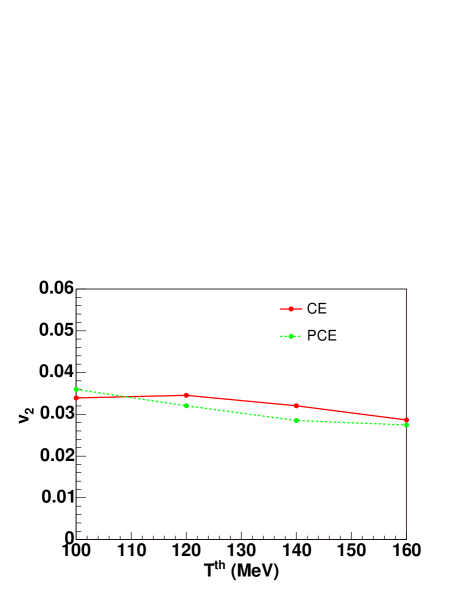
In chemical equilibrium, the slope of elliptic flow parameter $dv_{2}(p_{T})/dp_{T}$ for pions is insensitive to $T^{\mathrm{th}}$ and is consistent with the experimental data. See also Figs. 8 and 11 in Ref. Hirano:2002ds . This is apparently plausible since the elliptic flow is a self-quenching phenomenon and is sensitive to the early stage of the collisions Ollitrault:1992bk . On the other hand, $dv_{2}(p_{T})/dp_{T}$ for pions in the model PCE increases with decreasing $T^{\mathrm{th}}$ and is ended with overprediction of the experimental data when $T^{\mathrm{th}}$ is chosen so as to reproduce the proton $p_{T}$ spectrum and $v_{2}(p_{T})$ in the low $p_{T}$ region. This means that $v_{2}(p_{T})$ for pions varies in the late hadronic stage ($\tau\mathrel{\lower 3.87495pt\hbox{$\stackrel{{\scriptstyle\displaystyle>}}{{\sim}}$}}$ 10 fm/$c$).

We have to be careful in understanding the difference between integrated elliptic flow $v_{2}$ and differential elliptic flow $v_{2}(p_{T})$. $v_{2}$ reflects the momentum anisotropy of bulk matter, while $v_{2}(p_{T})$ represents how total $v_{2}$ distributes among various particles with different $p_{T}$. As shown in Fig. 5, the integrated $v_{2}$ varies only weakly with decrease of $T^{\mathrm{th}}$ (and hence proper time $\tau$) in both cases. This is consistent with the self-quenching picture of elliptic flow again.

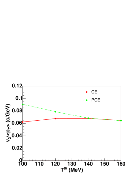
The slope of $v_{2}(p_{T})$, on the other hand, can be evaluated approximately by $dv_{2}(p_{T})/dp_{T}\approx v_{2}/\langle p_{T}\rangle$ since $v_{2}(p_{T})$ for pions is almost a linear function of $p_{T}$ noteonv2slope . In chemical equilibrium (CE), the moderate increase of $v_{2}$ ($\sim$13% increase as $T^{\mathrm{th}}$ decreases from 160 MeV to 100 MeV) is approximately canceled by the increase of $\langle p_{T}\rangle$ ($\sim$22% from 160 MeV to 100 MeV). Eventually, the ratio remains almost constant (or even decreases slightly) as shown in Fig. 6. The CE predictions for the differential elliptic flow work because without chemical freezeout the slope of $v_{2}(p_{T})$ stalls accidentally and reproduces the experimental data.

On the contrary, in PCE the numerator $v_{2}$ increases by $\sim$20% and the denominator $\langle p_{T}\rangle$ decreases by $\sim$10%. The resultant ratio $v_{2}/\langle p_{T}\rangle$ therefore increases with decreasing $T^{\mathrm{th}}$ as shown in Fig. 6. This is the reason why the slope of $v_{2}(p_{T})$ in PCE increases even in the late stage after the spatial azimuthal asymmetry has reversed sign.

It is now easy to understand why $v_{2}(p_{T})$ at the SPS energies is so close to the one at the RHIC energy (see, e.g. Fig. 17 in Ref. Adams:2005dq ). This is due to the correlated change of both $v_{2}$ and $\langle p_{T}\rangle$ from SPS to RHIC energies: The increase of the average $v_{2}$ is compensated for by the increase of $\langle p_{T}\rangle$. The slopes of $v_{2}(p_{T})$ therefore vary surprisingly weakly with the beam energy.

Figure 6: $v_{2}/\langle p_{T}\rangle$ for pions as a function of $T^{\mathrm{th}}$ for the models CE (solid) and PCE (dashed).

Summarizing the discussion, differential elliptic flow is sensitive to the late hadronic stage in ideal hydrodynamic calculations with early chemical freezeout since the slope of $v_{2}(p_{T})$ is determined by the mean $p_{T}$, i.e. radial flow. The apparent consistency of $v_{2}(p_{T})$ between RHIC data and results based on conventional CE hydrodynamic simulations is therefore fortuitous.

VI Analytic Approach

In order to understand the effect of chemical freezeout on the transverse momentum dependence of elliptic flow analytically, we employ the blast wave model discussed in Ref. Pratt:2004zq . In the framework of the blast wave model, one can choose the radial flow parameter and temperature independently to reproduce the slope of $p_{T}$ spectra. However, these two parameters are correlated in actual hydrodynamic simulations. After chemical freezeout, the mean $p_{T}$ decreases with decreasing $T^{\mathrm{th}}$, i.e. $d\langle p_{T}\rangle/dT>0$, as already discussed in the previous sections. On the contrary, the mean $p_{T}$ increases with decreasing $T^{\mathrm{th}}$, i.e. $d\langle p_{T}\rangle/dT<0$, in chemical equilibrium. So we can constrain the average flow velocity as a function of temperature through the condition $d\langle p_{T}\rangle/dT=0$. We call the obtained radial flow the critical radial flow, $v_{r}^{\mathrm{crit}}(T)$. The critical radial flow ensures that the mean $p_{T}$ is a constant of motion. Qualitatively, $v_{r}(T)<v_{r}^{\mathrm{crit}}(T)$ corresponds to the chemically frozen system, while $v_{r}(T)>v_{r}^{\mathrm{crit}}(T)$ corresponds to the system under chemical equilibrium. In the following in this section, we assume only pions which are dominant particles in a fluid element.

VI.1 Momentum Distribution

The invariant momentum spectrum is given by the Cooper-Frye formula Cooper:1974mv in the Boltzmann approximation:

$$E\frac{dN}{d^{3}p} = \frac{g}{(2\pi)^{3}}\int p^{\mu}d\sigma_{\mu}\exp\left(-\frac{p^{\mu}u_{\mu}-\mu}{T}\right).$$ (17)

Here $g$ is the degree of freedom, $d\sigma^{\mu}$ is the element of freezeout hypersurface. $p^{\mu}$ is the four momentum measured in the laboratory system. $\mu$ and $T$ are, respectively, chemical potential and temperature at freezeout. Four fluid velocity ($u^{\mu}u_{\mu}=1$) can be parametrized as

$$u^{\mu} = \cosh\rho(\cosh\eta_{f},\sinh\rho\cos\phi,\sinh\rho\sin\phi,\sinh\eta_{f}).$$

Here $\rho$ is the transverse rapidity and $\eta_{f}$ is the longitudinal rapidity which is to be identified with the space-time rapidity $\eta_{s}$ in the Bjorken boost invariant solution Bjorken:1982qr . One can also write $\cosh\rho=\sqrt{1+u_{\perp}^{2}}$ and $\sinh\rho=u_{\perp}$, respectively. Energy of a particle in the local rest frame becomes

$$p^{\mu}u_{\mu}=m_{T}\cosh(y-\eta_{f})\sqrt{1+u_{\perp}^{2}}-p_{T}u_{\perp}\cos(\phi_{p}-\phi).$$

Here $y$ is the momentum rapidity and $\phi_{p}$ is the azimuthal angle of the momentum. According to Ref. Pratt:2004zq , we also make the same ansatz $u_{\perp}(\phi)=u_{\perp}(1+\varepsilon\cos 2\phi)$ for azimuthal dependence of radial flow and take terms up to the first order in $\varepsilon$

$$p^{\mu}u_{\mu} = m_{T}\cosh(y-\eta_{f})\sqrt{1+u_{\perp}^{2}}\left[1+\frac{u_{\perp}^{2}}{1+u_{\perp}^{2}}\varepsilon\cos 2\phi\right]$$ (19)

$$- p_{T}u_{\perp}\cos(\phi_{p}-\phi)(1+\varepsilon\cos 2\phi).$$

Assuming the matter suddenly freezes out at $\tau_{f}$,

$$p^{\mu}d\sigma_{\mu}=EdV=m_{T}\cosh y\times rdrd\phi\tau_{f}d\eta_{s}.$$ (20)

Note that $u_{\perp}(\phi)$ is supposed to include all possible azimuthal anisotropic effects and that $\phi$ dependences of $T$ and $\mu$ are neglected as in the hydrodynamic approach. Then Eq. (17) reduces to

$$\frac{dN}{m_{T}dm_{T}d\phi_{p}dy} \propto \int d\phi m_{T}\cosh ye^{A},$$ (21)

$$A = -\frac{m_{T}\cosh(y-\eta_{f})\sqrt{1+u_{\perp}^{2}}}{T}$$ (22)

$$+ \frac{p_{T}u_{\perp}\cos(\phi_{p}-\phi)}{T}+\frac{\mu}{T}$$

$$- \varepsilon\frac{m_{T}u_{\perp}^{2}\cosh(y-\eta_{f})\cos 2\phi}{T\sqrt{1+u_{\perp}^{2}}}$$

$$+ \varepsilon\frac{p_{T}u_{\perp}\cos 2\phi\cos(\phi_{p}-\phi)}{T}.$$

VI.2 Azimuthal Anisotropy

By using the above momentum distribution, one can calculate $v_{2}(m_{T})$ (or $v_{2}(p_{T})$)

$$v_{2}(m_{T})=\frac{\int d\phi_{p}\cos 2\phi_{p}\frac{dN}{m_{T}dm_{T}d\phi_{p}}}{\int d\phi_{p}\frac{dN}{m_{T}dm_{T}d\phi_{p}}}.$$ (23)

Thus we obtain the same equation as Eq. (33) in Ref. Pratt:2004zq

$$v_{2}(m_{T}) = \frac{\varepsilon}{J_{0}}\left(-\frac{m_{T}u_{\perp}^{2}}{T\sqrt{1+u_{\perp}^{2}}}J_{E}+\frac{p_{T}u_{\perp}}{T}J_{p}\right),$$ (24)

$$J_{0} = 2K_{1}I_{0},$$ (25)

$$J_{E} = \left(K_{0}+\frac{K_{1}}{z_{E}}\right)I_{2},$$ (26)

$$J_{p} = \frac{1}{2}\left(I_{1}+I_{3}\right)K_{1}.$$ (27)

Here $K_{i}$ and $I_{i}$ are modified Bessel functions. It is always understood that the argument of $K_{i}$ ($I_{i}$) is $z_{E}=m_{T}\sqrt{1+u_{\perp}^{2}}/T$ ($z_{p}=p_{T}u_{\perp}/T$). Detailed calculations can be found in Appendix A.

One can also obtain an analytic expression for the slope of $v_{2}(p_{T})$

$$\frac{dv_{2}}{dp_{T}} = \frac{\varepsilon}{J_{0}^{2}}\left\{-\frac{u_{\perp}^{2}}{T\sqrt{1+u_{\perp}^{2}}}\left[\frac{p_{T}}{m_{T}}J_{E}\right.\right.$$

$$- \left.\left.m_{T}\left(\frac{\partial z_{E}}{\partial p_{T}}\frac{\partial J_{E}}{\partial z_{E}}+\frac{\partial z_{p}}{\partial p_{T}}\frac{\partial J_{E}}{\partial z_{p}}\right)\right]\right.$$

$$+ \left.\frac{u_{\perp}}{T}J_{p}+\frac{p_{T}u_{\perp}}{T}\left(\frac{\partial z_{E}}{\partial p_{T}}\frac{\partial J_{E}}{\partial z_{E}}+\frac{\partial z_{p}}{\partial p_{T}}\frac{\partial J_{p}}{\partial z_{p}}\right)\right\}.$$

Here,

$$\frac{\partial z_{E}}{\partial p_{T}} = \frac{\sqrt{1+u_{\perp}^{2}}}{T}\frac{p_{T}}{m_{T}},$$ (29)

$$\frac{\partial z_{p}}{\partial p_{T}} = \frac{u_{\perp}}{T},$$ (30)

$$\frac{\partial J_{E}}{\partial z_{E}} = -\left(K_{1}+\frac{K_{2}}{z_{E}}\right)I_{2},$$ (31)

$$\frac{\partial J_{E}}{\partial z_{p}} = \frac{1}{2}\left(K_{0}+\frac{K_{1}}{z_{E}}\right)(I_{1}+I_{3}),$$ (32)

$$\frac{\partial J_{p}}{\partial z_{E}} = -\frac{1}{2}\left(K_{0}+\frac{K_{1}}{z_{E}}\right)(I_{1}+I_{3}),$$ (33)

$$\frac{\partial J_{p}}{\partial z_{p}} = \frac{1}{4}K_{1}(I_{0}+2I_{2}+I_{4}).$$ (34)

Note that one can replace a higher order modified Bessel function with lower order functions.

VI.3 Incorporation of Transverse Dynamics

From discussion in Sec. IV, we find $d\langle m_{T}\rangle/dT<0$ (or $d\langle m_{T}\rangle/d\beta>0$) for chemical equilibrium pions and $d\langle m_{T}\rangle/dT>0$ (or $d\langle m_{T}\rangle/d\beta<0$) for chemically frozen pions. These features are quite generic for ideal Bjorken fluids of pions. Obviously, the analytic approach is just a parametrization at freezeout and contains almost no information about the time evolution of the system. For example, the analytic approach does not tell us anything about how $u_{\perp}$ increases with decrease of temperature. In this subsection, we try to give a dynamical meaning to the blast wave approach discussed in the previous subsection.

The transverse mass distribution in the analytic approach is (see Eq. (25)) Schnedermann:1992hp

$$\frac{dN}{m_{T}dm_{T}} \propto m_{T}K_{1}I_{0}.$$ (35)

Thus one obtain the mean transverse mass

$$\langle m_{T}\rangle=\frac{\int dm_{T}m_{T}^{3}K_{1}I_{0}}{\int dm_{T}m_{T}^{2}K_{1}I_{0}}$$ (36)

and its derivative with respect to the inverse temperature

$$\frac{d\langle m_{T}\rangle}{d\beta} = \frac{1}{\left(\int dm_{T}m_{T}^{2}K_{1}I_{0}\right)^{2}}$$ (37)

$$\times\left\{\left[\int dm_{1}m_{1}^{3}\left(\frac{dK_{1}}{d\beta}I_{0}+K_{1}\frac{dI_{0}}{d\beta}\right)\right]\right.$$

$$\times\left(\int dm_{2}m_{2}^{2}K_{1}I_{0}\right)-\left(\int dm_{1}m_{1}^{3}K_{1}I_{0}\right)$$

$$\times\left.\left[\int dm_{2}m_{2}^{2}\left(\frac{dK_{1}}{d\beta}I_{0}+K_{1}\frac{dI_{0}}{d\beta}\right)\right]\right\},$$

$$\frac{dK_{1}}{d\beta} = \frac{\partial K_{1}}{\partial\beta}+\frac{d\rho}{d\beta}\frac{dK_{1}}{d\rho}$$ (38)

$$= m_{T}\frac{dK_{1}(z_{E})}{dz_{E}}\left(\cosh\rho+\frac{d\rho}{d\beta}\beta\sinh\rho\right)$$

$$= -m_{T}\left(K_{0}+\frac{K_{1}}{z_{E}}\right)$$

$$\times\left(\cosh\rho+\frac{d\rho}{d\beta}\beta\sinh\rho\right),$$

$$\frac{dI_{0}}{d\beta} = p_{T}\frac{dI_{0}(z_{p})}{dz_{p}}\left(\sinh\rho+\frac{d\rho}{d\beta}\beta\cosh\rho\right)$$ (39)

$$= p_{T}I_{1}\left(\sinh\rho+\frac{d\rho}{d\beta}\beta\cosh\rho\right).$$

The numerator of Eq. (37) reduces to

$$\mathrm{[numerator\enskip of\enskip Eq.~{}(\ref{eq:meanmt_beta})]}$$

$$= \int dm_{1}\int dm_{2}m_{1}^{2}m_{2}^{2}(m_{2}-m_{1})(K_{1}I_{0})\mid_{m_{T}=m_{1}}$$

$$\times \left[\left(m_{T}\cosh\rho+m_{T}\sinh\rho\frac{d\rho}{d\beta}\beta\right)K_{0}I_{0}\right.$$

$$+\left(\frac{1}{\beta}+\frac{d\rho}{d\beta}\tanh\rho\right)K_{1}I_{0}$$

$$-\left.\left.\left(p_{T}\sinh\rho+p_{T}\cosh\rho\frac{d\rho}{d\beta}\beta\right)K_{1}I_{1}\right]\right|_{m_{T}=m_{2}}.$$

The second term in the square bracket vanishes due to the antisymmetry ($m_{1}\leftrightarrow m_{2}$). Thus,

$$\mathrm{[numerator\enskip of\enskip Eq.~{}(\ref{eq:meanmt_beta})]}$$

$$= \int dm_{1}\int dm_{2}m_{1}^{2}m_{2}^{2}(m_{2}-m_{1})K_{1}(z_{E,1})I_{0}(z_{p,1})$$

$$\times \left[m_{2}\left(\cosh\rho+\sinh\rho\frac{d\rho}{d\beta}\beta\right)K_{0}(z_{E,2})I_{0}(z_{p,2})\right.$$

$$- \left.\sqrt{m_{2}^{2}-m^{2}}\left(\sinh\rho+\cosh\rho\frac{d\rho}{d\beta}\beta\right)K_{1}(z_{E,2})I_{1}(z_{p,2})\right],$$

where $z_{E,i}=z_{E}\mid_{m_{T}=m_{i}}$ and $z_{p,i}=z_{p}\mid_{p_{T}=\sqrt{m_{i}^{2}-m^{2}}}$. The sign of $d\langle m_{T}\rangle/d\beta$ is determined by this equation. One can obtain the relation between $\rho$ and $\beta$ by solving an equation $d\langle m_{T}\rangle/d\beta=0$:

$$\beta\frac{d\rho}{d\beta}[F(\rho)\sinh\rho-G(\rho)\cosh\rho]$$ (42)

$$+ [F(\rho)\cosh\rho-G(\rho)\sinh\rho]=0,$$

where,

$$F(\rho) = \int dm_{1}dm_{2}(m_{2}-m_{1})m_{1}^{2}m_{2}^{3}$$ (43)

$$\times K_{1}(z_{E,1})I_{0}(z_{p,1})K_{0}(z_{E,2})I_{0}(z_{p,2}),$$

$$G(\rho) = \int dm_{1}dm_{2}(m_{2}-m_{1})m_{1}^{2}m_{2}^{2}\sqrt{m_{2}^{2}-m^{2}}$$ (44)

$$\times K_{1}(z_{E,1})I_{0}(z_{p,1})K_{1}(z_{E,2})I_{1}(z_{p,2}).$$

Figure 7: Temperature dependences of radial flow in the hadron phase. Solid line shows a solution of the critical flow (see text for details) with a given initial condition $(T,v_{r})=(170,0.25)$. Examples for the model CE ($\alpha=1.2$, dashed line) and CFO ($\alpha=0.6$, dotted line) are shown.

The temperature dependence of transverse rapidity $\rho=\rho(\beta)$ is obtained for a given “initial” condition $(\beta_{0},\rho_{0})$. This particular radial flow ensures the mean transverse mass becomes a constant and is an upper limit of average radial flow in chemical freezeout EOS for massive pions. We call this solution the critical radial flow $v_{r}^{\mathrm{crit}}=\tanh\rho(\beta)$. One can parametrize the temperature dependence of radial flow by introducing a parameter $\alpha$ within the analytic approach which embodies the transverse dynamics of the chemically frozen/equilibrated pion fluid:

$$v_{r}(T)=v_{r}(T^{\mathrm{ch}})+\alpha[v_{r}^{\mathrm{crit}}(T)-v_{r}(T^{\mathrm{ch}})],$$ (45)

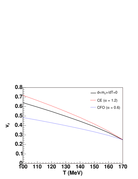
where $v_{r}(T^{\mathrm{ch}})=\tanh\rho_{0}(\beta_{0})$ is an initial condition for Eq. (42). Although the exact value of $\alpha$ needs much more involved dynamical calculation, radial flow qualitatively corresponds to the chemically frozen system for $0<\alpha<1$ and to the chemical equilibrium system for $\alpha>1$. It should be mentioned here that the temperature dependence of average radial flow can be described to some extent without solving hydrodynamic equations. Note that $\alpha$ should be taken as being a moderate value so that the total energy of the system (per unit rapidity) does not increase due to generation of radial flow.

Figure 7 shows temperature dependences of radial flow. The solid line shows the critical radial flow $v_{r}^{\mathrm{crit}}$ which results from $d\langle m_{T}\rangle/dT=0$. This is obtained by solving Eq. (42) with an initial condition $(T,v_{r})=(170,0.25)$ which is consistent with a value at RHIC energies Hirano:2002ds . The critical flow distinguishes the system of chemical equilibrium from that of chemical freezeout: $v_{r}(T)$ for CE (CFO) should be located above (below) this line since $d\langle m_{T}\rangle/dT<0$ for CE ($d\langle m_{T}\rangle/dT>0$ for CFO). Dashed line ($\alpha=1.2$) shows an example of radial flow in the analytic model CE, while dotted line ($\alpha=0.6$) shows the one in the analytic model CFO. These results look very similar to the results from real hydrodynamic simulations as shown in Fig. 5 in Ref. Hirano:2002ds .

Figure 8: Elliptic flow parameter as a function of transverse momentum within the analytic approach for pions. Thick solid line shows $v_{2}(p_{T})/v_{2}$ at chemical freezeout. Thin solid (dotted) line shows the result from the analytic model CFO ($\alpha=0.6$) at $T^{\mathrm{th}}=$100 (140) MeV. Dashed (dashed-dotted) line shows the result from the analytic model CE ($\alpha=1.2$) at $T^{\mathrm{th}}=$100 (140) MeV.

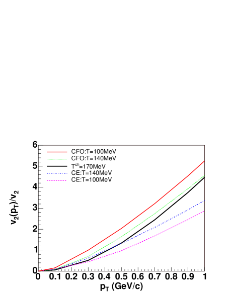
By using these profiles for radial flow, we calculate $v_{2}(p_{T})$ for pions below the chemical freezeout temperature. Hydrodynamic analysis tells us that the integrated $v_{2}$ is saturated within first 3–4 fm/$c$ just after the collision and insensitive to the late hadronic stage Kolb:2003dz . However, within our analytic approach, there is no dynamical mechanism which saturates the integrated $v_{2}$ in the late hadron stage. Therefore $v_{2}(p_{T})/v_{2}$ is the quantity to be compared with the results from full hydrodynamic simulations.

In Fig. 8, $v_{2}(p_{T})/v_{2}$ for the analytic models CE and CFO are represented. The thick solid line shows the result at $T=T^{\mathrm{ch}}=170$ MeV. The overall slope up to 1 GeV/$c$ is gradually increasing with decreasing the temperature in the analytic model CFO, while the slope is decreasing in the analytic model CE. These results clearly show that the slope of $v_{2}(p_{T})$ can vary in the late hadronic stage and that the temporal behavior of average transverse momentum $\langle p_{T}\rangle$ and radial flow $v_{r}$ is the key to understand the shape of $v_{2}(p_{T})$.

VII Conclusion and Outlook

In this paper we showed that the differential elliptic flow observable $v_{2}(p_{T})$, which is a critical component for the interpretation of RHIC data in terms of perfect fluidity of the sQGP core, is sensitive to the degree of hadro-chemical equilibrium in late time evolution of the hadronic corona. If local equilibrium hydrodynamics is applied to the hadronic corona below $T_{c}$, an inevitable logical impasse arises when confronting all the data on (1) hadron abundances (2) radial flow and (3) differential elliptic flow. In CE hydrodynamics (2) and (3) can be reproduced at the expense of (1). In PCE (1) is enforced at the expense of (2) and (3) as summarized in Table I. We presented a simple analytic blast wave model to explain these nonintuitive consequences of hadro-chemical (non)equilibrium in (P)CE implementations of hydrodynamics.

In CE both the average transverse momentum per hadron $\langle p_{T}\rangle$ and average $v_{2}$ increase with proper time in the hadronic phase in a way that accidentally preserves the slope of differential elliptic flow $dv_{2}(p_{T})/dp_{T}\approx v_{2}/\langle p_{T}\rangle$ in agreement with the data. In PCE, $\langle p_{T}\rangle$ decreases due to the basic Bjorken longitudinal cooling. The main point is that in PCE the hadronic yields are fixed at $T^{\mathrm{ch}}$ and the compensating CE “local reheating” mechanism (the conversion of heavy resonance mass back into internal energy which “mimics” a sort of dissipative effect) is absent. This is why PCE fails to describe the proton radial flow data. In addition, the slight increase of the average $v_{2}$, as in CE, with proper time cannot be compensated for in PCE. Therefore, the slope of differential elliptic flow $dv_{2}(p_{T})/dp_{T}\approx v_{2}/\langle p_{T}\rangle$ continues to grow in PCE during the hadronic phase, which leads to disagreement with RHIC data.

The subtle interplay among (1) longitudinal expansion work, (2) maintenance of hadronic abundance yields, (3) the long time development of radial flow, and (4) the differential azimuthal asymmetric elliptic flow provides a formidable dynamical constraint on the dynamics of the hadronic corona. Only by abandoning ideal hydrodynamics in the hadronic corona, have nonequilibrium hadron cascade (HC) models been able to deal with the interplay of the above hadron dynamics in a way consistent with present RHIC data. As discussed in Sec. II, this approach is natural since the viscosity to entropy ratio in a hadronic resonance gas below $T_{c}$ is too large to support even local thermal equilibrium. By relaxing both thermal and hadro-chemical equilibrium assumptions, the hybrid QGP hydrodynamics plus hadron cascade model in Teaney:2000cw has been able to account for all three major low $p_{T}$ observables as summarized in Table I. The effect of viscosity in the hadron phase Teaney:2003pb substitutes for the “local reheating” in the CE model and compensates the small growth of the average $v_{2}$ in PCE to preserve the slope of $v_{2}(p_{T})$ for pions. The slope of $v_{2}(p_{T})$ is thus found to stall at the SPS energy from the hybrid model analysis Teaney:2002aj . In the classical transport approach, both $\langle p_{T}\rangle$ Gyulassy:1997ib and $v_{2}$ Zhang:1999rs do not vary significantly when the mean free path among the particles becomes comparable with the typical gradient length scales. Moreover, the shear viscous effect changes the momentum distribution function Dumitru:2002sq and reduces the slope of $v_{2}(p_{T})$ slightly Teaney:2003pb . These are the reasons why the slope of $v_{2}(p_{T})$ does not changed significantly in the hadronic transport stage.

So how robust is the statement that hydrodynamic description at RHIC works remarkably well? We emphasized that the behavior of $v_{2}$ differs from that of $v_{2}(p_{T})$: The integrated elliptic flow does not develop so much in the late hadronic stage in which either the inviscid, chemical (non-)equilibrium fluid or the dissipative gas is assumed, whereas the differential elliptic flow depends largely on these assumptions. The large magnitude of integrated $v_{2}$ observed at RHIC is reproduced only when a small $\eta/s$ is assumed Molnar:2001ux . Therefore the large $v_{2}$ developed in the early stage is obtained from the evolution of the sQGP core, which as discussed in Sec. II must have near minimal viscosity $\eta_{\mathrm{SYM}}\approx T^{3}$. Even though the minimal sQGP viscosity is larger than the viscosity of the HRG corona, the core exhibits near perfect fluid behavior due to the deconfinement of almost all the QCD degrees of freedom. The near perfect fluidity of the sQGP core is therefore a signal of deconfinement. On the other hand, the breaking of local and hadro-chemical equilibrium in the hadronic corona is critical for this interpretation of RHIC data. If inviscid ideal hydrodynamics were valid in both sQGP and HRG phases, the crucial $v_{2}(p_{T})$ would be sensitive to the hadronic thermal freezeout dynamics and not only to the equation of state of sQGP matter.

Perhaps most surprising in connection with the hydrodynamics robustness question is the important role played by hadro-chemical freezeout at $T^{\mathrm{ch}}\approx T_{c}$ that is implied by the extensive systematics of observed hadron abundances Braun-Munzinger:2003zd . Without this constraint the different hadro-chemical results with CE and PCE would preclude a conclusion about the perfect fluidity of the sQGP core as well as the highly dissipative, imperfect fluidity of its hadronic resonance corona.

Despite the success of the hybrid HC approach, there exist open technical questions that must be still investigated. One important issue is the violation of energy-momentum conservations at the boundary between the QGP and hadron phases Bugaev:2002ch . The Cooper-Frye prescription Cooper:1974mv is employed to obtain the particle distribution just after hadronization which is to be used as an initial condition in the sequential cascade calculation. The violation is expected to be small when radial flow is large. Nevertheless there always exists in the space-like hypersurface $d\sigma^{\mu}$ in-coming particles which contributes to the number of particles negatively. This negative contribution is omitted in the actual calculations, which causes the violation of energy-momentum conservation. Proper treatment of the boundary condition may lead to change the dynamics in the QGP phase Bugaev:2002ch . In this connection, the approximate continuity of the viscosity from the sQGP to the HRG phase discussed in Sec. II minimizes this interface problem since there is no discontinuity of the stress tensor including the viscous correction at $T_{c}$.

Another important future problem is the rapidity dependence of elliptic flow. The (3+1)-dimensional ideal hydrodynamic calculations Hirano:2001eu ; Hirano:2002ds have not been able to reproduce the observed pseudorapidity dependence of $v_{2}$ in forward rapidity region at RHIC Back:2002gz . The forward rapidity region at RHIC is similar to the midrapidity region at SPS in the sense that local particle density $(1/S)dN_{\mathrm{ch}}/dy$ is similar. Heinz and Kolb Heinz:2004et proposed a “thermalization coefficient” to describe enhanced nonequilibrium effects in the low particle density region defined from the experimental data $v_{2}/\varepsilon$ as a function of $(1/S)dN_{\mathrm{ch}}/dy$ Alt:2003ab . To address correctly the rapidity and beam energy dependence taking into account the highly viscous nature of the hadronic corona, a new hybrid model must be developed in which the (3+1)-D hydrodynamic model for the sQGP core is combined with the HRG transport approach for the dissipative hadronic corona. Hirano and Nara Hirano:2004rs ; Hirano:2003pw ; Hirano:2002sc have already developed a dynamical model to describe three different aspects of relativistic heavy ion collisions in one consistent framework: Color glass condensate initial conditions for high energy colliding nuclei, hydrodynamic evolution in 3D space for long wave length components of produced matter, and quenching jets for short wave length components. A further unified framework by combining a hadronic cascade model with the above one HiranoNara will be necessary to understand more quantitatively the dynamics and the properties of QCD matter produced in relativistic heavy ion collisions at all SPS, RHIC and LHC energies.

We emphasize that continued work toward such a unified dynamical framework will be essential to further test our physical interpretation of RHIC data - as outlined in the introduction and analyzed in sections II-VI - that “perfect fluidity” of the higher viscosity sQGP core and “imperfect fluidity” of the lower viscosity HRG corona taken together with hadro-chemical equilibrium near $T_{c}\sim 160-170$ MeV already provide a compelling set of signatures for QCD deconfinement at RHIC.

Appendix A Derivation of Eq. (24)

Let us recall the formulae for modified Bessel functions

$$2K_{1}(z) = \int_{-\infty}^{\infty}dx\cosh x\exp(-z\cosh x),$$ (46)

$$2\pi I_{2}(z) = \int_{-\pi}^{\pi}d\phi\cos 2\phi\exp(z\cos\phi).$$ (47)

The numerator of Eq. (23) becomes

$$\int d\phi_{p}\cos 2\phi_{p}\int d\phi\int dy\cosh y\exp(A)$$ (48)

$$= \int d\phi 2K_{1}(B)\times 2\pi\cos 2\phi I_{2}(C),$$

where,

$$B=\frac{m_{T}\sqrt{1+u_{\perp}^{2}}}{T}+\varepsilon\frac{m_{T}u_{\perp}^{2}\cos 2\phi}{T\sqrt{1+u_{\perp}^{2}}},$$

$$C=\frac{p_{T}u_{\perp}}{T}+\varepsilon\frac{p_{T}u_{\perp}\cos 2\phi}{T}.$$

We here assume $\varepsilon$ is small, expand the modified Bessel function, and take the first order term with respect to $\varepsilon$,

$$4\pi\int d\phi\left(K_{1}+\varepsilon K_{1}^{\prime}\frac{m_{T}u_{\perp}^{2}\cos 2\phi}{T\sqrt{1+u_{\perp}^{2}}}\right)$$ (49)

$$\times \left(I_{2}+\varepsilon I_{2}^{\prime}\frac{p_{T}u_{\perp}\cos 2\phi}{T}\right)$$

$$\approx 4\pi^{2}\varepsilon\left(K_{1}^{\prime}I_{2}\frac{m_{T}u_{\perp}^{2}}{T\sqrt{1+u_{\perp}^{2}}}+K_{1}I_{2}^{\prime}\frac{p_{T}u_{\perp}}{T}\right).$$

Let us also recall some useful formulae for the derivatives of modified Bessel functions,

$$K_{n}^{\prime}(z) = -K_{n-1}(z)-\frac{n}{z}K_{n}(z),$$ (50)

$$I_{n}^{\prime}(z) = \frac{1}{2}\left[I_{n-1}(z)+I_{n+1}(z)\right].$$ (51)

Then the numerator of Eq. (23) is proportional to

$$4\pi^{2}\varepsilon \left[-\left(K_{0}+\frac{K_{1}}{z}\right)I_{2}\frac{m_{T}u_{\perp}^{2}}{T\sqrt{1+u_{\perp}^{2}}}\right.$$ (52)

$$\left.+\frac{1}{2}\left(I_{1}+I_{3}\right)K_{1}\frac{p_{T}u_{\perp}}{T}\right].$$

Here the arguments of $K$ and $I$ are, respectively, $z_{E}=m_{T}\sqrt{1+u_{\perp}^{2}}/T$ and $z_{p}=p_{T}u_{\perp}/T$. An analogous calculation can be done for the denominator of Eq. (23). The result is proportional to $4\pi^{2}\times 2K_{1}I_{0}$.

References

- (1) K. H. Ackermann et al. [STAR Collaboration], Phys. Rev. Lett. 86, 402 (2001) [arXiv:nucl-ex/0009011]; C. Adler et al. [STAR Collaboration], Phys. Rev. Lett. 87, 182301 (2001) [arXiv:nucl-ex/0107003]; Phys. Rev. Lett. 89, 132301 (2002) [arXiv:hep-ex/0205072]; Phys. Rev. C 66, 034904 (2002) [arXiv:nucl-ex/0206001]; J. Adams et al. [STAR Collaboration], arXiv:nucl-ex/0409033.
- (2) K. Adcox et al. [PHENIX Collaboration], Phys. Rev. Lett. 89, 212301 (2002) [arXiv:nucl-ex/0204005]; S. S. Adler et al. [PHENIX Collaboration], Phys. Rev. Lett. 91, 182301 (2003) [arXiv:nucl-ex/0305013].
- (3) B. B. Back et al. [PHOBOS Collaboration], Phys. Rev. Lett. 89, 222301 (2002) [arXiv:nucl-ex/0205021]; arXiv:nucl-ex/0406021; arXiv:nucl-ex/0407012.
- (4) C. Alt et al. [NA49 Collaboration], Phys. Rev. C 68, 034903 (2003) [arXiv:nucl-ex/0303001].
- (5) G. Agakichiev et al. [CERES/NA45 Collaboration], Phys. Rev. Lett. 92, 032301 (2004) [arXiv:nucl-ex/0303014].
- (6) M. M. Aggarwal et al. [WA98 Collaboration], arXiv:nucl-ex/0410045.
- (7) P. F. Kolb, P. Huovinen, U. W. Heinz and H. Heiselberg, Phys. Lett. B 500, 232 (2001) [arXiv:hep-ph/0012137]; P. Huovinen, P. F. Kolb, U. W. Heinz, P. V. Ruuskanen and S. A. Voloshin, Phys. Lett. B 503, 58 (2001) [arXiv:hep-ph/0101136]; P. F. Kolb, U. W. Heinz, P. Huovinen, K. J. Eskola and K. Tuominen, Nucl. Phys. A 696, 197 (2001) [arXiv:hep-ph/0103234]; P. Huovinen, Nucl. Phys. A 761, 296 (2005) [arXiv:nucl-th/0505036].
- (8) T. Hirano, Phys. Rev. C 65, 011901 (2002) [arXiv:nucl-th/0108004].
-
(9)
http://www.bnl.gov/bnlweb/pubaf/pr/PR
_display.asp ?prID=05-38 - (10) T. D. Lee, Nucl. Phys. A 750 (2005) 1.
- (11) M. Gyulassy and L. McLerran, Nucl. Phys. A 750, 30 (2005) [arXiv:nucl-th/0405013].
- (12) E. V. Shuryak, Nucl. Phys. A 750, 64 (2005) [arXiv:hep-ph/0405066].
- (13) C. Iso, K. Mori, and M. Namiki, Prog. Theor. Phys. 22, 403 (1959).
- (14) H. Stoecker, Nucl. Phys. A 750, 121 (2005) [arXiv:nucl-th/0406018]; S. A. Bass, M. Gyulassy, H. Stocker and W. Greiner, J. Phys. G 25, R1 (1999) [arXiv:hep-ph/9810281].
- (15) A. Hosoya and K. Kajantie, Nucl. Phys. B 250, 666 (1985).
- (16) P. Danielewicz and M. Gyulassy, Phys. Rev. D 31, 53 (1985).
- (17) M. H. Thoma, Phys. Lett. B 269, 144 (1991).
- (18) D. Molnar and M. Gyulassy, Nucl. Phys. A 697, 495 (2002) [Erratum-ibid. A 703, 893 (2002)] [arXiv:nucl-th/0104073].
- (19) S. Gavin, Nucl. Phys. A 435, 826 (1985).
- (20) A. Muronga, Phys. Rev. C 69, 044901 (2004) [arXiv:nucl-th/0309056].
- (21) Reynolds number, namely the ratio of the kinetic term to the dissipative term, is also one of the relevant quantities to see how “perfect” a fluid behaves. However, one needs full solutions of causal, dissipative hydrodynamic equations to evaluate the Reynolds number. For recent progresses of numerical solutions of causal viscous hydrodynamic equations, see, A. Muronga, Phys. Rev. Lett. 88, 062302 (2002) [Erratum-ibid. 89, 159901 (2002)] [arXiv:nucl-th/0104064]; Phys. Rev. C 69, 034903 (2004) [arXiv:nucl-th/0309055]; A. Muronga and D. H. Rischke, arXiv:nucl-th/0407114; A. K. Chaudhuri and U. W. Heinz, arXiv:nucl-th/0504022.
- (22) J. D. Bjorken, Phys. Rev. D 27, 140 (1983).
- (23) D. Teaney, Phys. Rev. C 68, 034913 (2003).
- (24) O. Kaczmarek, F. Karsch, E. Laermann and M. Lutgemeier, Phys. Rev. D 62, 034021 (2000) [arXiv:hep-lat/9908010]; O. Kaczmarek, F. Karsch, F. Zantow and P. Petreczky, Phys. Rev. D 70, 074505 (2004) [arXiv:hep-lat/0406036].
- (25) P. Kovtun, D. T. Son and A. O. Starinets, Phys. Rev. Lett. 94, 111601 (2005) [arXiv:hep-th/0405231]; G. Policastro, D. T. Son and A. O. Starinets, Phys. Rev. Lett. 87, 081601 (2001) [arXiv:hep-th/0104066]. A. Buchel, Phys. Lett. B 609, 392 (2005) [arXiv:hep-th/0408095].
- (26) K. Schalm, private communication: Note that in the limit needed in the AdS/CFT correspondence, the SYM world has adjoint vector gluons, massless complex adjoint scalars, massless adjoint Majorana spin 1/2 fermions, and no fundamental Dirac quarks. The great simplification of this model is its conformal, non-running coupling with .
- (27) S. S. Gubser, I. R. Klebanov and A. A. Tseytlin, Nucl. Phys. B 534, 202 (1998) [arXiv:hep-th/9805156].
- (28) A. Nakamura and S. Sakai, Phys. Rev. Lett. 94, 072305 (2005) [arXiv:hep-lat/0406009].
- (29) A. Peshier and W. Cassing, Phys. Rev. Lett. 94, 172301 (2005) [arXiv:hep-ph/0502138].
- (30) E. Shuryak, Prog. Part. Nucl. Phys. 53, 273 (2004) [arXiv:hep-ph/0312227].
- (31) Z. Xu and C. Greiner, arXiv:hep-ph/0406278.
- (32) T. Hirano and Y. Nara, Nucl. Phys. A 743, 305 (2004) [arXiv:nucl-th/0404039]; J. Phys. G 31, S1 (2005) [arXiv:nucl-th/0409045]; J. Phys. G 30, S1139 (2004) [arXiv:nucl-th/0403029].
- (33) S. Muroya and N. Sasaki, Prog. Theor. Phys. 113, 457 (2005) [arXiv:nucl-th/0408055].
- (34) M. Asakawa and T. Hatsuda, Phys. Rev. Lett. 92, 012001 (2004) [arXiv:hep-lat/0308034].
- (35) S. Datta, F. Karsch, P. Petreczky and I. Wetzorke, Phys. Rev. D 69, 094507 (2004) [arXiv:hep-lat/0312037].
- (36) U. W. Heinz and P. F. Kolb, arXiv:hep-ph/0204061; M. Gyulassy and D. H. Rischke, Heavy Ion Phys. 17, 261 (2003).
- (37) C. Adler et al. [STAR Collaboration], Phys. Rev. Lett. 87, 082301 (2001) [arXiv:nucl-ex/0107008]; J. Adams et al. [STAR Collaboration], arXiv:nucl-ex/0411036.
- (38) K. Adcox et al. [PHENIX Collaboration], Phys. Rev. Lett. 88, 192302 (2002) [arXiv:nucl-ex/0201008]; S. S. Adler et al. [PHENIX Collaboration], Phys. Rev. Lett. 93, 152302 (2004) [arXiv:nucl-ex/0401003].
- (39) B. B. Back et al. [PHOBOS Collaboration], arXiv:nucl-ex/0409001.
- (40) Z. w. Lin, C. M. Ko and S. Pal, Phys. Rev. Lett. 89, 152301 (2002) [arXiv:nucl-th/0204054]; Z. W. Lin, C. M. Ko, B. A. Li, B. Zhang and S. Pal, arXiv:nucl-th/0411110.
- (41) K. Adcox et al. [PHENIX Collaboration], arXiv:nucl-ex/0410003.
- (42) U. W. Heinz, Nucl. Phys. A 638, 357C (1998) [arXiv:nucl-th/9801050].
- (43) E. V. Shuryak, Nucl. Phys. A 638, 207 (1998) [arXiv:hep-ph/9801393].
- (44) P. Braun-Munzinger, K. Redlich and J. Stachel, in Quark Gluon Plasma 3, (World Scientific Pub., 2004, eds. R.C. Hwa, X.N. Wang) p. 491 [arXiv:nucl-th/0304013].
- (45) N. Arbex, F. Grassi, Y. Hama and O. Socolowski, Phys. Rev. C 64, 064906 (2001).
- (46) T. Hirano and K. Tsuda, Phys. Rev. C 66, 054905 (2002) [arXiv:nucl-th/0205043].
- (47) D. Teaney, arXiv:nucl-th/0204023.
- (48) P. F. Kolb and R. Rapp, Phys. Rev. C 67, 044903 (2003) [arXiv:hep-ph/0210222].
- (49) H. Bebie, P. Gerber, J. L. Goity and H. Leutwyler, Nucl. Phys. B 378, 95 (1992).
- (50) S. A. Bass and A. Dumitru, Phys. Rev. C 61, 064909 (2000) [arXiv:nucl-th/0001033]; S. Soff, S. A. Bass and A. Dumitru, Phys. Rev. Lett. 86, 3981 (2001) [arXiv:nucl-th/0012085].
- (51) D. Teaney, J. Lauret and E. V. Shuryak, Phys. Rev. Lett. 86, 4783 (2001) [arXiv:nucl-th/0011058]; arXiv:nucl-th/0110037.
- (52) P. Huovinen, in Quark Gluon Plasma 3, (World Scientific Pub., 2004, eds. R.C. Hwa, X.N. Wang) p. 600 [arXiv:nucl-th/0305064].
- (53) P. F. Kolb and U. Heinz, in Quark Gluon Plasma 3, (World Scientific Pub., 2004, eds. R.C. Hwa, X.N. Wang) p. 634 [arXiv:nucl-th/0305084].
- (54) T. Hirano, Acta Phys. Polon. B 36, 187 (2005) [arXiv:nucl-th/0410017].
- (55) M. Gyulassy and T. Matsui, Phys. Rev. D 29 (1984) 419.
- (56) P. V. Ruuskanen, Phys. Lett. B 147, 465 (1984).
- (57) A. N. Makhlin and Y. M. Sinyukov, Z. Phys. C 39, 69 (1988).
- (58) T. Hirano and Y. Nara, Phys. Rev. C 69, 034908 (2004) [arXiv:nucl-th/0307015].
- (59) J. Y. Ollitrault, Phys. Rev. D 46, 229 (1992).
- (60) If is a linear function of , i.e , the equality holds exactly.
- (61) J. Adams et al. [STAR Collaboration], arXiv:nucl-ex/0501009.
- (62) S. Pratt and S. Pal, Phys. Rev. C 71, 014905 (2005) [arXiv:nucl-th/0409038].
- (63) F. Cooper and G. Frye, Phys. Rev. D 10, 186 (1974).
- (64) E. Schnedermann and U. W. Heinz, Phys. Rev. C 47, 1738 (1993).
- (65) M. Gyulassy, Y. Pang and B. Zhang, Nucl. Phys. A 626, 999 (1997) [arXiv:nucl-th/9709025].
- (66) B. Zhang, M. Gyulassy and C. M. Ko, Phys. Lett. B 455, 45 (1999) [arXiv:nucl-th/9902016].
- (67) A. Dumitru, arXiv:nucl-th/0206011.
- (68) K. A. Bugaev, Phys. Rev. Lett. 90, 252301 (2003) [arXiv:nucl-th/0210087]; Phys. Rev. C 70, 034903 (2004) [arXiv:nucl-th/0401060].
- (69) U. Heinz and P. F. Kolb, J. Phys. G 30, S1229 (2004) [arXiv:nucl-th/0403044].
- (70) T. Hirano and Y. Nara, Phys. Rev. C 66, 041901 (2002) [arXiv:hep-ph/0208029]; Phys. Rev. Lett. 91, 082301 (2003) [arXiv:nucl-th/0301042]; Phys. Rev. C 68, 064902 (2003) [arXiv:nucl-th/0307087];
- (71) T. Hirano, U. W. Heinz, D. Kharzeev, R. Lacey and Y. Nara, nucl-th/0511046.