Momentum spectra, anisotropic flow, and ideal fluids

Abstract

If the matter produced in ultrarelativistic heavy-ion collisions reaches thermal equilibrium, its subsequent evolution follows the laws of ideal fluid dynamics. We show that general predictions can be made on this basis alone, irrespective of the details of the hydrodynamical model. We derive several scaling rules for momentum spectra and anisotropic flow (in particular the elliptic flow, $v_{2}$, and the hexadecupole flow, $v_{4}$) of identified particles. Comparison with existing data is briefly discussed, and qualitative predictions are made for LHC.

An ultrarelativistic Au-Au collision at RHIC produces a dense system of interacting particles and fields, which then expands into the vacuum. Ideal-fluid models have been succesful in describing this expansion Kolb:2003dz : they are able, to a certain extent, to reproduce the magnitude and the transverse momentum ($p_{t}$) dependence of elliptic flow of identified particles, together with their $p_{t}$ spectra, for momenta $p_{t}\lesssim 2$ GeV/c.

In this Letter, we derive general properties of momentum spectra of identified particles emitted by an ideal fluid, which do not depend on the specific model used. We shall introduce an important distinction between slow particles, whose velocity equals the fluid velocity at some point, and fast particles, whose velocity exceeds the maximum fluid velocity. We discuss in detail the implications of ideal-fluid behaviour for both slow and fast particles.

The expansion of a plasma into a vacuum goes through successive steps. If the particle mean free path inside the plasma is small enough, the plasma thermalizes, leading to a collision-dominated, isentropic expansion, which is described by ideal (i.e., inviscid) fluid dynamics. On the contrary, the late stage of the expansion is collision-free. In between, a transition regime takes place. This transition regime must in principle be modelled by transport theory, which encompasses both isentropic and collision-free limits Bass:2000ib ; Teaney:2001av .

In the context of heavy-ion collisions, however, the transition regime is most often modelled by a simple Ansatz, the sudden freeze-out approximation, which is a sharp transition between the two extremes: one first defines a space-time hypersurface $\Sigma$ along the history of the ideal fluid, on which the transition is expected to take place. At each point of $\Sigma$, free-streaming particles are emitted according to thermal distributions in the rest frame of the fluid. Integrating over $\Sigma$, one obtains for a given particle the following momentum spectrum Cooper:1974mv :

$$E\frac{dN}{d^{3}{\bf p}}=C\!\int_{\Sigma}\exp\!\left(-\frac{p^{\mu}u_{\mu}(x)}{T}\right)p^{\mu}d\sigma_{\mu},$$ (1)

where $u^{\mu}(x)$ is the fluid 4-velocity at point $x$ on $\Sigma$, $C$ is a normalization constant, and we have neglected the effects of quantum statistics (in practice, the latter may only be significant for pions at low $p_{t}$). For simplicity, we also assume that the fluid temperature $T$ is everywhere the same on $\Sigma$, but the results derived in this paper do not rely on this assumption. The possibility has also been raised that particles of different types Grassi:1994nf or with different transverse momenta $p_{t}$ Tomasik:2002qt have different freeze-out temperatures.

Let us briefly discuss the validity of the Cooper-Frye Ansatz, Eq. (1). This approximation is expected to be poor when applied to observables which are sensitive to the detailed physics at freeze-out, such as HBT radii Wiedemann:1999qn . The reason is that Eq. (1) assumes an isotropic momentum distribution in the rest frame of the fluid, while non-relativistic studies have shown that freeze-out precisely occurs when the relative difference between parallel and transverse components of the kinetic temperature becomes large hamel . On the other hand, the simple freeze-out Ansatz may be a reasonable one for computing single-particle spectra, provided that collective expansion dominates over random, thermal motion. This is known as the hypersonic approximation in the context of non-relativistic gas dynamics hamel ; cercignani . In the language of heavy-ion collisions, it can be rephrased as follows: consistency of the ideal-fluid picture requires that the freeze-out temperature be much smaller than the inverse slope parameters obtained by exponential fits to transverse-mass spectra Bearden:1996dd . The best-fit value of the freeze-out temperature at RHIC is $T\sim 100$ MeV Retiere:2003kf ; Hirano:2004rs , while the inverse slope parameter for pions is $T_{\rm eff}=210$ MeV Adler:2003cb . The value of $T$ is large enough to expect significant deviations from ideal-fluid behaviour, i.e., viscous effects Teaney:2003pb . It is however interesting to study the small-$T$ limit in view of upcoming heavy-ion experiments at LHC, and also to have a better grasp on viscous effects, which are easily seen as deviations from this limit.

We therefore investigate systematically the properties of momentum spectra in the limit of small $T$. The general idea is that the integral over $\Sigma$ in Eq. (1) can then be performed by means of a saddle-point integration. In physical terms, it means that the dominant contribution comes from the points where the energy of the particle in the fluid frame, $p^{\mu}u_{\mu}$, is minimum. For a given $p^{\mu}$, $p^{\mu}u_{\mu}$ is a function of the space components of the fluid 4-velocity, ${\bf u}$ (the fourth one being related to them through $u^{0}=\sqrt{1+{\bf u}^{2}}$), which themselves depend on the point $x$ on $\Sigma$. Since $p^{\mu}u_{\mu}$ is the energy of the particle in the fluid rest frame, its absolute minimum is the particle mass $m$. This minimum is reached when the particle is at rest with respect to the fluid, i.e., when its velocity ${\bf p}/p^{0}$ equals the fluid velocity ${\bf u}/u^{0}$ (or, equivalently, if ${\bf u}={\bf p}/m$).

This absolute minimum, however, occurs only if there exists a point on $\Sigma$ where this value of the fluid velocity is reached. This leads us to a qualitative discussion of the values taken by ${\bf u}$ at freeze-out. The longitudinal fluid velocity is expected to span almost the whole range from $-1$ to $1$ in ultrarelativistic collisions, and the simple Bjorken picture $u^{z}/u^{0}=z/t$ Bjorken:1982qr shows, at least qualitatively, how it is related to space-time coordinates. The radial fluid velocity spans a more limited range. The reason is that transverse collective flow is not initially present in the system but builds up progressively. For a given fluid rapidity $y_{f}=\frac{1}{2}\ln((u^{0}+u^{z})/(u^{0}-u^{z}))$, the transverse 4-velocity, $\sqrt{u_{x}^{2}+u_{y}^{2}}$, extends up to some maximum value $u_{\rm max}$, which may depend on $y_{f}$, and on the azimuthal angle $\phi_{f}$ for non-central collisions. As shown schematically in Fig. 1, $u_{\rm max}(y_{f},\phi_{f})$ is largest at $\phi_{f}=0$, along the direction of impact parameter. This is due to larger pressure gradients in this direction Ollitrault:1992bk , which explain the large in-plane elliptic flow observed at RHIC Ackermann:2000tr . Typical values of $u_{\rm max}$ are of order 1 at RHIC ($u_{\rm max}=\sinh\rho_{0}$ in the notations of Retiere:2003kf , with the best-fit value $\rho_{0}\simeq 0.9$).

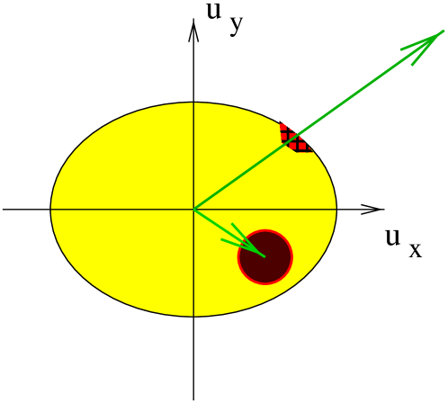
Figure 1: (Color online) Schematic representation of the distribution of the fluid transverse 4-velocity. The $x$-axis is the impact-parameter direction. The short (resp. long) arrow indicates the four-velocity of a slow (resp. fast) particle. The most probable values of the fluid four-velocity for this particle are marked as darker (red) areas.

From now on, we make a distinction between “slow” and “fast” particles as follows: a particle of mass $m$, with rapidity $y$ and transverse momentum $p_{t}$, is defined as slow if $p_{t}/m<u_{\rm max}(y,\phi)$ for all $\phi$ (that is, actually, for $\phi=\pi/2$, where the minimum occurs). Conversely, a fast particle is defined by $p_{t}/m>u_{\rm max}(y,\phi)$ for all $\phi$ (that is, for $\phi=0$, where the velocity is maximal). Between both regimes, there is a small intermediate region, which will not be considered in this Letter.

For a slow particle, there is a point on $\Sigma$ such that the fluid velocity equals the particle velocity, and the minimum $p^{\mu}u_{\mu}=m$ is reached. (Our results are unchanged if there are two or more such points.) If $T$ is small enough, the dominant contribution to the integral (1) comes from the neighbourhood of this point (see Fig. 1). The integral can then be evaluated approximately by expanding the exponent to second order around the minimum of $p^{\mu}u_{\mu}$. What remains is a Gaussian integral. For a given velocity, $p^{\mu}$ is proportional to the particle mass $m$. Hence, the width of the Gaussian varies with $m$ like $1/\sqrt{m}$, and the integral over $\Sigma$ in Eq. (1) is $m^{-3/2}$ times a function of the particle velocity. This means that the mass dependence is only a global factor for slow particles:

$$E\frac{dN}{d^{3}{\bf p}}\equiv\frac{dN}{p_{t}\,dp_{t}\,d\phi\,dy}=c(m)f\!\left(\frac{p_{t}}{m},y,\phi\right),$$ (2)

where $f$ is the same for all particles. As a result, transverse momentum and rapidity spectra (integrated over $\phi$) of identified slow particles coincide, up to a normalization factor, when they are plotted as a function of $p_{t}/m$ and $y$. The coefficients quantifying azimuthal anisotropies $v_{n}=\langle\cos n\phi\rangle$, which are independent of the total yield, should coincide for different identified slow particles at the same $p_{t}/m$ and $y$. This property holds for directed flow $v_{1}$ as well as for elliptic flow $v_{2}$ and the higher harmonics. The behaviour is qualitatively correct for $v_{2}$ at RHIC, which rises more slowly with $p_{t}$ for heavier particles Adams:2004bi ; Adler:2003kt .

The condition under which the saddle-point approximation is good for slow particles can be roughly stated as $T\ll m$ for a relativistic fluid, for dimensional reasons: the larger $m$, the smaller the width of the Gaussian, and the better the approximation. A detailed calculation gives the condition

$$T\ll mv_{\rm max}^{2}$$ (3)

with $v_{\rm max}\equiv u_{\rm max}/u^{0}_{\rm max}$ and $u^{0}_{\rm max}=\sqrt{1+u_{\rm max}^{2}}$; this condition amounts to assuming that collective motion dominates over thermal motion. At RHIC, we expect the approximation to be poor for pions (furthermore, the pion spectrum is contaminated at low $p_{t}$ by secondary decays, and may also be sensitive to Bose–Einstein statistics), but it might be a reasonable one for kaons and heavier hadrons with $p_{t}<m$/c.

Let us now discuss fast particles. Roughly speaking, these are the particles that move faster than the fluid: the minimum value of $p^{\mu}u_{\mu}$ is larger than $m$. In order to locate this minimum, we denote by $y$ (resp. $y_{f}$) the particle (resp. fluid) longitudinal rapidity, by $u_{\parallel}$ the transverse component of ${\bf u}$ parallel to the particle transverse momentum ${\bf p}_{t}$, and by $u_{\perp}$ the transverse component of ${\bf u}$ orthogonal to ${\bf p}_{t}$. With these notations,

$$p^{\mu}u_{\mu}=m_{t}\cosh(y-y_{f})\sqrt{1+u_{\parallel}^{2}+u_{\perp}^{2}}-p_{t}u_{\parallel},$$ (4)

where $m_{t}\equiv\sqrt{m^{2}+p_{t}^{2}}$. Minimization with respect to $y_{f}$ and $u_{\perp}$ gives $y_{f}=y$ and $u_{\perp}=0$, i.e., the fluid velocity is parallel to the particle velocity. The minimum is then attained when $u_{\parallel}$ is maximum, i.e, when $u_{\parallel}=u_{\rm max}(y,\phi)$, where $\phi$ is the azimuthal angle of the particle. In other words, fast particles come from regions on $\Sigma$ where the parallel velocity is close to its maximum value (see Fig. 1). A saddle-point integration then gives 

$$\frac{dN}{dy\,d^{2}{\bf p}_{t}}\propto\frac{1}{\sqrt{p_{t}-m_{t}v_{\rm max}}}\exp\!\left(\frac{p_{t}u_{\rm max}-m_{t}u^{0}_{\rm max}}{T}\right),$$ (5)

where the $(y,\phi)$ dependence is implicit. This result was already obtained long ago for massless particles in Ref. Blaizot:1986bh (see also Schnedermann:1993ws ).

The saddle-point approximation is valid for fast particles if $p_{t}$ is large enough. A more precise criterion is

$$T\ll\frac{(p_{t}u^{0}_{\rm max}-m_{t}u_{\rm max})^{2}}{m_{t}u^{0}_{\rm max}-p_{t}u_{\rm max}},$$ (6)

together with the condition $p_{t}>mu_{\rm max}$. At RHIC, the left-hand side (lhs) of Eq. (6) is smaller than the right-hand side (rhs) by at least a factor of 2 as soon as $p_{t}>0.7$ GeV/c for pions, $p_{t}>1.2$ GeV/c for kaons, and $p_{t}>1.8$ GeV/c for (anti)protons. On the other hand, ideal fluid dynamics is expected to break down if $p_{t}$ is too high, since high $p_{t}$ particles have been shown to be more sensitive to off-equilibrium (viscosity) effects Teaney:2003pb . Deviations from fluid-like behaviour are best seen on elliptic flow, for mesons above 1.5 GeV/c, and for baryons above 2.5 GeV/c. The window in which our approximation works is likely to be narrow, which reflects the importance of viscous effects at RHIC. Better agreement should be reached at LHC.

The $p_{t}$ spectra of identified particles are directly obtained from Eq. (5), neglecting the $\phi$ dependence of $u_{\max}$. Radial flow results in flatter $m_{t}$-spectra for heavier particles. In addition, Eq. (5) implies a breakdown of $m_{t}$-scaling: the slope of the spectrum decreases with increasing $m_{t}$ for pions, and increases for protons, in qualitative agreement with experimental findings Adler:2003cb .

For non-central collisions, we can also obtain the anisotropic flow coefficients. We expand $u_{\rm max}(\phi)$ in Fourier series, and neglect odd harmonics:

$$u_{\rm max}(\phi)=u_{\rm max}(1+2V_{2}\cos(2\phi)+2V_{4}\cos(4\phi)+\cdots).$$ (7)

The parameter $V_{2}$ is of the order of 4 % for semi-central Au-Au collisions at RHIC. It is related to the parameter $\rho_{2}$ of blast wave parameterizations Huovinen:2001cy ; Retiere:2003kf by $V_{2}=\rho_{2}/(2v_{\rm max})$. The $\phi$ distribution is obtained by inserting Eq. (7) into (5). If $T$ is small enough, the $\phi$ dependence in Eq. (5) is dominated by the exponential. Expanding the latter to first order in $V_{2}$, one obtains

$$v_{2}(p_{t})=\frac{V_{2}u_{\rm max}}{T}\left(p_{t}-m_{t}v_{\rm max}\right).$$ (8)

A similar equation was already obtained in Ref. Huovinen:2001cy in the framework of a simplified fluid model, and was shown to fit RHIC data rather well. In particular, Eq. (8) shows that the “mass ordering” which follows from Eq. (2) for slow particles persists at high $p_{t}$ in hydro: at a given $p_{t}$, heavier particles have smaller $v_{2}$.

We finally make predictions for the hexadecupole flow, $v_{4}$. We expand the exponential of Eq. (5) and look for terms in $\cos(4\phi)$. To leading order one obtains two terms:

$$v_{4}(p_{t}) \!=\! \frac{(V_{2}u_{\rm max})^{2}}{2T^{2}}\left(p_{t}-m_{t}v_{\rm max}\right)^{2}$$ (10)

$$+\,\frac{V_{4}u_{\rm max}}{T}\left(p_{t}-m_{t}v_{\rm max}\right).$$

For large enough $p_{t}$, the first term dominates over the second, which gives the simple, universal relation

$$v_{4}(p_{t})=\frac{v_{2}(p_{t})^{2}}{2}.$$ (11)

Let us derive the domain of validity of this approximation. If $u_{\rm max}(\phi)$ is a smooth function of $\phi$, one generally expects $V_{4}$ to be of order $(V_{2})^{2}$. The condition for Eq. (11) is then

$$T\ll u_{\rm max}\left(p_{t}-m_{t}v_{\rm max}\right).$$ (12)

At RHIC, the lhs is smaller than the rhs by at least a factor of 2 for pions with $p_{t}>0.8$ GeV/c. For heavier particles, Eq. (6) supersedes Eq. (12).

Our result, Eq. (10), is in contradiction with the statement that $v_{4}$ is a sensitive probe of initial conditions Kolb:2003zi : on the contrary, we find a universal result, which can be directly used as a probe of ideal fluid behaviour, not of initial conditions. The experimental value found by the STAR Collaboration Adams:2003zg is a factor of 2 to 3 higher than our prediction. Deviations from ideal-fluid behaviour are generally expected to yield higher values of $v_{4}$ Bhalerao:2005mm .

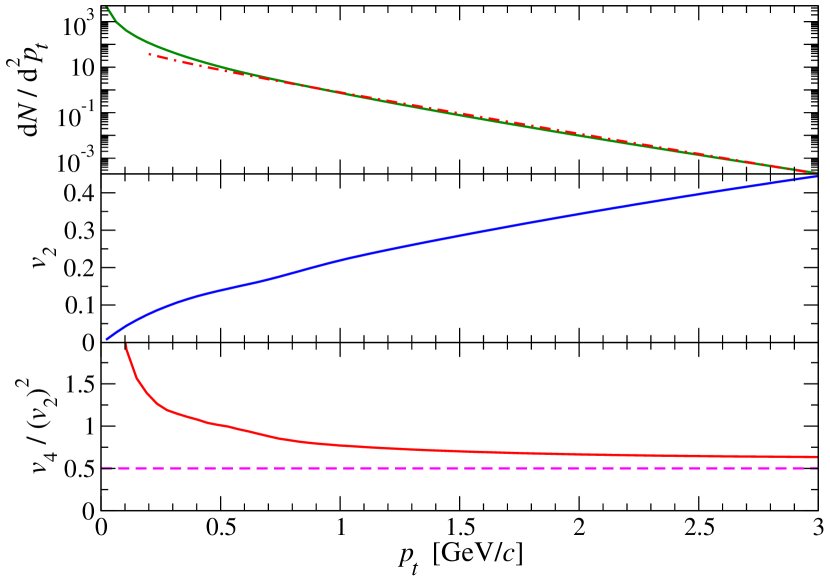
Figure 2: (color online) Numerical results from ideal hydrodynamics with Bjorken longitudinal expansion Bjorken:1982qr . and a black-body equation of state. Initial conditions mimic a midcentral ($b$=8 fm) Au-Au collision at RHIC. The initial density has been fixed to reproduce $\langle p_{t}\rangle=450$ MeV/c, as measured for pions at RHIC Adler:2003cb . Top: Solid line: $dN/dyd^{2}p_{t}$; dash-dotted line, fit using Eq. (5). Middle: $v_{2}(p_{t})$. Bottom: $v_{4}(p_{t})/v_{2}(p_{t})^{2}$.

Our results for fast particles, Eqs. (5), (8), (11), are compared to results from a numerical 3-d hydrodynamical calculation in Fig. 2. The calculation has been pushed to very large times, so that the small-$T$ limit applies. The value of $v_{4}/v_{2}^{2}$ does not go exactly to 0.5 at large $p_{t}$ but rather to 0.63. This is due to the fact that the initial eccentricity is large for this value of the impact parameter, and Eq. (11) is obtained through a leading order expansion in the anisotropy. We have checked numerically that agreement is better for lower values of $b$, where the eccentricity is smaller.

Before we come to our conclusions, let us compare our approach with the popular blast-wave one. The blast-wave parameterization, in its simplest form, assumes a unique radial velocity for the fluid Siemens:1978pb ; this framework has recently been refined to take into account the azimuthal dependence of the fluid velocity Huovinen:2001cy and of the freeze-out surface Adler:2001nb in non-central collisions, and even a distribution of fluid velocities Retiere:2003kf . A few parameters (typically four) are then fitted to experimental data. Some of the results we derived above were already obtained within the blast-wave approach, namely the mass-ordering of the $v_{2}(p_{t})$ of different types. However, our present framework is more general in the sense that we do not assume a given fluid-velocity profile, but also more specific in the sense that we assume that collective motion dominates over thermal (random) motion. In addition, blast-wave fits treat slow and fast particles on an equal footing, ignoring the distinction between both types of particles. Although fitting the whole spectrum with a single formula is admittedly more convenient, it misses an important feature of the underlying physics, since slow and fast particles originate from different regions of the expanding fluid. In particular, fits using our formulas for fast particles may yield values of $T$ and $u_{\rm max}$ which differ from blast-wave fits. Finally, our formulas are significantly simpler than blast-wave parameterizations, which involve special functions.

We have obtained the following results for momentum spectra and anisotropies in the framework of ideal-fluid models using a saddle-point approximation of the momentum distribution:

• At low $p_{t}$, identified particles of different masses have the same momentum spectra and anisotropies (up to a normalization for the spectra), when plotted as a function of velocity variables $y$ and $p_{t}/m$. This defines “slow” particles. This scaling is due to the fact that slow particles move with the fluid: they come from the regions where the fluid velocity equals their velocity. The scaling is expected to be poor for pions. It is expected to break down when $p_{t}/m$ exceeds $u_{\rm max}$, the maximum value of the transverse 4-velocity of the fluid. $u_{\rm max}$ may in general depend on the rapidity $y$, and reflects the underlying equation of state of the expanding matter.

• Fast particles, defined by Eq. (6), all originate from the region where the fluid is fastest along the direction of the particle velocity. As a result, their transverse momentum spectra and azimuthal anisotropies at a given rapidity are uniquely determined by three parameters $u_{\rm max}$, $T$, and $V_{2}$, and given by Eqs. (5), (8), (11). Comparing the $v_{2}$ of different particles should directly give the precise value of $u_{\rm max}$, while transverse momentum spectra yield $T$.

These results can be used as signatures of hydrodynamic evolution in heavy-ion collisions, and also as consistency checks of numerical ideal-fluid calculations. Ideal-fluid evolution leads to different behaviours for slow and fast particles. Some of the results obtained for fast particles (in particular for elliptic flow) are already known from blast-wave approaches. We have shown that they are in fact more general. The scaling rules for slow particles, which are evidenced here for the first time, should be further tested on available RHIC data. We expect all our results to be in closer agreement with data at LHC than at RHIC. In particular, we predict that the value of the ratio $v_{4}/(v_{2})^{2}$ should be lower at LHC than at RHIC.

References

- (1) For a recent review, see P. F. Kolb and U. Heinz, “Hydrodynamic description of ultrarelativistic heavy-ion collisions,” in Quark Gluon Plasma 3, Editors: R.C. Hwa and X.N. Wang, World Scientific, Singapore, 2004.
- (2) S. A. Bass and A. Dumitru, Phys. Rev. C 61, 064909 (2000).
- (3) D. Teaney, J. Lauret and E. V. Shuryak, nucl-th/0110037.
- (4) F. Cooper and G. Frye, Phys. Rev. D 10, 186 (1974).
- (5) F. Grassi, Y. Hama and T. Kodama, Phys. Lett. B 355, 9 (1995).
- (6) B. Tomašik and U. A. Wiedemann, Phys. Rev. C 68, 034905 (2003).
- (7) U. A. Wiedemann and U. W. Heinz, Phys. Rept. 319, 145 (1999).
- (8) B. B. Hamel and D. R. Willis, Phys. Fluids 9, 829 (1966).
- (9) C. Cercignani, The Boltzmann Equation and its Applications, Applied Mathematical Sciences vol. 67, Springer Verlag, 1988, chapter 8.
- (10) I. G. Bearden et al. [NA44 Collaboration], Phys. Rev. Lett. 78, 2080 (1997).
- (11) F. Retière and M. A. Lisa, Phys. Rev. C 70, 044907 (2004).
- (12) T. Hirano and Y. Nara, Nucl. Phys. A 743, 305 (2004).
- (13) S. S. Adler et al. [PHENIX Collaboration], Phys. Rev. C 69, 034909 (2004)
- (14) D. Teaney, Phys. Rev. C 68, 034913 (2003).
- (15) A. N. Makhlin and Y. M. Sinyukov, Z. Phys. C 39, 69 (1988).
- (16) J. D. Bjorken, Phys. Rev. D 27, 140 (1983).
- (17) J.-Y. Ollitrault, Phys. Rev. D 46, 229 (1992).
- (18) K. H. Ackermann et al. [STAR Collaboration], Phys. Rev. Lett. 86, 402 (2001).
- (19) J. Adams et al. [STAR Collaboration], Phys. Rev. C 72, 014904 (2005).
- (20) S. S. Adler et al. [PHENIX Collaboration], Phys. Rev. Lett. 91, 182301 (2003).
- (21) J.-P. Blaizot and J.-Y. Ollitrault, Nucl. Phys. A 458, 745 (1986).
- (22) E. Schnedermann, J. Sollfrank and U. W. Heinz, Phys. Rev. C 48, 2462 (1993).
- (23) P. Huovinen, P. F. Kolb, U. W. Heinz, P. V. Ruuskanen and S. A. Voloshin, Phys. Lett. B 503, 58 (2001).
- (24) P. F. Kolb, Phys. Rev. C 68, 031902 (2003).
- (25) J. Adams et al. [STAR Collaboration], Phys. Rev. Lett. 92, 062301 (2004).
- (26) R. S. Bhalerao, J. P. Blaizot, N. Borghini and J. Y. Ollitrault, Phys. Lett. B 627, 49 (2005).
- (27) P. J. Siemens and J. O. Rasmussen, Phys. Rev. Lett. 42, 880 (1979).
- (28) C. Adler et al. [STAR Collaboration], Phys. Rev. Lett. 87, 182301 (2001).