Two pion mediated scalar isoscalar NN interaction in the nuclear medium

Abstract

We study the modification of the nucleon nucleon interaction in a nuclear medium in the scalar isoscalar channel, mediated by the exchange of two correlated ($\sigma$ channel) or uncorrelated pions. For this purpose we use a standard approach for the renormalization of pions in nuclei. The corrections obtained for the $NN$ interaction in the medium in this channel are of the order of 20$\%$ of the free one in average, and the consideration of short range correlations plays an important role in providing these moderate changes. Yet, the corrections are sizable enough to suggest further studies of the stability and properties of nuclear matter.

1 Introduction

The determination of the binding energy of nuclei starting from realistic $NN$ potentials is one of the subjects which has received permanent attention from the early days when the Brueckner-Bethe-Goldstone (BBG) equation introduced methods to overcome the strong repulsion of the nuclear forces at short distances.

At present, several many body techniques compete to accurately determine the binding energy of nuclear matter starting from the realistic NN potentials. One of them is the correlated basis functions (CBF) [1, 2], which follows the line of the Hypernetted Chain Approach (FHNC) [3]. Another one follows the traditional BBG approach [4], and, although costly numerically, the variational Monte Carlo method (MC) has allowed to make, in principle, exact calculations, although limited to nuclei with small or medium value of A [5]. Methods like the selfconsistent treatment of the nucleon selfenergy have also introduced new advances in the field [6, 7, 8].

The need for three body forces has also been emphasized and the present status is that it is difficult to be quantitative on the strength of these forces, and usually they are parameterized in order to adjust the precise value of the binding energy [5, 9, 10]. It has also been noted in [11, 12, 13] that short range correlations play an important role when considering these three body forces.

A common feature of these approaches is that they start from the realistic nucleon nucleon interaction, obtained from fits to NN data and deuteron data. They use hence the free NN interaction as input. One of the important ingredients of this interaction is the one pion exchange (OPE). However, from detailed studies of the pion nuclear interaction it is well known that the pion properties in the nuclear medium are sizably renormalized [14, 15, 16, 18, 17, 19, 20].

There is also the question of the intermediate range attraction, which is basic in the binding of nuclei. Models for this interaction would contain $\sigma$ exchange, uncorrelated two pion exchange and omega exchange [21]. In as much as the pion properties are changed in the medium, so should the two pion exchange be modified. Medium effects in the two-pion exchange have been investigated in early works like in Ref. [22] restricting themselves in this case to a subset of two pion exchange diagrams with no $\Delta$-isobar intermediate states, by including Pauli blocking in the intermediate nucleons.

The medium modification of the two pion exchange got a new impulse after the models of the $\pi\pi$ interaction in the medium showed large modifications [23, 24], later on softened by the introduction of chiral constraints [25, 26]. The implementation of this medium modified $\pi\pi$ interaction in the correlated two pion exchange $NN$ potential increased appreciably the $NN$ attraction in nuclear matter. This was partially reduced by the consideration of the chiral constraints in Refs. [27, 28]. In these latter references the importance of short range correlations which modify the $\pi$ nucleus selfenergy was already discussed. The further use of medium modified vector meson masses led to improvements in the nuclear matter saturation curve.

A new perspective into this problem has been made possible by studies of meson meson interaction within chiral unitary approaches [30, 31, 32, 33, 34] which allow to improve the description of the correlated two pion exchange $NN$ interaction [29], as an alternative to the conventional $\sigma$-meson exchange interaction. This picture of the $\sigma$ exchange was mandatory after extensive studies showing that the $\sigma$ is not a genuine resonance, made up of $q\bar{q}$ but just the manifestation of a pion - pion resonance state created by the interaction of the pions, what is called a dynamically generated resonance. This shows up naturally within the context of chiral unitary approaches which use the input of the chiral Lagrangians for the meson meson interaction and extends chiral perturbation theory to implement exactly unitarity in coupled channels [30, 31, 32, 33, 34]. This means the $\sigma$ exchange inside a nuclear medium will also be modified as direct consequence of the change of the pion properties.

Our aim in the present paper is to start from this new picture for the $\sigma$ exchange, use also the standard approach for the uncorrelated two pion exchange and modify these in the nuclear medium to see what changes one finds from these sources. Further improvements come from the consideration of short range correlations not only in the pion selfenergy but also in the vertex functions appearing in the model. The changes obtained are moderate, thanks to the simultaneous consideration of these nuclear short range effects in the calculation. In the absence of these, the renormalization of the $NN$ interaction is huge. Yet, even the moderate results obtained are large enough to motivate further calculations of the nuclear binding and other properties of matter.

The paper is organized as follows. In Sec. II we provide those elements of the chiral Lagrangian which are relevant for the present calculations and briefly discuss peculiarities of the finite baryon density. In Sec. III we consider the modification of the one pion exchange $NN$ force in the nuclear medium and in Sec. IV we discuss the propagation of two pions in the nuclear matter. Sec. V and VI are devoted to the in-medium two pion exchange in the scalar-isoscalar channel, both, correlated and uncorrelated. The technical details are relegated to the Appendix.

2 Effective Lagrangian

In this section we will briefly specify those elements of the effective chiral Lagrangian in the meson-baryon sector which are relevant for the subsequent calculations.

The effective chiral Lagrangian is written as the sum of a purely mesonic Lagrangian $\mathcal{L}_{{M}}$ and the baryonic Lagrangian $\mathcal{L}_{{B}}$

$$\mathcal{L}_{{eff}}=\mathcal{L}_{M}+\mathcal{L}_{B}$$ (1)

Both are organized in a derivative and quark mass expansion. The lowest order mesonic Lagrangian $\mathcal{L}_{2}$ is given by

$$\mathcal{L}_{2}=\frac{f_{\pi}^{2}}{4}\langle\partial^{\mu}U^{\dagger}\partial_{\mu}U+\chi U^{\dagger}+U\chi^{\dagger}\rangle$$ (2)

and contains the most general low-energy interactions of the pseudo-scalar meson octet. In Eq. (2) the symbol $\langle...\rangle$ indicates the trace in flavor space, the Goldstone fields are collected in a unitary matrix $U$, $f_{\pi}\simeq 93$ MeV is the pseudoscalar decay constant and the leading symmetry-breaking term $\chi$ is linear in the quark masses. For $SU(2)$ and in the isospin limit $\chi=\mbox{diag}(m_{\pi}^{2},m_{\pi}^{2})$. The lowest order baryon octet - meson octet Lagrangian reads

$$\mathcal{L}_{B}^{(1)}=\langle\bar{B}(i\gamma^{\mu}D_{\mu}-m_{B})B\rangle+\frac{D}{2}\langle\bar{B}\gamma^{\mu}\gamma_{5}\{u_{\mu},B\}\rangle+\frac{F}{2}\langle\bar{B}\gamma^{\mu}\gamma_{5}[u_{\mu},B]\rangle$$ (3)

where the brackets $[...]$ and $\{...\}$ denote commutators and anti-commutators, respectively. The covariant derivative of the $SU(3)$ baryon matrix $B$ is defined as

$$D_{\mu}B=\partial_{\mu}B+[\Gamma_{\mu},B]$$ (4)

In the absence of external field Eqs. (3) and (4) involve other quantities

$$u=\sqrt{U},~{}~{}~{}u^{\mu}=iu^{\dagger}\nabla^{\mu}Uu^{\dagger},~{}~{}~{}\Gamma_{\mu}=\frac{1}{2}(u^{\dagger}\partial_{\mu}u+u\partial_{\mu}u^{\dagger})$$ (5)

The $SU(3)$ axial vector coupling constants are determined by neutron and hyperon $\beta$-decay. One finds $F\simeq 0.51$, $D\simeq 0.76$ and the axial coupling constant is $g_{A}=F+D\simeq 1.27$. In the $SU(2)$ limit the Lagrangian simplifies to

$$\mathcal{L}_{N}^{(1)}=\bar{\psi}(i\gamma^{\mu}D_{\mu}-m_{N})\psi+\frac{D+F}{2}\bar{\psi}\gamma^{\mu}\gamma_{5}{u}_{\mu}\psi$$ (6)

where $\psi$ is a two component Dirac field $\psi=(p,n)^{T}$.

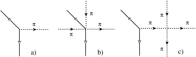
Figure 1: The $\pi NN$ vertex (a), the contact $\pi\pi\pi NN$ (b) and pion pole (c) terms.

In the pion-nucleon sector the chiral Lagrangian (6) constrains all possible interactions of the pion fields with fermions at the lowest chiral order we are working. For instance, using the exponential parameterization of the unitary matrix $U$

$$U=\exp\left[i\frac{\Phi}{f_{\pi}}\right],~{}~{}~{}~{}\Phi=\mbox{\boldmath$\tau$}\mbox{\boldmath$\pi$}$$ (7)

where $\tau$ are the Pauli operators and expanding $u$ and $u^{\dagger}$ we obtain the pion-nucleon couplings, including up to three pion fields

$$u_{\mu}=-\frac{\partial_{\mu}\Phi}{f_{\pi}}+\frac{1}{24f_{\pi}^{3}}(\partial_{\mu}\Phi\cdot\Phi^{2}-2\Phi\partial_{\mu}\Phi\cdot\Phi+\Phi^{2}\partial_{\mu}\Phi)+\mathcal{O}(\Phi^{5})$$ (8)

If we supplement Eq. (8) with the lowest order interaction of pions as provided by Eq. (2)

$$\mathcal{L}_{2}=\frac{1}{48f_{\pi}^{2}}\langle(\partial_{\mu}\Phi\cdot\Phi-\Phi\partial^{\mu}\Phi)^{2}+m^{2}_{\pi}\Phi^{4}\rangle$$ (9)

we arrive to the set of Feynman graphs shown in Fig. 1. Here, in addition to the standard $\pi NN$ vertex, Fig. 1a, the chiral perturbation theory generates the contact term of Fig. 1b (see Appendix A) and the pion pole term of Fig. 1c. These last two diagrams are the basic element in the description of $\pi N\to\pi\pi N$ reaction near the threshold [35, 36, 37, 38]. The appearance of the pole terms and contact $3\pi NN$ interactions at the same order of the chiral expansion is crucial for the in-medium calculations where due to the partial cancellations the physical amplitudes become independent of the parameterization of $U$ matrix even in the presence of the nuclear background in accord with the equivalence theorem [39]. One can see explicitely, that the contact term (b) cancels exactly the off shell part of the pion pole term (c) coming from the $(q^{2}-m_{\pi}^{2})$ part of the $\pi\pi\to\pi\pi$ vertex [40]. We shall also see that the off shell part of the $\pi\pi\to\pi\pi$ amplitude cancel exactly with other terms when we perform the calculation of the $NN$ interaction in the nuclear medium.

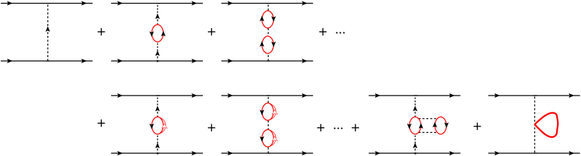
Figure 2: The OPEP diagrams. The first graph is the vacuum contribution. The second and third diagrams of the upper and first two diagrams of the lower sets of diagrams correspond to the $p-h$ and $\Delta-h$ RPA series. The last two diagrams account for the excitation of $2p-2h$ states and the contribution of the $S$-wave optical potential, respectively. The latter diagrams play a minor role and will not be further discussed.

3 One-pion exchange at finite density

We start with the one-pion exchange $NN$ potential (OPEP). The typical diagrams modifying it are shown in Fig. 2 where the propagation of exchanged pions is distorted by interactions with nucleons forming the Fermi sea. The fermionic bubbles describe the decay of the pion in $p-h$ and $\Delta-h$ states and take into account the conventional nuclear matter polarization effects. All these diagrams are responsible for the interaction of two nucleons in the particle-particle ladder channel with the in-medium virtual excitations. In Fig. 2 the first graph is the vacuum contribution. The second and third diagrams correspond to the $p-h$ RPA series and the last diagrams accounts for the excitation of $2p-2h$ states and the contribution of the $S$-wave optical potential, respectively. The $p$-wave pion self energy is given by

$$\Pi(k,\rho)=\left(\frac{D+F}{2f_{\pi}}\right)^{2}\mbox{\boldmath$k$}^{2}\mathcal{U}(k,\rho)\left[1-\left(\frac{D+F}{2f_{\pi}}\right)^{2}g^{\prime}\mathcal{U}(k,\rho)\right]^{-1}$$ (10)

where $g^{\prime}=0.6$ is the Landau-Migdal parameter [41], $\rho$ is the nuclear matter density and $\mathcal{U}(k,\rho)=\mathcal{U}^{d}(k,\rho)+\mathcal{U}^{c}(k,\rho)$ is the Lindhard function accounting for the direct and crossed contributions of $p-h$ and $\Delta-h$ excitations with the normalization of the appendix of Ref. [42].

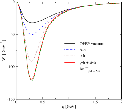
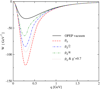
Figure 3: Left panel: The OPEP in the vacuum (solid curve) and at normal $\rho_{0}=0.16$ fm^-3 nuclear matter density (dashed curve). Right panel: OPEP at several densities.

The OPEP in the momentum space takes the form

$$-iV_{OPEP}(\mbox{\boldmath$q$},\rho) = -iW(\mbox{\boldmath$q$},\rho)\hat{\mbox{\boldmath$q$}}_{i}\hat{\mbox{\boldmath$q$}}_{j}\sigma_{1}^{i}\sigma_{2}^{j}\mbox{\boldmath$\tau$}_{1}\mbox{\boldmath$\tau$}_{2}$$ (11)

where we have defined

$$W(\mbox{\boldmath$q$},\rho)=\left(\frac{D+F}{2f_{\pi}}\right)^{2}\mbox{\boldmath$q$}^{2}F^{2}(\mbox{\boldmath$q$})\tilde{D}_{\pi}(0,\mbox{\boldmath$q$})$$ (12)

where $\tilde{D}_{\pi}(q_{0},\mbox{\boldmath$q$})$ is the pion propagator in the medium

$$i\tilde{D}_{\pi}(k)=\frac{i}{k^{2}-m^{2}_{\pi}-\Pi(k,\rho)+i0^{+}}$$ (13)

and $F(\mbox{\boldmath$q$})$ stands for a monopole form factor $\Lambda^{2}/(\Lambda^{2}+\mbox{\boldmath$q$}^{2})$ with the cut off scale $\Lambda=1$ GeV, $q$ is a momentum transfer and $\hat{\mbox{\boldmath$q$}}=\mbox{\boldmath$q$}/|\mbox{\boldmath$q$}|$. Note, that OPEP depends on the real part of the polarization operator only, since for $q=(0,\mbox{\boldmath$q$})$ one has $\mbox{Im}\Pi(0,\mbox{\boldmath$q$},\rho)=0$. The well-known vacuum $NN$ amplitude is recovered in Eq. (12) by setting $\Pi=0$ or in the limit $\rho=0$.

Our results for $W(\mbox{\boldmath$q$},\rho)$ are presented in Fig. 3 (left). The standard vacuum behavior is shown by the solid curve. The dashed curve represents the modified OPEP at normal nuclear matter density were we observe an additional strong increase of the strength associated with the attractive excitation of $p-h$ and $\Delta-h$ collective states, with $p-h$ playing a dominant role. Their individual contributions are shown by dot-dot-dashed and dot-dashed curves, respectively.

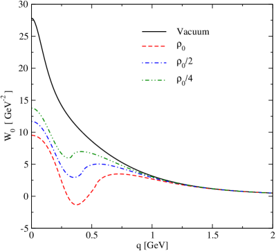
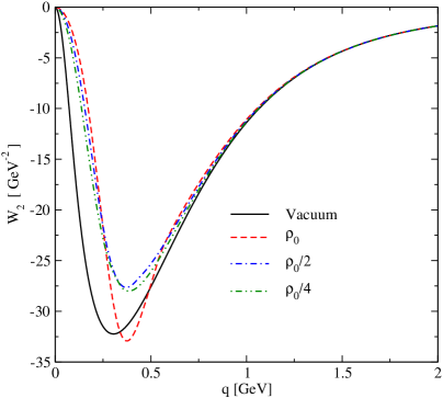
Figure 4: The OPEP with short range correlations (solid curves) as a function of the nuclear matter density. The left and right panels are the central and tensor parts, respectively.

The analytic properties of the in-medium pion propagator which we use here may be verified by using the dispersion representation for the Green function

$$i\tilde{D}_{\pi}(k_{0},\mbox{\boldmath$k$})=-i\frac{2}{\pi}\int_{0}^{\infty}dx\,x\,\frac{\mbox{Im}\tilde{D}_{\pi}(x,\mbox{\boldmath$k$})}{k_{0}^{2}-x^{2}+i0^{+}}$$ (14)

In this case the OPEP of Eq. (12) can be written in terms of the absorptive part of the pion propagator only

$$W(\mbox{\boldmath$q$},\rho)=\frac{2}{\pi}\left(\frac{D+F}{2f_{\pi}}\right)^{2}\mbox{\boldmath$q$}^{2}F^{2}(\mbox{\boldmath$q$})\int\limits_{0}^{\infty}\frac{dx}{x}\Big{[}\mbox{Im}\tilde{D}_{\pi}(x,\mbox{\boldmath$q$})\Big{]}$$ (15)

The causality requires that both equations must produce the same result. Indeed as one can see in Fig. 3 the curves calculated with dispersive and absorptive parts of the pion propagator are practically indistinguishable. We would like to note that a strong modification of the OPEP at finite baryonic density observed here is not new and was predicted long time ago by Migdal [41]. There it was also shown that in-medium modified OPEP helps to explain the unnatural parity states in finite nuclei, for instance, the shift of $0^{-}$ state in closed shell nuclei.

In the right panel of Fig. 3 we show our combined plot for a few densities $\rho_{0},\rho_{0}/2$ and $\rho_{0}/4$. Here, we also show the sensitivity of our results to the value of the Landau-Migdal parameter $g^{\prime}$. We find that the increase of $g^{\prime}$ from 0.6 to 0.7 makes the OPEP softer. This fact suggests that the proper treatment of the $NN$ short range correlations is important for understanding the in-medium properties of the OPEP.

At this point we would like to mention that in a realistic calculation one will have to add strong repulsive forces at short distances. This can be done in a straightforward way using any of many body schemes discussed in the introduction. The correlations of this part of the interaction would effectively modulate the $\pi$ exchange interaction, introducing the correlation parameter $g^{\prime}$ [43]. The denominator in Eq. (13) takes into account this effect between $p$-wave bubbles in the diagrams of Fig. 2, but not between the external nucleon and the contiguous bubble. To account for this we make the separation between the longitudinal and transverse parts of the pion effective interaction [44, 45]

$$\left(\frac{D+F}{2f_{\pi}}\right)^{2}F(\mbox{\boldmath$q$})^{2}\frac{q_{i}q_{j}}{q_{0}^{2}-\mbox{\boldmath$q$}^{2}-m_{\pi}^{2}+i0^{+}}\longrightarrow\mathcal{V}_{l}(q)\,\hat{q}_{i}\hat{q}_{j}+\mathcal{V}_{t}(q)(\delta_{ij}-\hat{q}_{i}\hat{q}_{j})$$ (16)

where $\hat{q}_{i}$ is the Cartesian component of the unit vector $\hat{\mbox{\boldmath$q$}}=\mbox{\boldmath$q$}/|\mbox{\boldmath$q$}|$ and

$$\mathcal{V}_{l}(q)=\left(\frac{D+F}{2f_{\pi}}\right)^{2}\left[\frac{\mbox{\boldmath$q$}^{2}}{q_{0}^{2}-\mbox{\boldmath$q$}^{2}-m_{\pi}^{2}+i0^{+}}+g^{\prime}\right]F(\mbox{\boldmath$q$})^{2}$$ (17)

$$\mathcal{V}_{t}(q)=\left(\frac{D+F}{2f_{\pi}}\right)^{2}\,g^{\prime}\,F(\mbox{\boldmath$q$})^{2}$$ (18)

When we perform the sum of diagrams in Fig. 2 then we get

$$V_{OPEP}(q,\rho) = \left[\frac{\mathcal{V}_{l}(q)}{1-\mathcal{U}(q,\rho)\mathcal{V}_{l}(q)}\hat{q}_{i}\hat{q}_{j}+\frac{\mathcal{V}_{t}(q)}{1-\mathcal{U}(q,\rho)\mathcal{V}_{t}(q)}(\delta_{ij}-\hat{q}_{i}\hat{q}_{j})\right]\sigma_{1}^{i}\sigma^{j}_{2}\mbox{\boldmath$\tau$}_{1}\mbox{\boldmath$\tau$}_{2}$$ (19)

$$= W_{0}(q,\rho)\mbox{\boldmath$\sigma$}_{1}\mbox{\boldmath$\sigma$}_{2}\mbox{\boldmath$\tau$}_{1}\mbox{\boldmath$\tau$}_{2}+W_{2}(q,\rho)(\mbox{\boldmath$\sigma$}_{1}\hat{\mbox{\boldmath$q$}}\mbox{\boldmath$\sigma$}_{2}\hat{\mbox{\boldmath$q$}}-\frac{1}{3}\mbox{\boldmath$\sigma$}_{1}\mbox{\boldmath$\sigma$}_{2})\mbox{\boldmath$\tau$}_{1}\mbox{\boldmath$\tau$}_{2}$$

$$W_{0}(q,\rho) = \frac{1}{3}\left[\frac{\mathcal{V}_{l}(q)}{1-\mathcal{U}(q,\rho)\mathcal{V}_{l}(q)}+\frac{2\mathcal{V}_{t}(q)}{1-\mathcal{U}(q,\rho)\mathcal{V}_{t}(q)}\right]$$ (20)

$$W_{2}(q,\rho) = \frac{\mathcal{V}_{l}(q)}{1-\mathcal{U}(q,\rho)\mathcal{V}_{l}(q)}-\frac{\mathcal{V}_{t}(q)}{1-\mathcal{U}(q,\rho)\mathcal{V}_{t}(q)}$$ (21)

where we have explicitely separated the central and the tensor parts of the interaction. In Fig. 4 we show the results for the central $W_{0}$ (left panel) and tensor $W_{2}$ (right panel) parts (omitting the spin-isospin operators) as a function of the baryonic density. Note that in the limit $\rho\to 0$, $W_{2}=W$ where $W$ is given by Eq. 12.

4 Two pions in the medium

In this section we turn to the dynamics of the two pion system in the nuclear medium. Our main interest here is the propagation of two $S$-wave pion pairs. As it is well known in the $S$-wave scattering the use of the proper unitarization schemes lead to the generation of the $\sigma$-meson. Later on we will use this result for the in-medium $NN$ interaction mediated by exchange of two correlated pions in the scalar-isoscalar $\sigma$-meson channel.

Figure 5: The unitary series representing $\pi\pi$ scattering amplitude.

For the $\pi_{a}\pi_{b}\to\pi_{c}\pi_{d}$ scattering process, defined by the Cartesian isospin indices $a,...$, the use of the standard $\chi$PT procedure in expanding the $\mathcal{L}_{2}$ of Eq. (2) to order $\mathcal{O}(\mbox{\boldmath$\pi$}^{4})$ results in the tree level contact interaction

$$-iV_{\pi\pi}^{ab\to cd}=\delta_{ab}\delta_{cd}A(s)+\delta_{ac}\delta_{bd}A(t)+\delta_{ad}\delta_{bc}A(u),$$ (22)

where

$$A(s)=\frac{i}{f_{\pi}^{2}}\Big{(}s-M_{\pi}^{2}-\frac{1}{3}\sum_{i=a,b,c,d}\Lambda_{i}\Big{)}+\mathcal{O}(q^{4}),$$ (23)

and $\Lambda_{i}=k_{i}^{2}-M_{\pi}^{2}$ is the off-shell part of the invariant $\pi\pi$ amplitude. At this order of the pion field expansion the isoscalar $S$-wave $\pi\pi$ partial amplitude ($L=0$) is obtained from the standard decomposition

$$V_{\pi\pi}^{L,I=0}=\frac{1}{2}\frac{1}{(\sqrt{2})^{\alpha}}\int_{-1}^{1}d\cos\theta~{}{P}_{L}(\cos\theta)~{}V_{\pi\pi}^{I=0}(\theta)$$ (24)

where ${P}_{L}(\cos\theta)$ are the Legendre polynomials and $(\sqrt{2})^{\alpha}$ accounts for the statistical factor occurring in states with identical particles: $\alpha=2$ for $\pi\pi\to\pi\pi$ in the unitary normalization of the states [31]. The tree level scalar-isoscalar $\pi\pi$ scattering amplitude is

$$V_{\pi\pi}^{L=I=0}=-\frac{1}{f_{\pi}^{2}}\Big{(}s-\frac{M_{\pi}^{2}}{2}-\frac{1}{3}\sum_{i}\Lambda_{i}\Big{)}.$$ (25)

In Eq. (25) the off shell part depends on choice of $U$ and is equal to zero for on mass shell pions.

Following Ref. [31] and using the Bethe-Salpeter equation we unitarize the $S$-wave $\pi\pi$ scattering amplitude (see Fig. 5)

$$V_{\pi\pi}^{L=I=0}\to{T}^{L=I=0}_{\pi\pi}=\left[{\displaystyle-{f^{2}_{\pi}}\left({s-\frac{M^{2}_{\pi}}{2}}\right)^{-1}-\displaystyle G_{\pi\pi}(s)}\right]^{-1},$$ (26)

where $G_{\pi\pi}(s)$ is a scalar two-pion loop function

$$G_{\pi\pi}(s)=i\int\frac{d^{4}k}{(2\pi)^{4}}\frac{1}{[(P-k)^{2}-M_{\pi}^{2}+i0^{+}](k^{2}-M_{\pi}^{2}+i0^{+})}$$ (27)

where $P^{\mu}=(P_{0},\mbox{\boldmath$P$})$ and $s=P^{2}$. The $G_{\pi\pi}(s)$ function is analytic with a cut along the positive real axis starting at the $\pi\pi$ threshold. Note that, Eq. (26) contains a pole in the second Riemann sheet corresponding to the $\sigma$-meson with mass and width $M-i\Gamma/2\simeq 450-i221$ MeV.

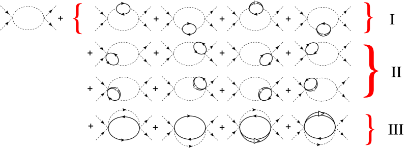
Figure 6: Renormalization of the in-medium $\pi\pi$ amplitude including $p$-hole and $\Delta$-hole excitations.

In the nuclear medium the $S$-wave $\pi\pi$ scattering amplitude and therefore the $\sigma$-meson get renormalized and explicit calculations were done in Refs. [46, 26]. The diagrams at one loop level are shown in Fig. 6. For instance, the amplitudes corresponding to the insertion of fermion bubbles in the upper meson line are given by

$$V_{\mbox{\tiny I}}^{up}(s) = i\left(\frac{D+F}{2f_{\pi}}\right)^{2}\int\frac{d^{4}k}{(2\pi)^{4}}\mbox{\boldmath$k$}^{2}\mathcal{U}(k)D^{2}_{\pi}(k)D_{\pi}(P-k)\Big{[}V_{on}(s)+\frac{1}{3f_{\pi}^{2}}\sum_{i}\Lambda_{i}\Big{]}^{2}$$ (28)

$$V_{\mbox{\tiny II}}^{up}(s) = \frac{-i2}{3f_{\pi}^{2}}\left(\frac{D+F}{2f_{\pi}}\right)^{2}\int\frac{d^{4}k}{(2\pi)^{4}}\mbox{\boldmath$k$}^{2}\mathcal{U}(k)D_{\pi}(k)D_{\pi}(P-k)\Big{[}V_{on}(s)+\frac{1}{3f_{\pi}^{2}}\sum_{i}\Lambda_{i}\Big{]}$$ (29)

$$V_{\mbox{\tiny III}}^{up}(s) = \frac{i}{9f_{\pi}^{4}}\left(\frac{D+F}{2f_{\pi}}\right)^{2}\int\frac{d^{4}k}{(2\pi)^{4}}\mbox{\boldmath$k$}^{2}\mathcal{U}(k)D_{\pi}(P-k)$$ (30)

As was shown in Refs. [46, 26], in the center of mass frame of the two pions the off shell part ($\Lambda$ terms) in $V_{I}^{up}$ cancels exactly the $V_{II}^{up}$ and $V_{III}^{up}$ terms. And one is left only with the diagrams of type (I) but with the on shell $\pi\pi$ amplitude

$$V^{up}(s) = i\left(\frac{D+F}{2f_{\pi}}\right)^{2}V_{on}^{2}(s)\int\frac{d^{4}k}{(2\pi)^{4}}\mbox{\boldmath$k$}^{2}\mathcal{U}(k)D^{2}_{\pi}(k)D_{\pi}(P-k)$$ (31)

It is straightforward to iterate the $p-h$ and $\Delta-h$ excitations in Fig. 6 (I) and the loop function, $T(s)$, is given by

$$T(s)=V_{on}^{2}(s)\cdot\tilde{G}_{\pi\pi}(s)$$ (32)

where $\tilde{G}_{\pi\pi}(s)$ is in-medium modified scalar loop integral

$$\tilde{G}_{\pi\pi}(s)=i\int\frac{d^{4}k}{(2\pi)^{4}}\tilde{D}_{\pi}(k)\tilde{D}_{\pi}(P-k)$$ (33)

Using the spectral representation for the in-medium pion propagators, Eq. (13), we get for the loop function

$$\tilde{G}_{\pi\pi}(P)=\frac{2}{\pi^{2}}\int\frac{d\mbox{\boldmath$k$}}{(2\pi)^{3}}\int\limits_{0}^{\infty}dx\Big{[}\mbox{Im}\tilde{D}_{\pi}(x,\mbox{\boldmath$k$})\Big{]}\int\limits_{x}^{\infty}dy\Big{[}\mbox{Im}\tilde{D}_{\pi}(y-x,\mbox{\boldmath$P$}-\mbox{\boldmath$k$})\Big{]}$$

$$\times\frac{y}{(P_{0}+y)(P_{0}-y+i0^{+})}$$ (34)

We refer to Ref. [47] where different aspects of $S$-wave $\pi\pi$ scattering in the nuclear medium are discussed and also the behavior of the $\sigma$-meson mass and width at finite baryonic density is addressed. But here, we would like to illustrate the impact of the nuclear medium on the $\pi\pi$ system. For that consider the imaginary part of the loop function in the $\pi\pi$ center of mass frame $P^{\mu}=(P_{0},0)$ with $P_{0}=\sqrt{s}$. This situation is relevant for the in-medium $\pi\pi$ scattering and contains the proper information about the dynamics of the pole position of $\sigma$ at finite density. Our results for the imaginary part of the scalar loop function for several densities are shown in Fig. 7(left panel). The solid curve correspond to the vacuum loop function which can be obtained from Eq. (4) by substituting the imaginary part of in-medium pion propagators by their vacuum expressions

$$\mbox{Im}\,G_{\pi\pi}(\sqrt{s})=-\frac{1}{16\pi}\sqrt{1-\frac{4m_{\pi}^{2}}{s}}$$ (35)

which is proportional to the two-body phase space of two particles (pions). As one can see in Fig. 7 (left) the effect of the medium is remarkable due to the increase of available for pions phase space because of additional pion decay branches like $p-h$, $\Delta-h$ and $2p-2h$.

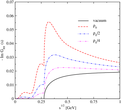
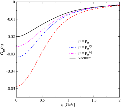
Figure 7: The imaginary part of the in-medium scalar loop function $G_{\pi\pi}$ in the $\pi\pi$ CM frame (left panel) with the normal dressing of the pion propagators including $p-h$, $\Delta-h$ and $2p-2h$ excitations. The right panel shows the loop function in the space like region $P^{\mu}=(0,\mbox{\boldmath$q$})$.

The kinematics relevant for the $NN$ force, where two nucleons interact by exchange of mesons is defined by the moving reference frame where $P^{\mu}=(0,\mbox{\boldmath$q$})$. In this case the $\pi\pi$ interaction in the medium has to be generalized from the results in [46, 26] since there $P_{0}\neq 0$ but $\mbox{\boldmath$q$}=0$. We repeat all the steps that led to cancellations in [46, 26] and find again the same cancellations as before but with some remnant $\mbox{\boldmath$q$}^{2}$ dependent terms vanishing in the limit $\mbox{\boldmath$q$}^{2}=0$. To evaluate these terms we simplify the calculation assuming $q$ relatively small (this is fine for momenta below the Fermi momentum). Concretely, we assume

$$1)~{}~{}~{}\mbox{\boldmath$q$}^{2}/k_{max}^{2}\ll 1,$$

where $k_{max}$ is the cut off in the three momentum (of the order of $1$ GeV in [31]) that one uses to regularize the $G_{\pi\pi}$ function. We also assume

$$2)~{}~{}~{}\mbox{\boldmath$k$}^{2}D_{\pi}(k)\simeq-1$$

which implies $k_{max}^{2}\gg m_{\pi}^{2}$ as it is the case. And 3) we expand $D_{\pi}(k)$ in terms of $D_{\pi}(P-k)$ and vice-versa to relate different terms. After all this is done we find that the corrections can be taken into account by means of the change in the Lindhard function

$$\mathcal{U}(k)\to\mathcal{U}(k)\left[1+\frac{\mbox{\boldmath$q$}^{2}}{3}\left(s-\displaystyle\frac{m_{\pi}^{2}}{2}\right)^{-1}+\frac{\mbox{\boldmath$q$}^{4}}{3}\left(s-\displaystyle\frac{m_{\pi}^{2}}{2}\right)^{-2}\right]$$ (36)

The expression in brackets in Eq. (36) is $\simeq 1$ for very small $q$ and also $\simeq 1$ for $\mbox{\boldmath$q$}^{2}\gg m_{\pi}^{2}/2$. Hence with very good approximation we can take the bracket equal to unity and thus there are no other corrections to be done to the result of [46, 26] except the obvious one of changing $s\to-\mbox{\boldmath$q$}^{2}$. For these value of $s$ the $G_{\pi\pi}$ is only real, contrary to the case studied in [46, 26]. Results for $G_{\pi\pi}(\mbox{\boldmath$q$}^{2})$ can be seen in Fig. 7 (right panel) for different nuclear densities $\rho_{0}$, $\rho_{0}/2$ and $\rho_{0}/4$. We can see that the corrections are sizable particularly at small values of $|\mbox{\boldmath$q$}|$.

5 In-medium renormalization of the correlated two pion ($\sigma$-meson) exchange

The correlated two pion exchange (CrTPE) in the scalar-isoscalar channel, the equivalent to a $\sigma$ exchange in meson exchange models [21], or correlated two pion exchange in the dispersion relations in [48] was studied in [29, 49] within the context of chiral Lagrangians. One starts from the diagrams of Fig. 8, where the $\pi\pi\to\pi\pi$ scattering shows the off shell ambiguities. To avoid these ambiguities with isoscalar exchange it was stated in Ref. [49] that one must include the subset of diagrams of Fig. 9 to find cancellations of the off shell $\pi\pi$ isoscalar amplitude. This statement was rigorously verified in Ref. [29], where it was shown that the consideration of these subset of chiral diagrams, Fig. 9, including the contact $3\pi NN$ interactions, results in the cancellation of the off-shell part of the $\pi\pi$ amplitude, and the on-shell part of the $\pi\pi$ amplitude can be factorized out from the loop integrals. One step forward was given in [29], where iteration of the $\pi\pi$ interaction, through the Bethe-Salpeter equation, was done by means of which a simple analytical expression was obtained for the correlated two pion exchange in the scalar-isoscalar channel

$$V_{\sigma}(t)=6V^{2}(t)\left[{\displaystyle{-f^{2}_{\pi}}\left({t-\frac{M^{2}_{\pi}}{2}}\right)^{-1}-\displaystyle G_{\pi\pi}(t)}\right]^{-1}$$ (37)

where $t=-\mbox{\boldmath$q$}^{2}$ in the $NN$ c.m. frame. The vertex function $V(t)=V_{N}(t)+V_{\Delta}(t)$ for the triangle loop with two mesons and one baryon propagator, including $N$ and $\Delta$ intermediate states, is evaluated in [29] using a cut off in $|\mbox{\boldmath$k$}|$ of about 1 GeV. Note that, the bracket in Eq. (37) contains a pole in the $s$-channel corresponding to the $\sigma$-meson. This restores the relation to the $\sigma$-meson exchange, which now enters the formalism as a dynamical resonance in the $\pi\pi$ system [29] (see also related discussions in Refs. [50, 51]).

Figure 8: Diagrams representing the correlated two pion exchange with $NN$, $N\Delta$ and $\Delta\Delta$ intermediate states.

Figure 9: The set of diagrams which cancel the off-mass shell part of the scalar-isoscalar correlated two-pion exchange.

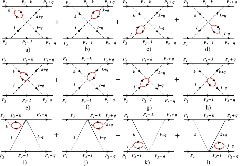
Figure 10: The in-medium diagrams involving the $p$-wave pion dressing and vertex corrections. The diagrams with the intermediate $\Delta$ states are not shown.

The diagrams responsible for the renormalization of CrTPE in the nuclear medium are shown in Fig. 10. There, in analogy to what was done for the $\pi\pi$ interaction we include $\pi$ selfenergy corrections as well as vertex corrections. We find that the cancellation of the off shell part of the vacuum $\sigma$-exchange discussed in [29] is also exact at finite baryonic density but for zero momentum transfer only (see Appendix B). The results of the derivation for $\mbox{\boldmath$q$}\neq 0$ can be summarized as follows:

1) The expressions for the triangle vertex functions $\tilde{V}_{N}$ and $\tilde{V}_{\Delta}$ of Ref. [29] are obtained in the same way replacing the two free pion propagators by the renormalized ones.

2) The Lindhard function entering the pion selfenergy is changed to

$$\mathcal{U}(k)\to\mathcal{U}(k)\cdot\left[1-\frac{1}{6}\frac{\mbox{\boldmath$q$}^{2}}{\mbox{\boldmath$q$}^{2}+\displaystyle{m_{\pi}^{2}}/{2}}\right]$$ (38)

to account for the corrections obtained at $\mbox{\boldmath$q$}\neq 0$. These corrections are negligible for small $|\mbox{\boldmath$q$}|$ and for $|\mbox{\boldmath$q$}|>m_{\pi}$ of the order of $15\%$, hence moderate in all cases.

3) The final expression for the potential $V_{\sigma}$ is given by Eq. (37), which accounts for the $\pi\pi$ rescattering, by substituting $G_{\pi\pi}(t)$ by $\tilde{G}_{\pi\pi}(t)$ of Eq. (4) and taking the expression for the in-medium vertex function $V(t)=\tilde{V}_{N}(t)+\tilde{V}_{\Delta}(t)$ where

$$\tilde{V}_{N}(t) = \frac{2\kappa_{N}}{\pi^{2}}\int\frac{d^{3}\mbox{\boldmath$k$}}{(2\pi)^{3}}\frac{M_{N}}{E(\mbox{\boldmath$k$})}\Big{(}\mbox{\boldmath$k$}^{2}+\mbox{\boldmath$k$}\mbox{\boldmath$q$}\Big{)}\int\limits_{0}^{\infty}dx\Big{[}\mbox{Im}\,\tilde{D}_{\pi}(x,\mbox{\boldmath$k$})\Big{]}$$ (39)

$$\times\int\limits_{0}^{\infty}dy\frac{x+y+E(\mbox{\boldmath$k$})-M_{N}}{(x+y)(x+E(\mbox{\boldmath$k$})-M_{N})(y+E(\mbox{\boldmath$k$})-M_{N})}\Big{[}\mbox{Im}\,\tilde{D}_{\pi}(y,\mbox{\boldmath$k$}+\mbox{\boldmath$q$})\Big{]}$$

$$\tilde{V}_{\Delta}(t) = \frac{2\kappa_{\Delta}}{\pi^{2}}\frac{4}{9}\int\frac{d^{3}\mbox{\boldmath$k$}}{(2\pi)^{3}}\frac{M_{\Delta}}{E_{\Delta}(\mbox{\boldmath$k$})}\Big{(}\mbox{\boldmath$k$}^{2}+\mbox{\boldmath$k$}\mbox{\boldmath$q$}\Big{)}\int\limits_{0}^{\infty}dx\Big{[}\mbox{Im}\,\tilde{D}_{\pi}(x,\mbox{\boldmath$k$})\Big{]}$$ (40)

$$\times\int\limits_{0}^{\infty}dy\frac{x+y+E_{\Delta}(\mbox{\boldmath$k$})-M_{N}}{(x+y)(x+E_{\Delta}(\mbox{\boldmath$k$})-M_{N})(y+E_{\Delta}(\mbox{\boldmath$k$})-M_{N})}\Big{[}\mbox{Im}\,\tilde{D}_{\pi}(y,\mbox{\boldmath$k$}+\mbox{\boldmath$q$})\Big{]}$$

The coupling constants $\kappa_{n}$ are defined by

$$\kappa_{N}=\left(\frac{D+F}{2f_{\pi}}\right)^{2},~{}~{}~{}~{}~{}\kappa_{\Delta}=\left(\frac{3}{\sqrt{2}}\frac{D+F}{2f_{\pi}}\right)^{2}$$ (41)

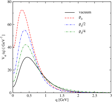
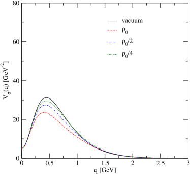
Figure 11: The momentum space unitary $\sigma$ meson exchange $NN$ potential at finite baryon density. Left panel without short range correlations. Right panel with short range correlations.

There is still one more correction to be done in order to account for short range correlations. So far we have replaced the free pion propagator by the renormalized one of Eq. (13). However, since the interaction between the $p-h$ bubble and the external nucleons is affected by correlations one should take $\mathcal{V}_{l}$ (see Eq. (17)) instead of $[(D+F)^{2}/2f_{\pi}]^{2}D_{\pi}$. Thus we would get the series

$$D_{\pi}(k)+D_{\pi}(k)\,\mathcal{U}(k)\,\mathcal{V}_{l}(k)+D_{\pi}(k)\,\mathcal{U}(k)\,\mathcal{V}_{l}(k)\,\mathcal{U}(k)\,\mathcal{V}_{l}(k)+\cdots=\frac{D_{\pi}(k)}{1-\mathcal{U}(k)\,\mathcal{V}_{l}(k)}$$

$$=\frac{\tilde{D}_{\pi}(k)}{\displaystyle 1-\left(\frac{D+F}{2f_{\pi}}\right)^{2}g^{\prime}F^{2}(k)\mathcal{U}(k)}$$ (42)

where $D_{\pi}$ and $\tilde{D}_{\pi}$ are the free and dressed pion propagators, respectively. Hence, the expressions for $\tilde{V}_{N}$ and $\tilde{V}_{\Delta}$ get modified by including inside the $\int d^{3}\mbox{\boldmath$k$}$ integral the factors

$$\frac{1}{\displaystyle 1-\left(\frac{D+F}{2f_{\pi}}\right)^{2}g^{\prime}F^{2}(k)\mathcal{U}(k)}\times\frac{1}{\displaystyle 1-\left(\frac{D+F}{2f_{\pi}}\right)^{2}g^{\prime}F^{2}(k+q)\mathcal{U}(k+q)}$$ (43)

Our results for $\sigma$-meson exchange in the momentum space are shown if Fig. 11 for both cases, no short range correlations (left) and with short range correlations (right).

6 Uncorrelated two pion exchange

In this section we consider another sort of intermediate distance contributions to the $NN$ force generated by the uncorrelated two pion exchange. The material presented here for the vacuum $NN$ scattering is standard and we merely generalize it to the nuclear medium.

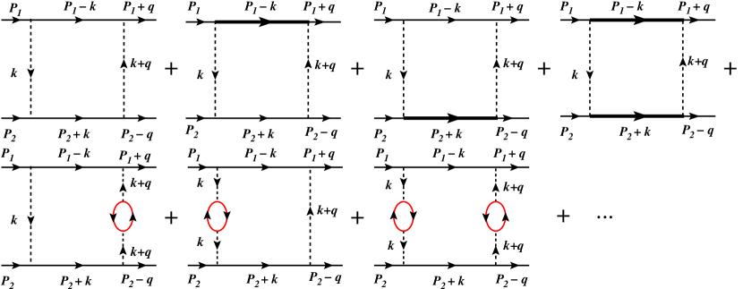
Figure 12: The planar box diagrams involving the nucleon and $\Delta$ intermediate states.

In the perturbative expansion of the $NN$ force we must to take into account the planar and crossed box diagrams shown in Figs. 12 and 13, respectively. We will discuss the scalar-isoscalar part of this contributions only. The contribution of the isovector exchange is small and can be found, for instance, in Ref. [52]

In vacuum, the expression for the planar box diagrams, Fig. 12, including the nucleon pole and $N\Delta$ and $\Delta\Delta$ intermediate states reads

$$-iV^{(P)}_{NN}=\sum_{n,m}{\kappa_{n}\kappa_{m}}\int\frac{d^{3}\mbox{\boldmath$k$}}{(2\pi)^{3}}\Big{[}\mbox{\boldmath$\Sigma$}^{(1)}_{n}\cdot(\mbox{\boldmath$k$}+\mbox{\boldmath$q$})\Big{]}\Big{[}\mbox{\boldmath$\Sigma$}^{(1)}_{n}\cdot\mbox{\boldmath$k$}\Big{]}^{\dagger}\Big{[}\mbox{\boldmath$\Sigma$}^{(2)}_{m}\cdot(\mbox{\boldmath$k$}+\mbox{\boldmath$q$})\Big{]}\Big{[}\mbox{\boldmath$\Sigma$}^{(2)}_{m}\cdot\mbox{\boldmath$k$}\Big{]}^{\dagger}\,\Big{\{}\mathcal{R}_{nm}^{(P)}(\mbox{\boldmath$k$},\mbox{\boldmath$q$})\,I_{nm}^{(P)}\Big{\}}$$ (44)

In Eq. (44) the sum over $n,m=N,\Delta$ is assumed and the spin transition operators are $\mbox{\boldmath$\Sigma$}_{N}=\mbox{\boldmath$\sigma$}$, $\mbox{\boldmath$\Sigma$}_{\Delta}=\mbox{\boldmath$S$}$. The coupling constants $\kappa_{n}$ are defined in Eq. (41). The isospin factors are given by $I_{nm}^{(P)}$ for which we find

$$I_{NN}^{(P)}=3-2\mbox{\boldmath$\tau$}_{1}\mbox{\boldmath$\tau$}_{2},~{}~{}~{}I_{N\Delta}^{(P)}=2+\frac{2}{3}\mbox{\boldmath$\tau$}_{1}\mbox{\boldmath$\tau$}_{2},~{}~{}~{}I_{\Delta\Delta}^{(P)}=\frac{4}{3}-\frac{2}{9}\mbox{\boldmath$\tau$}_{1}\mbox{\boldmath$\tau$}_{2}$$ (45)

The function $\mathcal{R}_{nm}^{(P)}$ in Eq. (44) contains the integration over the time-like component of the four vector $k$.

$$\mathcal{R}_{nm}^{(P)}(\mbox{\boldmath$k$},\mbox{\boldmath$q$}) = \int\limits_{-\infty}^{\infty}\frac{d\,k_{0}}{2\pi}D_{\pi}(k+q)\,D_{\pi}(k)\,S_{n}(P_{1}-k)\,S_{m}(P_{2}+k)$$ (46)

where $D_{\pi}$ and $S_{i}$ is the pion and nonrelativistic baryon propagators, respectively. $S_{i}$ is given by

$$iS_{i}(P)=\frac{M_{i}}{\sqrt{\mbox{\boldmath$P$}^{2}+M_{i}^{2}}}\frac{i}{P_{0}-\sqrt{\mbox{\boldmath$P$}^{2}+M_{i}^{2}}+i0^{+}}$$ (47)

This integration can be carried out explicitely

$$\mathcal{R}_{nm}^{(P)}(\omega_{1},\omega_{2}) = \frac{i}{2}\Big{[}\Big{(}\omega_{1}^{2}+\omega_{2}^{2}+3\omega_{1}\omega_{2}+[E_{n}-E][E_{m}-E]\Big{)}(E_{n}+E_{m}-2E)$$ (48)

$$+\Big{(}\omega_{1}+\omega_{2}\Big{)}\Big{(}2\omega_{1}\omega_{2}+[E_{n}+E_{m}-2E]^{2}\Big{)}\Big{]}$$

$$\times\frac{1}{\omega_{1}\omega_{2}(\omega_{1}+\omega_{2})}\left\{\frac{1}{E_{n}+E_{m}-2E-i0^{+}}\right\}$$

$$\times\frac{M_{n}}{E_{n}[\omega_{1}+E_{n}-E][\omega_{2}+E_{n}-E]}$$

$$\times\frac{M_{m}}{E_{m}[\omega_{1}+E_{m}-E][\omega_{2}+E_{m}-E]}$$

Recall that $q=(0,\mbox{\boldmath$q$})$, $P_{1}=(E,\mbox{\boldmath$P$})$, $P_{2}=(E,-\mbox{\boldmath$P$})$ in $NN$ c.m. frame and in Eq. (48)

$$\omega_{1}=\sqrt{\mbox{\boldmath$k$}^{2}+M_{\pi}^{2}},~{}~{}\omega_{2}=\sqrt{(\mbox{\boldmath$k$}+\mbox{\boldmath$q$})^{2}+M_{\pi}^{2}},~{}~{}E_{n}=\sqrt{(\mbox{\boldmath$P$}-\mbox{\boldmath$k$})^{2}+M_{n}^{2}},~{}~{}E_{m}=\sqrt{(\mbox{\boldmath$P$}-\mbox{\boldmath$k$})^{2}+M_{m}^{2}},$$ (49)

are the on-shell energies of intermediate pions and baryons with c.m. energy of the initial nucleons $E=\sqrt{\mbox{\boldmath$P$}^{2}+m}$.

In the nuclear matter $\mathcal{R}\to\tilde{\mathcal{R}}$, and the expression for $\tilde{\mathcal{R}}$ is obtained by using the dispersion representation for the in-medium pion propagator

$$\tilde{\mathcal{R}}_{nm}^{(P)}(\mbox{\boldmath$k$},\mbox{\boldmath$q$},\rho) = \frac{1}{\pi^{2}}\int\limits_{0}^{\infty}dx^{2}\int\limits_{0}^{\infty}dy^{2}\,{\mathcal{R}}_{nm}^{(P)}(x,y)\,\mbox{Im}\tilde{D}_{\pi}(x,\mbox{\boldmath$k$},\rho)\,\mbox{Im}\tilde{D}_{\pi}(y,\mbox{\boldmath$k$}+\mbox{\boldmath$q$},\rho)$$ (50)

where ${\mathcal{R}}_{nm}^{(P)}(x,y)$ is given by Eq. (48) with substitution $\omega_{1}\to x$ and $\omega_{2}\to y$.

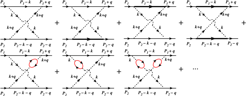
Figure 13: The crossed box diagrams with nucleon and $\Delta$ intermediate states.

For the crossed box diagrams, Fig. 13, we have

$$-iV^{(C)}_{NN}=\sum_{n,m}\kappa_{n}\kappa_{m}\int\frac{d^{3}\mbox{\boldmath$k$}}{(2\pi)^{3}}\Big{[}\mbox{\boldmath$\Sigma$}^{(1)}_{n}\cdot(\mbox{\boldmath$k$}+\mbox{\boldmath$q$})\Big{]}\Big{[}\mbox{\boldmath$\Sigma$}^{(1)}_{n}\cdot\mbox{\boldmath$k$}\Big{]}^{\dagger}\Big{[}\mbox{\boldmath$\Sigma$}^{(2)}_{m}\cdot\mbox{\boldmath$k$}\Big{]}\Big{[}\mbox{\boldmath$\Sigma$}^{(2)}_{m}\cdot(\mbox{\boldmath$k$}+\mbox{\boldmath$q$})\Big{]}^{\dagger}\,\Big{\{}\mathcal{R}_{nm}^{(C)}(\mbox{\boldmath$k$},\mbox{\boldmath$q$})\,I_{nm}^{(C)}\Big{\}}$$ (51)

The isospin factors are the following

$$I_{NN}^{(C)}=3+2\mbox{\boldmath$\tau$}_{1}\mbox{\boldmath$\tau$}_{2},~{}~{}~{}I_{N\Delta}^{(C)}=2-\frac{2}{3}\mbox{\boldmath$\tau$}_{1}\mbox{\boldmath$\tau$}_{2},~{}~{}~{}I_{\Delta\Delta}^{(C)}=\frac{4}{3}+\frac{2}{9}\mbox{\boldmath$\tau$}_{1}\mbox{\boldmath$\tau$}_{2}$$ (52)

and the vacuum expression for $\mathcal{R}_{nm}^{(C)}(\mbox{\boldmath$k$},\mbox{\boldmath$q$})$ is given by

$$\mathcal{R}_{nm}^{(C)}(\mbox{\boldmath$k$},\mbox{\boldmath$q$}) = \int\limits_{-\infty}^{\infty}\frac{d\,k_{0}}{2\pi}D_{\pi}(k+q)\,D_{\pi}(k)\,S_{n}(P_{1}-k)\,S_{m}(P_{2}-k-q)$$ (53)

The integration can be done analytically and our result reads

$$\mathcal{R}_{nm}^{(C)}(\omega_{1},\omega_{2}) = \frac{i}{2}\Big{[}\omega_{1}^{2}+\omega_{2}^{2}+\omega_{1}\omega_{2}+(\omega_{1}+\omega_{2})(\tilde{E}_{n}+E_{m}-2E)+(\tilde{E}_{n}-E)(E_{m}-E)\Big{]}$$ (54)

$$\times\frac{1}{\omega_{1}\omega_{2}(\omega_{1}+\omega_{2})}$$

$$\times\frac{M_{n}}{\tilde{E}_{n}[\omega_{1}+\tilde{E}_{n}-E][\omega_{2}+\tilde{E}_{n}-E]}$$

$$\times\frac{M_{m}}{E_{m}[\omega_{1}+E_{m}-E][\omega_{2}+E_{m}-E]}$$

here $\omega_{1},\omega_{2}$, $E$ and $E_{m}$ are defined in Eq. (49) and

$$\tilde{E}_{n}=\sqrt{(\mbox{\boldmath$P$}+\mbox{\boldmath$k$}+\mbox{\boldmath$q$})^{2}+M_{n}^{2}}$$ (55)

The corresponding expression for the in-medium crossed box diagrams takes the form

$$\tilde{\mathcal{R}}_{nm}^{(C)}(\mbox{\boldmath$k$},\mbox{\boldmath$q$},\rho)=\frac{1}{\pi^{2}}\int\limits_{0}^{\infty}dx^{2}\int\limits_{0}^{\infty}dy^{2}\,\mathcal{R}_{nm}^{(C)}(x,y)\,\mbox{Im}\tilde{D}_{\pi}(x,\mbox{\boldmath$k$},\rho)\,\mbox{Im}\tilde{D}_{\pi}(y,\mbox{\boldmath$k$}+\mbox{\boldmath$q$},\rho)$$ (56)

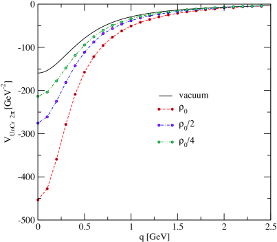
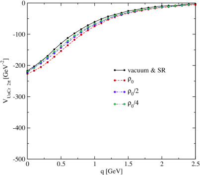
Figure 14: The momentum space uncorrelated two-pion exchange at finite baryonic density. The left panel correspond to normal pion dressing without SR correlations and right panel with SR correlations.

For the generic case of non-vanishing initial momenta the analytical structure of Eq. (48) is driven by the term in figure brackets

$$\sim\frac{1}{E_{n}+E_{m}-2E-i0^{+}}$$ (57)

Here we have to pay a special attention to the case where two intermediate $NN$ states $n=m=N$ appear, because in time ordered perturbation theory these diagrams are generated by iterations of the OPEP in a Lippmann-Schwinger equation (LSE). Considering the $NN$ intermediate state only, the iterated TPE can be easily identified and comes from the nucleon pole in Eq. (46) (in the lower half of the complex plane) corresponding to $k_{0}=E_{N}-E-i0^{+}$ with $E=\sqrt{\mbox{\boldmath$P$}^{2}+M_{N}^{2}}$

$$\mathcal{R}_{NN}^{(P)N-pole}(\omega_{1},\omega_{2})=\frac{-i}{2}\left(\frac{M_{N}}{E_{N}}\right)^{2}\frac{1}{E-E_{N}+i0^{+}}\left[\frac{1}{(E-E_{N})^{2}-\omega_{1}^{2}}\frac{1}{(E-E_{N})^{2}-\omega_{2}^{2}}\right]$$ (58)

Expanding Eq. (58) in powers of $1/M_{N}$

$$\mathcal{R}_{NN}^{(P)N-pole}(\omega_{1},\omega_{2})\simeq-i\frac{1}{\omega_{1}^{2}\omega_{2}^{2}}\frac{M_{N}}{\displaystyle\mbox{\boldmath$P$}^{2}-(\mbox{\boldmath$P$}-\mbox{\boldmath$k$})^{2}+i0^{+}}+\mathcal{O}(1/M_{N})$$ (59)

and inserting the leading order result in Eq. (44) one can get the second order term in the non-relativistic Lippmann-Schwinger equation.

It is instructive to derive the contributions of the two remaining poles (in lower half-plane) from the pion propagators

$$\mathcal{R}_{NN}^{(P)\pi-poles}(\mbox{\boldmath$k$},\mbox{\boldmath$q$})=\frac{-i}{2\omega_{1}\omega_{2}}\frac{\omega_{1}^{2}+\omega_{2}^{2}+\omega_{1}\omega_{2}-(E-E_{N})^{2}}{(\omega_{1}+\omega_{2})(\omega_{1}^{2}-(E-E_{N})^{2})(\omega_{2}^{2}-(E-E_{N})^{2})}\frac{M^{2}_{N}}{E^{2}_{N}}$$ (60)

After the expansion of this result in powers of $1/M_{N}$ we get

$$\mathcal{R}_{NN}^{(P)\pi-poles}(\mbox{\boldmath$k$},\mbox{\boldmath$q$})\simeq-\frac{i}{2}\frac{\omega_{1}^{2}+\omega_{2}^{2}+\omega_{1}\omega_{2}}{\omega_{1}^{3}\omega_{2}^{3}(\omega_{1}+\omega_{2})}+\mathcal{O}(1/M_{N})$$ (61)

In this limit Eq. (61) cancels exactly the corresponding crossed box diagram with two intermediate nucleons in the isoscalar channel. Indeed, considering the crossed box diagram with two intermediate nucleons, the leading term of $\mathcal{R}_{NN}^{(C)}(\mbox{\boldmath$k$},\mbox{\boldmath$q$})$ in the $1/M_{N}$ expansion is given by

$$\mathcal{R}_{NN}^{(C)}(\mbox{\boldmath$k$},\mbox{\boldmath$q$})\simeq\frac{i}{2}\frac{\omega_{1}^{2}+\omega_{2}^{2}+\omega_{1}\omega_{2}}{\omega_{1}^{3}\omega_{2}^{3}(\omega_{1}+\omega_{2})}+\mathcal{O}(1/M_{N})$$ (62)

Note that for the isovector $\pi\pi$ exchange because of the different sign of the $\mbox{\boldmath$\tau$}_{1}\mbox{\boldmath$\tau$}_{2}$ term in $I_{NN}^{(P)}$, $I_{NN}^{(C)}$ in Eqs. (45) and (52) these two contributions would add. The cancellation discussed above hold also in the nuclear medium.

The result of the vacuum scalar-isoscalar $NN$ force generated by the planar and crossed box diagrams, with the nucleon pole diagrams excluded, is shown in the left panel of Fig. 14 by the solid curve. It is in agreement with Ref. [52] where it was shown that the consistent use of the cut off regularization in both the correlated two pion exchange, and uncorrelated two pion exchange, together with the contribution of a repulsive $\omega$-exchange lead to a scalar-isoscalar potential in good agreement with the Argonne [53] potential in the whole range of relevant distances. The corresponding results for the nuclear matter are shown in Fig. 14 (left) for three densities $\rho_{0}$, $\rho_{0}/2$ and $\rho_{0}/4$. Qualitatively the behavior is similar to the vacuum case but with a strong enhancement toward the small momentum transfer. As we have seen this feature is generic in present calculations. Uncorrelated $\pi\pi$ exchange becomes extremely attractive at intermediate distances.

The spin sum over intermediate baryon states of the $\sim\mbox{\boldmath$\Sigma$}\cdot\mbox{\boldmath$k$}$ operator in Eqs. (44) and (51) gives in the scalar channel

$$\beta\left[(\mbox{\boldmath$k$}+\mbox{\boldmath$q$})\cdot\mbox{\boldmath$k$}\right]^{2}$$ (63)

where $\beta=1$ $(NN)$, $\beta=2/3$ $(N\Delta)$ and $\beta=4/9$ $(\Delta\Delta)$. Now we again wish to take into account the short range correlations

$$\left(\frac{D+F}{2f_{\pi}}\right)^{4}F^{2}(\mbox{\boldmath$k$})F^{2}(\mbox{\boldmath$k$}+\mbox{\boldmath$q$}){D}_{\pi}(\mbox{\boldmath$k$}+\mbox{\boldmath$q$}){D}_{\pi}(\mbox{\boldmath$k$})\left[(\mbox{\boldmath$k$}+\mbox{\boldmath$q$})\cdot\mbox{\boldmath$k$}\right]^{2}$$

$$\Longrightarrow\tilde{\mathcal{W}}_{l}(k+q)\tilde{\mathcal{W}}_{l}(k)\left[(\widehat{\mbox{\boldmath$k$}+\mbox{\boldmath$q$}})\cdot\hat{\mbox{\boldmath$k$}}\right]^{2}$$

$$+\left[\tilde{\mathcal{W}}_{l}(k+q)\tilde{\mathcal{W}}_{t}(k)+\tilde{\mathcal{W}}_{l}(k)\tilde{\mathcal{W}}_{t}(k+q)\right]\left\{1-\left[(\widehat{\mbox{\boldmath$k$}+\mbox{\boldmath$q$}})\cdot\hat{\mbox{\boldmath$k$}}\right]^{2}\right\}$$

$$+\tilde{\mathcal{W}}_{t}(k+q)\tilde{\mathcal{W}}_{t}(k)\left\{1+\left[(\widehat{\mbox{\boldmath$k$}+\mbox{\boldmath$q$}})\cdot\hat{\mbox{\boldmath$k$}}\right]^{2}\right\}$$

where

$$\tilde{\mathcal{W}}_{i}(k)=\frac{\mathcal{V}_{i}(k)}{1-\mathcal{U}(k)\mathcal{V}_{i}(k)}$$ (65)

where $\mathcal{U}(k)$ is the Lindhard function and $\mathcal{V}_{l}$ and $\mathcal{V}_{t}$ are given by Eq. (17) and  (18), respectively.

7 Results and discussions

By comparing the results in Fig. 3 and Fig. 4 we observe that the effect of correlations has been essential and reduces drastically the medium effects found in Fig. 3 without corrections. We observe that the medium corrections weaken the strength of the central part of the OPEP. On the other hand the effect of the medium corrections on the tensor part are more moderate.

The $\sigma$ exchange presents similar features as we can see in Fig. 11. There we see that the medium effects in the absence of short range correlations are rather large and increase the strength of the interaction in about a factor two at $\rho=\rho_{0}$. However, as soon as the correlations are taken into account the medium modifications are reduced drastically and at $\rho=\rho_{0}$ just reduce the strength in about 25 percent.

The medium effects in the uncorrelated two pion exchange are also relatively small, with respect to the size of the interaction in the vacuum, see Fig. 14 (right). Once again the consideration of the correlations has been essential and reducing the size of the medium effects. However, the fact that the strength of this interaction is bigger than that of the correlated two pion exchange makes the absolute correction relevant and of the same size as the corrections discussed before.

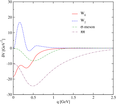
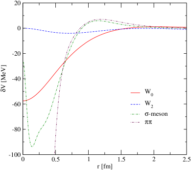
Figure 15: The modification of the $NN$ interaction at normal nuclear matter density in momentum space (left panel) and in configuration space (right panel). Shown are the central part of the OPEP (solid curve), tensor part of the OPEP (dashed curve), correlated $\sigma$-meson exchange (dot-dashed curve) and uncorrelated $\pi\pi$ exchange (dot-dot-dashed curve).

Since we have taken also the effect of correlations in the free part of the interaction and any realistic calculation of the binding energy of matter will explicitly account for these correlations, the use of our modified in-medium potentials would lead to double-counting if any of these methods is used. For this purpose the relevant results from this work should be the differences between the in-medium potential and the free one. In this case we start already with one bubble and the correlations account for the repulsion between the external leg and the one in the bubble. The two external legs still have to be correlated and this will be done with the use, for instance, of the ordinary Bethe Golstone equation.

After this discussion of the medium effects in the different terms, we show the differences in momentum space between the medium and free parts of the different terms in Fig. 15 (left). The results are shown at $\rho=\rho_{0}$ and we see that these corrections are moderate, but they could have a relevant role in the binding of matter. In order to have a qualitative idea of the relevance of these corrections to the potentials we rewrite them in coordinate space and show these results in Fig. 15 (right). The effects seem sizeable at short distances, but this will be irrelevant in any realistic calculation of binding energies since the consideration of the short range correlations between the external legs will make this interaction inoperative. More interesting is the strength of the corrections around 1 fm, and there we see that all them are relatively small, of the order of 20 MeV or less, the biggest one being the central part of the OPE. However, given the size of the empirical scalar isoscalar attraction [53] which is of the order of 20 MeV at intermediate densities, the corrections found here are not negligible. It would be thus interesting to see the effects of the results obtained here in observables like the binding of nuclear matter and other properties, which we hope to stimulate with the results obtained here.

8 Conclusions

In this paper we studied the modification of the one pion exchange, as well as two pion exchange potential inside a nuclear medium. For this purpose we separated the two pion exchange into an uncorrelated two pion exchange and the correlated two pion exchange. We study both in the scalar isoscalar channel, which is by large the most important one generated by this interaction. The correlated two pion exchange gave rise to the equivalent of the $\sigma$ exchange in other models and we studied the medium modification to it. On the other hand, for the uncorrelated two pion exchange we have followed a traditional approach in which only terms with at least one intermediate $\Delta$ state are considered.

One of the important findings here was the effect played by the NN short range correlations which drastically moderated the medium corrections to the potential. In the absence of these, the corrections where unrealistically large. Yet, even if relatively moderate, the medium corrections found in this paper are sizeable enough to have relevant repercussions in the binding and other properties of nuclear matter and we would like to encourage calculations in this direction.

Appendix A Feynman rules for vertices

The set of Feynman diagrams shown in Fig. 16 appear in the construction of the $\pi N\to\pi\pi N$ transition amplitude. The corresponding $3\pi NN$ vertex functions are given by

Figure 16: Contact terms appearing in the construction of the $\pi N\to\pi\pi N$ transition amplitude.

$$iL_{a} = \frac{D+F}{2}\frac{2\sqrt{2}}{12f_{\pi}^{3}}\Big{[}\mbox{\boldmath$\sigma$}(\mbox{\boldmath$q$}_{1}+2\mbox{\boldmath$k$}_{1}-\mbox{\boldmath$k$}_{2})\Big{]}$$ (66)

$$iL_{b} = \frac{D+F}{2}\frac{2\sqrt{2}}{12f_{\pi}^{3}}\Big{[}\mbox{\boldmath$\sigma$}(\mbox{\boldmath$q$}_{2}+2\mbox{\boldmath$k$}_{2}-\mbox{\boldmath$k$}_{1})\Big{]}$$ (67)

$$iL_{c} = \pm\frac{D+F}{2}\frac{2}{12f_{\pi}^{3}}\Big{[}\mbox{\boldmath$\sigma$}(2\mbox{\boldmath$q$}_{1}+\mbox{\boldmath$k$}_{1}+\mbox{\boldmath$k$}_{2})\Big{]}$$ (68)

$$iL_{d} = \frac{D+F}{2}\frac{2\sqrt{2}}{12f_{\pi}^{3}}\Big{[}\mbox{\boldmath$\sigma$}(2\mbox{\boldmath$q$}_{1}+\mbox{\boldmath$k$}_{1}+\mbox{\boldmath$k$}_{2})\Big{]}$$ (69)

$$iL_{e} = \frac{D+F}{2}\frac{2\sqrt{2}}{12f_{\pi}^{3}}\Big{[}\mbox{\boldmath$\sigma$}(2\mbox{\boldmath$q$}_{2}+\mbox{\boldmath$k$}_{1}+\mbox{\boldmath$k$}_{2})\Big{]}$$ (70)

$$iL_{f} = 0$$ (71)

Appendix B Correlated exchange in the medium

In this Appendix we demonstrate the cancellation of the off shell part of the correlated two pion exchange in the scalar isoscalar channel. For simplicity we consider the nucleon intermediate states only. The generalization to $N\Delta$ and $\Delta\Delta$ is straightforward. The diagrams are shown in Fig. 10 and corresponding amplitudes are given by

$$T_{a} = T_{a}^{on}+T_{a}^{(1)}+T_{a}^{(2)}$$ (72)

$$-iT_{a}^{on} = 6\left(\frac{D+F}{2f_{\pi}}\right)^{4}V^{on}_{\pi}(t)\Big{[}V_{N\pi\pi}(t)\Big{]}$$ (73)

$$\times\int\frac{d^{4}k}{(2\pi)^{4}}\Big{[}\mbox{\boldmath$\sigma$}(\mbox{\boldmath$k$}+\mbox{\boldmath$q$})\Big{]}\Big{[}\mbox{\boldmath$\sigma$}\mbox{\boldmath$k$}\Big{]}\Big{[}\mbox{\boldmath$k$}^{2}\mathcal{U}(k)\Big{]}S_{F}(P_{1}-k)D^{2}(k)D(k+q)$$

$$-iT_{a}^{(1)} = 2\left(\frac{D+F}{2f_{\pi}}\right)^{4}\frac{1}{f_{\pi}^{2}}\Big{[}V_{N\pi\pi}(t)\Big{]}$$ (74)

$$\times\int\frac{d^{4}k}{(2\pi)^{4}}\Big{[}\mbox{\boldmath$\sigma$}(\mbox{\boldmath$k$}+\mbox{\boldmath$q$})\Big{]}\Big{[}\mbox{\boldmath$\sigma$}\mbox{\boldmath$k$}\Big{]}\Big{[}\mbox{\boldmath$k$}^{2}\mathcal{U}(k)\Big{]}S_{F}(P_{1}-k)D(k)D(k+q)$$

$$-iT_{a}^{(2)} = 2\left(\frac{D+F}{2f_{\pi}}\right)^{4}\frac{1}{f_{\pi}^{2}}\Big{[}V_{N\pi\pi}(t)\Big{]}$$ (75)

$$\times\int\frac{d^{4}k}{(2\pi)^{4}}\Big{[}\mbox{\boldmath$\sigma$}(\mbox{\boldmath$k$}+\mbox{\boldmath$q$})\Big{]}\Big{[}\mbox{\boldmath$\sigma$}\mbox{\boldmath$k$}\Big{]}\Big{[}\mbox{\boldmath$k$}^{2}\mathcal{U}(k)\Big{]}S_{F}(P_{1}-k)D^{2}(k)$$

$$T_{b} = T_{b}^{on}+T_{b}^{(1)}+T_{b}^{(2)}$$ (76)

$$-iT_{b}^{on} = 6\left(\frac{D+F}{2f_{\pi}}\right)^{4}V_{\pi}^{on}(t)\Big{[}V_{N\pi\pi}(t)\Big{]}$$ (77)

$$\times\int\frac{d^{4}k}{(2\pi)^{4}}\Big{[}\mbox{\boldmath$\sigma$}(\mbox{\boldmath$k$}+\mbox{\boldmath$q$})\Big{]}\Big{[}\mbox{\boldmath$\sigma$}\mbox{\boldmath$k$}\Big{]}\Big{[}(\mbox{\boldmath$k$}+\mbox{\boldmath$q$})^{2}\mathcal{U}(k+q)\Big{]}S_{F}(P_{1}-k)D(k)D^{2}(k+q)$$

$$-iT_{b}^{(1)} = 2\left(\frac{D+F}{2f_{\pi}}\right)^{4}\frac{1}{f_{\pi}^{2}}\Big{[}V_{N\pi\pi}(t)\Big{]}$$ (78)

$$\times\int\frac{d^{4}k}{(2\pi)^{4}}\Big{[}\mbox{\boldmath$\sigma$}(\mbox{\boldmath$k$}+\mbox{\boldmath$q$})\Big{]}\Big{[}\mbox{\boldmath$\sigma$}\mbox{\boldmath$k$}\Big{]}\Big{[}(\mbox{\boldmath$k$}+\mbox{\boldmath$q$})^{2}\mathcal{U}(k+q)\Big{]}S_{F}(P_{1}-k)D(k)D(k+q)$$

$$-iT_{b}^{(2)} = 2\left(\frac{D+F}{2f_{\pi}}\right)^{4}\frac{1}{f_{\pi}^{2}}\Big{[}V_{N\pi\pi}(t)\Big{]}$$

$$\times\int\frac{d^{4}k}{(2\pi)^{4}}\Big{[}\mbox{\boldmath$\sigma$}(\mbox{\boldmath$k$}+\mbox{\boldmath$q$})\Big{]}\Big{[}\mbox{\boldmath$\sigma$}\mbox{\boldmath$k$}\Big{]}\Big{[}(\mbox{\boldmath$k$}+\mbox{\boldmath$q$})^{2}\mathcal{U}(k+q)\Big{]}S_{F}(P_{1}-k)D^{2}(k+q)$$

$$-iT_{c} = -iT_{a}(k\to l,q\to-q,P_{1}\to P_{2})$$

$$-iT_{d} = -iT_{b}(k\to l,q\to-q,P_{1}\to P_{2})$$ (79)

where $V_{N\pi\pi}(t)$ is the triangle loop integral

$$V_{N\pi\pi}(t)=i\left(\frac{D+F}{2f_{\pi}}\right)^{2}\int\frac{d^{4}l}{(2\pi)^{4}}\Big{[}\mbox{\boldmath$\sigma$}(\mbox{\boldmath$l$}-\mbox{\boldmath$q$})\Big{]}\Big{[}\mbox{\boldmath$\sigma$}\mbox{\boldmath$l$}\Big{]}S_{F}(P_{2}-l)D(l-q)D(l)$$ (80)

and the on-mass-shell $\pi\pi$ scattering amplitude is

$$V^{on}_{\pi}(t)=-\frac{1}{f_{\pi}^{2}}\Big{(}\displaystyle t-\frac{M_{\pi}^{2}}{2}\Big{)}$$ (81)

$$-iT_{e} = -\left(\frac{D+F}{2f_{\pi}}\right)^{4}\frac{1}{f_{\pi}^{2}}\Big{[}V_{N\pi\pi}(t)\Big{]}$$ (82)

$$\times\int\frac{d^{4}k}{(2\pi)^{4}}\Big{[}\mbox{\boldmath$\sigma$}(\mbox{\boldmath$k$}+\mbox{\boldmath$q$})\Big{]}\Big{[}\mbox{\boldmath$\sigma$}\mbox{\boldmath$k$}\Big{]}\Big{[}(3\mbox{\boldmath$k$}\mbox{\boldmath$q$}+2\mbox{\boldmath$k$}^{2})\mathcal{U}(k)\Big{]}S_{F}(P_{1}-k)D(k)D(k+q)$$

$$-iT_{f} = \left(\frac{D+F}{2f_{\pi}}\right)^{4}\frac{1}{f_{\pi}^{2}}\Big{[}V_{N\pi\pi}(t)\Big{]}$$

$$\times\int\frac{d^{4}k}{(2\pi)^{4}}\Big{[}\mbox{\boldmath$\sigma$}(\mbox{\boldmath$k$}+\mbox{\boldmath$q$})\Big{]}\Big{[}\mbox{\boldmath$\sigma$}\mbox{\boldmath$k$}\Big{]}\Big{[}(\mbox{\boldmath$q$}^{2}-2\mbox{\boldmath$k$}^{2}-\mbox{\boldmath$k$}\mbox{\boldmath$q$})\mathcal{U}(k+q)\Big{]}S_{F}(P_{1}-k)D(k)D(k+q)$$

$$-iT_{g} = -iT_{e}(k\to l,q\to-q,P_{1}\to P_{2})$$ (84)

$$-iT_{h} = -iT_{f}(k\to l,q\to-q,P_{1}\to P_{2})$$ (85)

$$-iT_{i} = \left(\frac{D+F}{2f_{\pi}}\right)^{4}\frac{1}{f_{\pi}^{2}}\Big{[}V_{N\pi\pi}(t)\Big{]}\int\frac{d^{4}k}{(2\pi)^{4}}\Big{[}\mbox{\boldmath$\sigma$}(\mbox{\boldmath$q$}-2\mbox{\boldmath$k$})\Big{]}\Big{[}\mbox{\boldmath$\sigma$}\mbox{\boldmath$k$}\Big{]}\Big{[}\mbox{\boldmath$k$}^{2}\mathcal{U}(k)\Big{]}S_{F}(P_{1}-k)D^{2}(k)$$ (86)

$$-iT_{j} = -\left(\frac{D+F}{2f_{\pi}}\right)^{4}\frac{1}{f_{\pi}^{2}}\Big{[}V_{N\pi\pi}(t)\Big{]}$$ (87)

$$\times\int\frac{d^{4}k}{(2\pi)^{4}}\Big{[}\mbox{\boldmath$\sigma$}\mbox{\boldmath$k$}\Big{]}\Big{[}\mbox{\boldmath$\sigma$}(\mbox{\boldmath$q$}+2\mbox{\boldmath$k$})\Big{]}\Big{[}\mbox{\boldmath$k$}^{2}\mathcal{U}(k)\Big{]}S_{F}(P_{1}+q-k)D^{2}(k)$$

$$-iT_{k} = -iT_{i}(k\to l,q\to-q,P_{1}\to P_{2})$$ (88)

$$-iT_{l} = -iT_{j}(k\to l,q\to-q,P_{1}\to P_{2})$$ (89)

In the present case $q=(0,\mbox{\boldmath$q$})$ and for $\mbox{\boldmath$q$}\to 0$ the amplitude $T_{a}^{(2)}$ cancels exactly $T_{i}$. The same cancelation is found for $T_{b}^{(2)}$ and $T_{j}$. The sum of $T_{e}$ and $T_{a}^{(1)}$ is given by

$$-iT_{a}^{(1)}-iT_{e} = -3\left(\frac{D+F}{2f_{\pi}}\right)^{4}\frac{1}{f_{\pi}^{2}}\Big{[}V_{N\pi\pi}(t)\Big{]}$$ (90)

$$\times\int\frac{d^{4}k}{(2\pi)^{4}}\Big{[}\mbox{\boldmath$\sigma$}(\mbox{\boldmath$k$}+\mbox{\boldmath$q$})\Big{]}\Big{[}\mbox{\boldmath$\sigma$}\mbox{\boldmath$k$}\Big{]}\Big{[}\mbox{\boldmath$k$}\mbox{\boldmath$q$}\,\mathcal{U}(k)\Big{]}S_{F}(P_{1}-k)D(k)D(k+q)$$

The sum of $T_{f}$ and $T_{b}^{(1)}$ takes the form

$$-iT_{b}^{(1)}-iT_{f} = 3\left(\frac{D+F}{2f_{\pi}}\right)^{4}\frac{1}{f_{\pi}^{2}}\Big{[}V_{N\pi\pi}(t)\Big{]}$$

$$\times\int\frac{d^{4}k}{(2\pi)^{4}}\Big{[}\mbox{\boldmath$\sigma$}(\mbox{\boldmath$k$}+\mbox{\boldmath$q$})\Big{]}\Big{[}\mbox{\boldmath$\sigma$}\mbox{\boldmath$k$}\Big{]}\Big{[}(\mbox{\boldmath$k$}+\mbox{\boldmath$q$})\mbox{\boldmath$q$}\mathcal{U}(k+q)\Big{]}S_{F}(P_{1}-k)D(k)D(k+q)$$

From this the sum of four diagrams is given by

$$-iT_{a}^{(1)}-iT_{e}-iT_{b}^{(1)}-iT_{f}=3\left(\frac{D+F}{2f_{\pi}}\right)^{4}\frac{1}{f_{\pi}^{2}}\Big{[}V_{N\pi\pi}(t)\Big{]}$$ (92)

$$\times\int\frac{d^{4}k}{(2\pi)^{4}}\Big{[}\mbox{\boldmath$\sigma$}(\mbox{\boldmath$k$}+\mbox{\boldmath$q$})\Big{]}\Big{[}\mbox{\boldmath$\sigma$}\mbox{\boldmath$k$}\Big{]}\Big{[}\mbox{\boldmath$q$}^{2}\mathcal{U}(k+q)+\mbox{\boldmath$k$}\mbox{\boldmath$q$}\Big{\{}\mathcal{U}(k+q)-\mathcal{U}(k)\Big{\}}\Big{]}S_{F}(P_{1}-k)D(k)D(k+q)$$

Alternatively, the spin flip parts of Eqs. (90) and (B) can be canceled if we change in Eq. (B) $\mbox{\boldmath$k$}\to-(\mbox{\boldmath$k$}+\mbox{\boldmath$q$})$ and using again the fact that $q=(0,\mbox{\boldmath$q$})$ and the properties of the Lindhard function $\mathcal{U}(p_{0},\mbox{\boldmath$p$})=\mathcal{U}(p_{0},-\mbox{\boldmath$p$})$ we get

$$-iT_{b}^{(1)}-iT_{f} = -3\left(\frac{D+F}{2f_{\pi}}\right)^{4}\frac{1}{f_{\pi}^{2}}\Big{[}V_{N\pi\pi}(t)\Big{]}$$

$$\times\int\frac{d^{4}k}{(2\pi)^{4}}\Big{[}\mbox{\boldmath$\sigma$}\mbox{\boldmath$k$}\Big{]}\Big{[}\mbox{\boldmath$\sigma$}(\mbox{\boldmath$k$}+\mbox{\boldmath$q$})\Big{]}\Big{[}\mbox{\boldmath$k$}\mbox{\boldmath$q$}\mathcal{U}(k)\Big{]}S_{F}(P_{1}-k)D(k)D(k+q)$$

and

$$-iT_{a}^{(1)}-iT_{e}-iT_{b}^{(1)}-iT_{f} = -6\left(\frac{D+F}{2f_{\pi}}\right)^{4}\frac{1}{f_{\pi}^{2}}\Big{[}V_{N\pi\pi}(t)\Big{]}$$

$$\times\int\frac{d^{4}k}{(2\pi)^{4}}\Big{[}(\mbox{\boldmath$k$}^{2}+\mbox{\boldmath$k$}\mbox{\boldmath$q$})\mbox{\boldmath$k$}\mbox{\boldmath$q$}\Big{]}\mathcal{U}(k)S_{F}(P_{1}-k)D(k)D(k+q)$$

Finally

$$-iT_{c}^{(1)}-iT_{g}-iT_{d}^{(1)}-iT_{h} = -6\left(\frac{D+F}{2f_{\pi}}\right)^{4}\frac{1}{f_{\pi}^{2}}\Big{[}V_{N\pi\pi}(t)\Big{]}$$

$$\times\int\frac{d^{4}l}{(2\pi)^{4}}\Big{[}(\mbox{\boldmath$l$}\mbox{\boldmath$q$}-\mbox{\boldmath$l$}^{2})\mbox{\boldmath$l$}\mbox{\boldmath$q$}\Big{]}\mathcal{U}(l)S_{F}(P_{2}-l)D(l)D(l-q)$$

As one can see in the limit $\mbox{\boldmath$q$}\to 0$ we get an exact cancellation of the off mass shell part of the $\pi\pi$ amplitude and only $T_{a}^{on}$ and $T_{b}^{on}$ are left.

References

[1] A. Fabrocini, and S. Fantoni,
in First Course on Condensed Matter, ACIF series, vol.VIII,
D. Prosperi, S. Rosati, and G. Violini eds., World Scientific,
Singapore (1986)87.
[2] S. Fantoni and A. Fabrocini,
in Microscopic Quantum Many-Body Theories and their Applications
edited by J. Navarro and A. Polls, Lecture Notes
in Physics, Vol. 510 (Springer-Verlag, Berlin 1998).
[4] M. Baldo,
in M. Baldo (Ed.) Nuclear Methods and the Nuclear Equation of State,
M. Baldo editor, World Scientific, Singapore (1999).
[5] R.B. Wiringa, S.C. Pieper, J. Carlson, and
V.R. Pandharipande, Phys. Rev. C 62, 014001 (2000).
[6] A. Ramos, A. Polls, and W.H. Dickhoff,
Nucl. Phys. A503, 1 (1989).
[7]
H. Muther and A. Polls,
Prog. Part. Nucl. Phys. 45, 243 (2000).
[8]
W. H. Dickhoff and C. Barbieri,
Prog. Part. Nucl. Phys. 52, 377 (2004).
[9]
S. C. Pieper, V. R. Pandharipande, R. B. Wiringa and J. Carlson,
Phys. Rev. C 64, 014001 (2001).
[10] S.C. Pieper, K. Varga, and R.B. Wiringa,
Phys. Rev. C 66, 044310 (2002).
[11]
J. Carlson, V. R. Pandharipande and R. B. Wiringa, Nucl. Phys. 401,
59 (1983).
[12]
R. B. Wiringa, V. Fiks and A. Fabrocini,
Phys. Rev. C 38, 1010 (1988).
[13]
Y. Dewulf, W. H. Dickhoff, D. Van Neck, E. R. Stoddard and M. Waroquier,
Phys. Rev. Lett. 90, 152501 (2003).
[14]
E. Oset, H. Toki and W. Weise,
Phys. Rept. 83 (1982) 281.
[15]
W. R. Gibbs and B. F. Gibson,
Ann. Rev. Nucl. Part. Sci. 37 (1987) 411.
[16]
T. E. O. Ericson and W. Weise,
“Pions And Nuclei”, Oxford University Press, 1988.
[17]
C. M. Chen, D. J. Ernst and M. B. Johnson,
Phys. Rev. C 47 (1993) 9.
[18]
J. Nieves, E. Oset and C. Garcia-Recio,
Nucl. Phys. A 554, 554 (1993).
[19]
M. Nuseirat, M. A. K. Lodhi and W. R. Gibbs,
Phys. Rev. C 58 (1998) 314.
[20]
T. S. H. Lee and R. P. Redwine,
Ann. Rev. Nucl. Part. Sci. 52 (2002) 23.
[21]
R. Machleidt, K. Holinde and C. Elster,
Phys. Rept. 149 (1987) 1.
[22]
H. Muther, A. Faessler, M. R. Anastasio, K. Holinde and R. Machleidt,
Phys. Rev. C 22, 1744 (1980).
[23]
P. Schuck, W. Norenberg and G. Chanfray,
Z. Phys. A 330, 119 (1988).
[24]
Z. Aouissat, R. Rapp, G. Chanfray, P. Schuck and J. Wambach,
Nucl. Phys. A 581, 471 (1995).
[25]
R. Rapp, J. W. Durso and J. Wambach,
Nucl. Phys. A 596, 436 (1996)
[26]
H. C. Chiang, E. Oset and M. J. Vicente-Vacas,
Nucl. Phys. A 644, 77 (1998).
[27]
R. Rapp, J. W. Durso and J. Wambach,
Nucl. Phys. A 615, 501 (1997).
[28]
R. Rapp, R. Machleidt, J. W. Durso and G. E. Brown,
Phys. Rev. Lett. 82, 1827 (1999).
[29]
E. Oset, H. Toki, M. Mizobe and T. T. Takahashi,
Prog. Theor. Phys. 103 (2000) 351
[arXiv:nucl-th/0011008].
[30]
A. Dobado and J. R. Pelaez,
Phys. Rev. D 56 (1997) 3057.
[31]
J. A. Oller and E. Oset,
Nucl. Phys. A 620 (1997) 438
[Erratum-ibid. A 652 (1999) 407].
[32]
N. Kaiser,
Eur. Phys. J. A 3 (1998) 307.
[33]
J. A. Oller, E. Oset and J. R. Pelaez,
Phys. Rev. D 59 (1999) 074001
[Erratum-ibid. D 60 (1999) 099906].
[34]
J. A. Oller and E. Oset,
Phys. Rev. D 60 (1999) 074023
[arXiv:hep-ph/9809337].
[35]
E. Oset and M. J. Vicente-Vacas,
Nucl. Phys. A 446, 584 (1985).
[36]
V. Bernard, N. Kaiser and U. G. Meissner,
Nucl. Phys. B 457, 147 (1995)
[37]
T. S. Jensen and A. F. Miranda,
Phys. Rev. C 55, 1039 (1997).
[38]
O. Jaekel, H. W. Ortner, M. Dillig and C. A. Z. Vasconcellos,
Nucl. Phys. A 511, 733 (1990).
[39]
S. Kamefuchi, L. O’Raifeartaigh and A. Salam,
Nucl. Phys. 28, 529 (1961)
[40]
T. Hyodo, A. Hosaka, E. Oset, A. Ramos and M. J. Vicente Vacas,
Phys. Rev. C 68, 065203 (2003)
[arXiv:nucl-th/0307005].
[41]
A. B. Migdal,
Rev. Mod. Phys. 50, 107 (1978).
[42]
E. Oset, P. Fernandez de Cordoba, L. L. Salcedo and R. Brockmann,
Phys. Rept. 188, 79 (1990).
[43]
E. Oset and W. Weise,
Nucl. Phys. A 319, 477 (1979).
[44]
W. M. Alberico, M. Ericson and A. Molinari,
Nucl. Phys. A 379, 429 (1982).
[45]
E. Oset and L. L. Salcedo,
Nucl. Phys. A 468, 631 (1987).
[46]
G. Chanfray and D. Davesne,
Nucl. Phys. A 646, 125 (1999).
[47]
D. Cabrera, E. Oset and M. J. Vicente Vacas,
arXiv:nucl-th/0503014.
[48]
W. Lin and B. D. Serot,
Nucl. Phys. A 512 (1990) 637.
[49]
N. Kaiser, S. Gerstendorfer and W. Weise,
Nucl. Phys. A 637, 395 (1998).
[50]
M. M. Kaskulov and H. Clement,
Phys. Rev. C 70, 014002 (2004).
[51]
M. M. Kaskulov and H. Clement,
Phys. Rev. C 70, 057001 (2004);
H. A. Clement, M. M. Kaskulov and E. A. Doroshkevich,
Int. J. Mod. Phys. A 20, 674 (2005).
[52]
D. Jido, E. Oset and J. E. Palomar,
Nucl. Phys. A 694, 525 (2001).
[53]
R. B. Wiringa, V. G. J. Stoks and R. Schiavilla,
Phys. Rev. C 51, 38 (1995).