Detecting QGP with Charge Transfer Fluctuations

Abstract

In this study, we analyze the recently proposed charge transfer fluctuations within a finite pseudo-rapidity space. As the charge transfer fluctuation is a measure of the local charge correlation length, it is capable of detecting inhomogeneity in the hot and dense matter created by heavy ion collisions. We predict that going from peripheral to central collisions, the charge transfer fluctuations at midrapidity should decrease substantially while the charge transfer fluctuations at the edges of the observation window should decrease by a small amount. These are consequences of having a strongly inhomogeneous matter where the QGP component is concentrated around midrapidity. We also show how to constrain the values of the charge correlations lengths in both the hadronic phase and the QGP phase using the charge transfer fluctuations.

I Introduction

More than 20 years ago, Bjorken in his seminal paperBjorken (1983) considered the possibility that the central plateau around midrapidity could be due to a hot and dense matter undergoing a boost-invariant expansion. At high enough collision energies, the temperature and density would be high enough for the created matter to be composed of deconfined quarks and gluons (quark-gluon plasma or QGP).

Recent studies at RHIC have shown that extreme hot and dense matter has indeed been created around midrapidity with the energy density well above the expected transition density Adcox et al. (2004); Back et al. (2004a); Adams et al. (2005); Arsene et al. (2004); Shuryak (2004). However, there are also evidences that the boost-invariance may not be a feature of the created system even within the apparent plateau region. For instance, the elliptic flow measured by PHOBOS collaborationBack et al. (2004b) shows no discernable plateau around the central (pseudo-)rapidity.

Taken together, the above evidences can be regarded as an indication that the spatial extent (in the pseudo-rapidity space) of the created QGP may be only a fraction of the size of the plateau region. For instance, the QGP component may be concentrated around the midrapidity as schematically shown in Fig.1 while the rest of the system is mostly hadronic.

Figure 1: Illustration of a possible spatial inhomogeneity of the matter produced in central heavy-ion reactions at RHIC. The full line represent all charged particles produced in the heavy-ion collisions. The dot-dashed line indicates the fraction of charged particles originating from a QGP and the dashed line is for the charged particles that never went through a deconfined phase. At midrapidity, the QGP concentration is high while in the forward direction, almost all particles come from the confined hadronic matter.

In view of such a possibility of having an inhomogeneous matter, we should ask different questions about the produced matter at RHIC. Namely, instead of asking whether we have created a QGP, we should ask what fraction of the produced matter went through the deconfined phase and how big was the size of the deconfined phase. If inhomogeneity is strong, these questions should be answerable by some judicious choice of observables.

In a previous paper Shi and Jeon (2005), we have proposed a new observable, the charge transfer fluctuations, for measuring the local charge correlation length. Since the charge correlation lengths of a QGP and a hadronic gas can be significantly different Bass et al. (2000); Tonjes (2002); Westfall (2004); Adams et al. (2004); Jeon and Koch (2003), the changes in charge transfer fluctuations should signal the presence and the extent of the inhomogeneity. In Ref.Shi and Jeon (2005), we considered an ideal case assuming nearly $4\pi$ detector with 100 % efficiency. We argued that with such an ideal detector, the charge transfer fluctuations should show a local minimum where the QGP was formed. In this followup paper, we concentrate on a more realistic scenario. The goal is to predict what experiments at RHIC, STAR in particular, should observe.

The charge transfer fluctuation is defined by Quigg and Thomas (1973); Chao and Quigg (1974)

$$D_{u}(\eta)\equiv\langle u(\eta)^{2}\rangle-\langle u(\eta)\rangle^{2}.$$ (1)

The charge transfer $u(\eta)$ is in turn defined by the forward-backward charge difference:

$$u(\eta) = \left[Q_{F}(\eta)-Q_{B}(\eta)\right]/2\,,$$ (2)

where $Q_{F}(\eta)$ is the net charge in the forward pseudo-rapidity (or rapidity) region of $\eta$ and $Q_{B}(\eta)$ is the net charge in the backward pseudo-rapidity (or rapidity) region of $\eta$. The fluctuation $D_{u}(\eta)$ is then a measure of the correlation between the charges in the forward and the backward regions that are separated by the cut located at $\eta$. As the net charge is experimentally easier to measure in the pseudo-rapidity space, from now on we will use the pseudo-rapidity exclusively. However, all formalism can be directly translated to the rapidity.

In Ref.Shi and Jeon (2005), we considered the case where the experimental pseudo-rapidity coverage is much larger than the extent of the QGP region. Using a single-component and a two-component neutral cluster models, we showed that the presence of a QGP component results in a local minimum for $D_{u}(\eta)$ at the location of the highest concentration of the QGP because it has a shorter charge correlation length. The size of the dip can be then used to infer the size of the QGP region. Data from $pp$ and $K^{-}p$ collisions in the energy ranges of $p_{\rm lab}=16\,\hbox{GeV}$ to $p_{\rm lab}=205\,\hbox{GeV}$ show that the charge transfer fluctuations is independent of rapidity Chao and Quigg (1974); Kafka et al. (1975). This is also true for HIJINGWang and Gyulassy (1991); Gyulassy and Wang (1994); Wang (1997) and UrQMDBass et al. (1998); Bleicher et al. (1999) events for Au-Au collisions as shown in Fig.2.

Figure 2: $\tilde{\kappa}(\eta)=(D_{u}(\eta)-\langle{\Delta Q^{2}}\rangle_{4\pi}/4)/(dN_{\rm ch}/d\eta)$ generated by UrQMD Au-Au central collisions and HIJING central collisions. The net charge fluctuation $\langle{\Delta Q^{2}}\rangle_{4\pi}$ of the produced particles is in general non-zero because the net charge of the spectators fluctuates. Hence it must be subtracted from $D_{u}$ so that the ratio remains finite near the beam rapidities.

If the detector coverage is comparable or smaller than the QGP size, then it is not likely that the local minimum can be observed. Among the four experiments currently operating at RHIC, only the STAR detector has enough coverage and charge-identification capability to carry out the charge transfer fluctuation studies. Still, the STAR pseudo-rapidity coverage $(|\eta|\leq 1)$ is comparable to the extent of the QGP region we estimated in Ref.Shi and Jeon (2005). Hence a quantitative analysis is necessary to show the potential of the charge transfer fluctuation measurement.

The strength of the observed signal depends critically on the difference between the charge correlation lengths in the QGP and the hadronic phases. One way to estimate the difference is through the net charge fluctuations. In Refs.Asakawa et al. (2000); Jeon and Koch (2000), two teams independently showed that the net charge fluctuations per charged degrees of freedom, $\langle{\Delta Q^{2}}\rangle/\langle{N_{\rm ch}}\rangle$, can be 2 to 4 times smaller if the hadrons came from a hadronizing QGP rather than from a hot resonance gas Jeon and Koch (2003). Using neutral cluster models, one can show that this in turn implies that the charge correlation length is 2 to 4 times smaller in a QGP than in a hadronic system.

II Thomas-Chao-Quigg Relationship and Non-QGP models

Originally, Thomas and Quigg Quigg and Thomas (1973) applied the charge transfer fluctuations in the boost invariant case and obtained

$$D_{u}=c\,\gamma\frac{N_{\rm ch}}{Y}$$ (3)

where $N_{\rm ch}/Y$ is the value of the boost-invariant $dN_{\rm ch}/dy$ and $\gamma$ is the charge correlation length. The proportionality constant $c$ depends on the properties of the underlying clusters. Later, Chao and Quigg generalized this to smooth $dN_{\rm ch}/dy$ cases and wrote down the following Thomas-Chao-Quigg relationship Chao and Quigg (1974)

$$D_{u}(y)=\kappa\,\frac{dN_{\rm ch}}{dy}$$ (4)

where $\kappa\propto\gamma$. They also showed that $\kappa$ is constant (independent of $y$) for all available elementary particle collision data at the time.

These original studies used a simple neutral cluster model where an underlying cluster with the rapidity $y$ decays into 2 charged particles and a single neutral particle. The rapidities of these 3 decay products are given by $(y{-}\Delta,y,y{+}\Delta)$ with $\Delta\propto\gamma$. In Ref.Shi and Jeon (2005), we generalized this simple model so that the the joint probability density for the charged decay products is given by (switching to pseudo-rapidity)

$$f(\eta^{+},\eta^{-})=R(r)F(Y)$$ (5)

where $r=\eta^{+}{-}\eta^{-}$ and $Y=(\eta^{+}{+}\eta^{-})/2$. Here the function $F(Y)$ can be interpreted as the rapidity distribution of the clusters and $R(r)$ can be interpreted as the rapidity distribution of the decay products given the cluster rapidity $Y$. We then showed that the above Thomas-Chao-Quigg relationship (4) with a constant $\kappa$ is exactly satisfied if

$$R(r)=\frac{1}{2\gamma}\exp(-|r|/\gamma)$$ (6)

with $\gamma=2\kappa$ while $F(Y)$ is chosen so that the single particle distribution $g(\eta)=\int_{-\infty}^{\infty}d\eta^{\prime}\,f(\eta^{\prime},\eta)$ yields the normalized $dN_{\rm ch}/d\eta$. Realizing that the above $R(r)$ is the Green function of the operator $d^{2}/dr^{2}-1/\gamma^{2}$, one obtains

$$2\langle{M_{0}}\rangle F(\eta)=\left(1-\frac{\gamma^{2}}{4}\frac{d^{2}}{d\eta^{2}}\right)\frac{dN_{\rm ch}}{d\eta}$$ (7)

where $\langle{M_{0}}\rangle$ is the average number of the neutral clusters. The charge density $dN_{\rm ch}/d\eta$ is modelled with a Wood-Saxon form in this study and more sophisticated fittings are also possibleJeon et al. (2004).

As shown in Fig.2, non-QGP models of heavy ion collisions also satisfy the Thomas-Chao-Quigg relationship with a constant $\kappa\approx 0.6-0.7$ or equivalently $\gamma\approx 1.2-1.4$.

One should emphasize here that the Thomas-Chao-Quigg relationship is for the case where the whole (pseudo-) rapidity space is observed. If the observational window is limited, then the ratio

$$\bar{\kappa}(\eta)=\frac{\bar{D}_{u}(\eta)}{dN_{\rm ch}/d\eta}$$ (8)

will no longer be independent of $\eta$ even if $\gamma$ is constant. The bar over $\kappa$ and $D_{u}$ indicates that they are measured only within a finite observation window. In Ref.Shi and Jeon (2005) we showed that when the observation window is confined to $|\eta|\leq\eta_{o}$, the charge transfer fluctuation is

$$\bar{D}_{u}(\eta)=\frac{\langle{\Delta Q^{2}}\rangle}{4}+2\langle{M_{0}}\rangle\int_{-\eta_{o}}^{\eta}d\eta^{-}\int_{\eta}^{\eta_{o}}d\eta^{+}f(\eta^{+},\eta^{-})$$ (9)

where

$$\langle{\Delta Q^{2}}\rangle=4\langle{M_{0}}\rangle\int_{-\infty}^{-\eta_{o}}d\eta^{+}\int_{-\eta_{o}}^{\eta_{o}}d\eta^{-}f(\eta^{\prime},\eta)$$ (10)

is the net charge fluctuation within $|\eta|<\eta_{o}$ and $M_{0}$ is the total number of the neutral clusters.

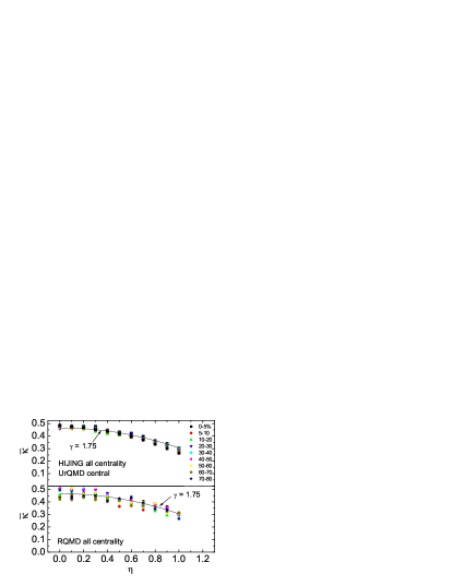
Figure 3: The charge transfer fluctuation is shown as a function of pseudo-rapidity $\eta$. Different symbols represent standard centralities as shown in the symbol legend. These results are from $8,400$ RQMD events for $\sqrt{s}=130\,\hbox{GeV}$ Au-Au collisions and $50,000$ HIJING events at $\sqrt{s}=200\,\hbox{GeV}$. STAR acceptance and efficiency are taken into account in a simple way by restricting $p_{T}>0.1\,\hbox{GeV}$ and also randomly taking out 10 % of the charged particles.

If $dN_{\rm ch}/d\eta$ is constant within the window as is the case for the STAR Au-Au data at RHIC energies, it is clear that $\bar{\kappa}(\eta)$ still varies with $\eta$ even if $\kappa$ itself is constant and such variation is entirely given by the second term in Eq.(9). In Fig.3, we show HIJING, UrQMD and RQMDSorge et al. (1992); Sorge (1995) results at various centralities together with a single component model fit. The calculation is done with the STAR acceptance $\eta_{o}=1$ and $p_{T}>0.1\,\hbox{GeV}$. Also the STAR detection efficiency is taken into account in a simple way by either randomly taking out 10 % of charged particles (for simulations) or by adding 10 % of uncorrelated charged particles (for the neutral cluster model). ¿From these figures, it is clear that the non-QGP model results are very well described by a single-component neutral cluster model with $\gamma\approx 1.75$ independent of centralities. The discrepancy between this value of $\gamma$ and the $\gamma$ obtained in the full phase space study is partly due to the acceptance cuts and partly due to the presence of large $\langle{\Delta Q^{2}}\rangle$ within $|\eta|\leq\eta_{o}$. In the present case of limited observational window, the net charge fluctuations should not be subtracted from $\bar{D}_{u}$.

III A QGP Model – Central Collisions

In RHIC energy heavy-ion reactions, the energy density of the created systems vary with the centrality of the collisions. The results of HIJING simulations and its single-component fit should correspond to the peripheral collision results. In central collisions, one expects that a QGP is formed and is concentrated around midrapidity. Hence, the final state particles can have 2 different origins in central collisions: Some particles will come from the hadronized QGP and others will come from the non-QGP hadronic component of the system.

In Ref.Shi and Jeon (2005) we used a two-component neutral cluster model and showed that even for such an inhomogeneous matter Eq.(9) still holds if one substitutes the $f(\eta^{+},\eta^{-})$ with the following combination of the QGP correlation function $f_{\rm QGP}$ and the hadronic gas correlation function $f_{\rm HG}$

$$f(\eta^{+},\eta^{-})=(1-p)f_{\rm HG}(\eta^{+},\eta^{-})+pf_{\rm QGP}(\eta^{+},\eta^{-})$$ (11)

Here $p$ is the fraction of the charged particles originating from the QGP component in the whole phase space.

Each charge correlation function is assumed to have the separable form as in Eqs.(5) and (6). In the rest of this manuscript, we denote the hadronic correlation length with $\gamma_{1}$ and the QGP correlation length with $\gamma_{2}$. The charge correlation length is expected to be a factor of $2-4$ times smaller in the QGP than in the hadronic matterJeon and Koch (2003), hence, $\gamma_{2}<\gamma_{1}$. The $F(Y)$ functions for each components are chosen as follows.

$$(1-p)F_{\rm HG}(Y) = W(Y)-p\,g_{1}(Y)$$ (12)

$$pF_{\rm QGP}(Y) = p\,g_{2}(Y)$$ (13)

The functions $g_{1}$ and $g_{2}$ are required to satisfy

$$\rho(\eta) = \int_{-\infty}^{\infty}\frac{d\eta^{\prime}}{2\gamma_{1}}\,g_{1}((\eta^{\prime}+\eta)/2)\,e^{-|\eta^{\prime}-\eta|/\gamma_{1}}$$ (14)

$$= \int_{-\infty}^{\infty}\frac{d\eta^{\prime}}{2\gamma_{2}}\,g_{2}((\eta^{\prime}+\eta)/2)\,e^{-|\eta^{\prime}-\eta|/\gamma_{2}}$$

The function $W(Y)$ is again given by the left hand side of Eq.(7) with $\gamma=\gamma_{1}$. The function $\rho(\eta)$ has the meaning of the normalized $dN_{\rm ch}/d\eta$ for the hadrons coming from the QGP component (the dot-dashed line in Fig.1).

For $g_{1}(Y)$ we chose a gaussian

$$g_{1}(Y)=\frac{1}{\sqrt{2\pi\sigma_{1}^{2}}}\,e^{-Y^{2}/2\sigma_{1}^{2}}$$ (15)

which fixes $g_{2}(\eta)$ to be

$$g_{2}(\eta)=\frac{\gamma_{2}^{2}}{\gamma_{1}^{2}}g_{1}(\eta)$$ (16)

$$+\left(1-\frac{\gamma_{2}^{2}}{\gamma_{1}^{2}}\right)\int_{-\infty}^{\infty}\frac{d\eta^{\prime}}{2\gamma_{1}}\,g_{1}((\eta^{\prime}+\eta)/2)\,e^{-|\eta^{\prime}-\eta|/\gamma_{1}}$$

again using the fact that $R_{\rm HG}$ and $R_{\rm QPG}$ are Green functions. The resulting charged particle distribution typically looks like Fig.1.

So far we have introduced 4 parameters, $p,\gamma_{1},\gamma_{2}$ and $\sigma_{1}$. We can fix

$$\gamma_{1}=1.75$$ (17)

by assuming that the HIJING data shown in Fig. 3 is consistent with peripheral collisions at RHIC.For central collisions, we further fix $p$ by requiring that it is the maximum possible value that satisfies $F_{\rm HG}(Y)\geq 0$. This in practice means $p=W(0)/g_{1}(0)$. For peripheral collisions, the QGP fraction $p$ is presumed to be zero.

The remaining 2 parameters $\gamma_{2}$ and $\sigma_{1}$ can be further constrained by considering the experimental data on the net charge fluctuations from STAR Adams et al. (2003). ¿From Ref.Adams et al. (2003), we can infer that for central collisions

$$\bar{\kappa}(\eta_{o}=1.0)\approx 0.27$$ (18)

The results of numerically exploring $0<\gamma_{2}\leq 1.0$ are shown in Fig. 4. At each $\gamma_{2}$, there is a single $\sigma_{1}$ that makes $\bar{\kappa}(1.0)=0.27$. With $\sigma_{1}$ thus fixed, one can then calculate the extent of the QGP component in the pseudo-rapidity space by calculating $p$ and the rms-width

$$\xi=\sqrt{\sigma_{1}^{2}+\gamma_{1}^{2}/2}$$ (19)

of $\rho(\eta)$ (c.f.Eq.(14)). Note that $\xi>\gamma_{1}/\sqrt{2}=1.24$ is always larger than the STAR rapidity window size $\eta_{o}$.

The results of the charge transfer fluctuation calculations in the two-component model are shown Fig. 4. For comparison, we have also plotted results of the single-component model calculations in Fig. 5. The results of the single-component and two-component model calculations are distinctive enough that the measurement of $\bar{\kappa}(\eta)$ can clearly differentiate the two model scenarios, hence providing a way to show the existence of the QGP.

For the two-component model, we find the single data point at $\eta=1.0$ does not constrain the overall shape of $\bar{\kappa}(\eta)$ that much. We can find a range of possible parameter sets that give the same $\bar{\kappa}(1.0)=0.27$ while the corresponding shapes of $\bar{\kappa}(\eta)$ are all very different. The biggest difference among these parameter sets is the value of $\bar{\kappa}(\eta)$ at $\eta=0.0$, where the concentration of the QGP component is strongest. The four lines with $0.001\leq\gamma_{2}\leq 1.0$ in Fig. 4 represent typical results in two-component model calculations.

In a clear contrast, in the single component model the value of $\bar{\kappa}(1.0)$ completely fixes the shape of $\bar{\kappa}(\eta)$ in the entire interval $0.0\leq\eta\leq 1.0$. To have $\bar{\kappa}(1.0)=0.27$, the correlation length must be $\gamma=1.3$. As shown in Ref.Shi and Jeon (2005), $\bar{\kappa}(\eta)$ is proportional to $\gamma$ in the limit $\gamma/\eta_{o}\ll 1$. Hence reduction in $\gamma$ results in the overall reduction of the $\bar{\kappa}(\eta)$ in the whole range.

¿From these considerations, we can say that the measurement of the charge transfer fluctuations in the entire range $0.0<\eta<1.0$ for various centralities will be a critical test for the existence of QGP. If the cental collision data shows a clear reduction from the $\gamma=1.3$ line in Fig. 5, it can only be explained by the presence of the second component. We also expect the amount of QGP would grow as one goes from peripheral to central collisions. Therefore, the most peripheral collision data for $\bar{\kappa}(\eta)$ will behave more like the single-component results while the most central collision data for $\bar{\kappa}(\eta)$ will behave more like the two-component results. We predict that the most central collision data should lie between the two solid lines with $\gamma_{2}=0.6$ and $0.3$ in Fig.4. For comparison, we have also shown two extreme cases with very large and very small QGP charge correlation lengthes where $\gamma_{2}=1.0$ and $0.001$.

In summary, we have made the following prediction for the charge transfer fluctuations within limited pseudo-rapidity range of $|\eta|\leq 1.0$. Suppose that the systems created by two colliding heavy ions at RHIC are inhomogeneous mixtures of the QGP component and the non-QGP hadronic component. Further suppose that the QGP component is concentrated near midrapidity and as one goes from peripheral to central collisions, the amount of the created QGP increases. Then the charge transfer fluctuations, $\bar{\kappa}(\eta)=\bar{D}_{u}(\eta)/(dN_{\rm ch}/d\eta)$, should show the following signature of the presence of the QGP: Going from peripheral to central collisions, $\bar{\kappa}(\eta=0.0)$ should decrease substantially from about 0.45 to 0.35 while $\bar{\kappa}(\eta=1.0)$ should decrease by a small amount from about 0.3 to 0.27. ¿From the amount of the reductions, we can then infer the size and the fraction of the QGP matter. In contrast, if a QGP is not formed at any centralities, then the data points from different centralities should all fall on the same curve.

Figure 4: The results of two-component model calculations together with the single-component result that describes the HIJING data. Also shown is the position of the data point deduced from the STAR net charge fluctuations measurement.

IV Uncorrelated charges

The detection efficiency for charged particles is typically less than 100 % in real experiments. This has been a concern in the measurement of the net charge fluctuations. In the previous paper, we have argued that this effect is small and will not effect the qualitative arguments we had Shi and Jeon (2005). However, with limited observation window, the difference between one and two component model is more quantitative and the detector efficiency deserves some attention.

In terms of the pair correlations, the non-ideal detector efficiency renders some of the correlated pair to be uncorrelated. The relevant formulas are already worked out in the previous paper Shi and Jeon (2005).

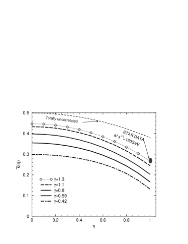
Figure 5: Single-component results. The lower four lines have the same $\bar{\kappa}(1)$ values as the four two-component model results in Fig.4. Also shown are the results for the totally uncorrelated case (upper most line) and the single-component model result that has $\bar{\kappa}(1)=0.27$ (thin line connecting the diamond symbols).

If the detector efficiency is $\epsilon$ and all the charged particles are correlated, then $1-\epsilon$ of detected particles will become uncorrelated because their partners are not detected. The corresponding charge transfer fluctuations are $\bar{\kappa}=\epsilon\bar{\kappa}_{\rm corr}+(1-\epsilon)\bar{\kappa}_{\rm uncorr}$, where $\bar{\kappa}_{\rm corr}$ is for the fully correlated charged particles and $\bar{\kappa}_{\rm uncorr}$ is for the uncorrelated charged particles.

The shape of $\bar{\kappa}_{\rm uncorr}$ is shown in Fig.5. The shape is flatter than the correlated cases and it is always above $\bar{\kappa}_{\rm corr}$. The detector efficiency in STAR experiment is about $85-90\,\%$. Having $10\,\%$ of uncorrelated charges will slightly increase $\bar{\kappa}(\eta)$ and make the overall shape a little bit flatter. This, however, will not change much of the results for $\kappa(\eta)$. The signature for the appearance of the second QGP-like component is still present, and we can still put an upper limit on the $\gamma_{\rm QGP}$ if a significant reduction of $\kappa(0.0)$ is observed. All the results presented in this paper already considered the effect of uncorrelated charged particles.

V Summary

In this paper, we proposed the charge transfer fluctuation as a good observable capable of detecting the local presence of a QGP in a limited pseudo-rapidity space. In contrast, the net charge fluctuationsAsakawa et al. (2000); Jeon and Koch (2000) and the width of the balance functionBass et al. (2000) are only sensitive to the presence of a QGP when the fraction of the QGP component is substantial in the whole observational window. Since longitudinal inhomogeneity is expected from both theoretical considerations and experimental observations, it is important to have an observable that is sensitive to it. Furthermore, such inhomogeneity may explain why the net charge fluctuations did not show a strong signal even though the underlying net charge fluctuations could be strongly reduced in the QGP phase.

In this study, we showed that the three hadronic models, HIJING, RQMD and UrQMD are consistent with a single-component model with fixed charge correlation length of about about $\gamma=1.75$. If a QGP is created in central heavy ion collisions, a significant deviation from this behavior is expected in the data. Specifically, if the QGP component is concentrated around the midrapidity and tapers off going away from midrapidity, then one should see the following trends in the data:

1. The overall values of $\bar{\kappa}(\eta)$ must decrease going from peripheral collisions to central collisions. This indicates that more QGP is being created.

2. The value of $\bar{\kappa}(1.0)$ should change moderately from around 0.30 to 0.27 from peripheral to central collisions. These values correspond to the HIJING, UrQMD and RQMD value for peripheral Au-Au collisions, and the measured value of $\langle{\Delta Q^{2}}\rangle/\langle{N_{\rm ch}}\rangle$ for central Au-Au collision from STAR. This small reduction indicates that near $\eta=\pm 1$, the contribution from the QGP component is already much reduced.

3. The reduction in the value of $\bar{\kappa}(0.0)$ should be larger than the reduction in the value of $\bar{\kappa}(1.0)$ as the QGP component is more concentrated around midrapidity. Going from peripheral to central events, the value of $\bar{\kappa}(0.0)$ should vary from around 0.45 (HIJING, UrQMD, RQMD) down to 0.35. The value of $\bar{\kappa}(0.0)$ puts a severe constraint on the value of the charge correlation length for the QGP component.

The change in the value of $\bar{\kappa}(0.0)$ may not seem large. But keep in mind that the value of $\bar{\kappa}(1.0)$ cannot be lower than the already measured value of $0.27$. Hence $\bar{\kappa}(0.0)$, too, cannot go lower than that. If $\bar{\kappa}(0.0)$ is measured to be close to 0.35, it is impossible to explain this without the presence of the second phase with a very short charge correlation length.

In summary, we propose that the charge transfer fluctuation is a sensitive observable to find the presence and extent of the QGP created in high energy heavy ion collisions. In addition, this observable is relatively easy to measure and does not require the net charge conservation correction. We strongly suggest the experimental group to measure the charge transfer fluctuations.