The Fubini-Furlan-Rosetti sum rule and related aspects in light of covariant baryon chiral perturbation theory

Abstract

We analyze the Fubini-Furlan-Rosetti sum rule in the framework of covariant baryon chiral perturbation theory to leading one–loop accuracy and including next-to-leading order polynomial contributions. We discuss the relation between the subtraction constants in the invariant amplitudes and certain low-energy constants employed in earlier chiral perturbation theory studies of threshold neutral pion photoproduction off nucleons. In particular, we consider the corrections to the sum rule due to the finite pion mass and show that below the threshold they agree well with determinations based on fixed-$t$ dispersion relations. We also discuss the energy dependence of the electric dipole amplitude $E_{0+}$.

1 Introduction

The Fubini-Furlan-Rosetti (FFR) sum rule was derived in the sixties utilizing the soft-pion techniques of current algebra FFR . It relates the nucleon anomalous magnetic moment to an integral over the invariant amplitude $A_{1}$ of pion photoproduction

$$\kappa^{v,s}=\frac{8m_{N}^{2}}{e\pi g_{\pi N}}\,\int\frac{d\nu^{\prime}}{\nu}\,{\rm Im}~{}A_{1}^{(+,0)}(\nu^{\prime},t=0)~{},$$ (1)

if one utilizes the Goldberger-Treiman relation $g_{A}m_{N}=\\ F_{\pi}g_{\pi N}$, with $m_{N}$ the nucleon mass, $g_{A}$ the axial-vector coupling constant, $F_{\pi}$ the weak pion decay constant and $g_{\pi N}$ the strong pion–nucleon coupling constant. Furthermore, $\kappa^{v}=\kappa_{p}-\kappa_{n}$ and $\kappa^{s}=\kappa_{p}+\kappa_{n}$ are the nucleon isovector and isoscalar anomalous magnetic moment, respectively. The FFR sum rule is exact in the chiral limit of QCD and thus all quantities appearing in Eq. (1) are to be understood in the limit of vanishing light quark masses, $m_{q}=0$. The FFR sum rule has recently been reexamined in Ref. PDT . In that paper, pion mass corrections to the sum rule were considered (in terms of a discrepancy function $\Delta_{N}(\nu,t)$) and numerical evaluations based on a) dispersion relations and b) input from heavy baryon chiral perturbation theory (HBCHPT) were presented. It was pointed out that in the strict framework of HBCHPT the nucleon pole positions are slightly moved, which leads e.g. to an incorrect curvature of the discrepancy function for energies below the threshold. A similar behavior due to the shift of pole or cut positions in the $1/m_{N}$ expansion was observed already in the discussion of the Compton cusp at the opening of the pion threshold BKMS , the spectral functions of the nucleon isovector form factors BKMspec or the scalar form factor of the nucleon BL . Note, however, that the kinematical factors leading to the corresponding poles or cuts need not be expanded in HBCHPT as it is discussed e.g. in Ref. BKMS . Clearly, in a manifestly Lorentz-invariant formulation of baryon CHPT such problems do not arise, see e.g. BL ; KM ; MZrel . The purpose of this paper is two-fold: We analyze the FFR sum rule in the framework of infrared regularization (IR) of baryon CHPT BL and demonstrate that the energy dependence of the discrepancy function is correctly given. Second, we also take a closer look at the pion mass corrections to the sum rule, which can only be systematically calculated in chiral perturbation theory, and the related threshold multipoles in pion photoproduction. Our calculation includes all terms at third order in the chiral expansion and in addition, also the fourth order polynomial terms in the photoproduction amplitudes. Our aim is to show that within IR baryon CHPT one can describe pion photoproduction above and below threshold and that the dispersive representation can indeed be used to pin down certain low–energy constants (LECs), as suggested in PDT . It is well-known that the chiral expansion converges best in the unphysical region where all momenta can be very small. Consequently, in such regions LECs can be determined to a good precision if a corresponding dispersive representation is available. A more refined treatment including all fourth order terms and fits to the existing low–energy data from MAMI will be relegated to a future publication.

The manuscript is organized as follows: In Sec. 2 we briefly recall the formalism of pion photoproduction and collect some results for the pion mass corrections to the FFR sum rule derived in PDT . We also present an alternative way of looking at these. Sec. 3 contains the results on the FFR sum rule, the discrepancy function and the related electric dipole amplitude $E_{0+}$ as well as the slopes of the P-wave multipoles at threshold. We demonstrate that one can indeed determine LECs from the amplitudes in the unphysical region and end with a brief outlook.

2 Formalism

Consider pion photoproduction off the nucleon by real photons with $k^{2}=0$

$$\gamma(k)+N(p_{1})\to\pi^{a}(q)+N(p_{2})~{},$$ (2)

where $p_{1}\,(p_{2})$ is the four–momentum of the incoming (outgoing) nucleon ($N$) and $a$ an isospin index ($a=+,0,-$). For the discussion of the FFR sum rule, only the isospin $0$ and $+$ channels are of relevance, i.e. the physical channels $\gamma p\to\pi^{0}p$ and $\gamma n\to\pi^{0}n$. The corresponding S-matrix is given in terms of four invariant functions $A_{i}$ ($i=1,\ldots,4$) that depend on two kinematical variables. Throughout, we utilize the notation of our earlier work Relphoto2 and refer to that reference for a detailed discussion of the pertinent formalism. These invariant amplitudes can be calculated in baryon chiral perturbation theory and have the generic form (we do not display isospin quantum numbers and kinematical arguments)

$$A_{i}=A_{i}^{\rm Born}+A_{i}^{\rm loop}+A_{i}^{\rm ct}~{},$$ (3)

where the Born terms subsume the coupling to the charge and the magnetic moment of the nucleon (note often the alternative notation of “pole terms” is used for these contributions – sometimes even calculated employing the pseudoscalar pion-nucleon coupling). All further counter terms are collected in the polynomial terms $A_{i}^{\rm ct}$. The non-trivial loop contributions (after renormalization of the single nucleon properties) are collected in the $A_{i}^{\rm loop}$. In Ref. Relphoto2 , the $A_{i}$ were calculated to third order (leading loop order) in relativistic baryon CHPT. In that formulation, a violation of the power counting through the nucleon mass term is manifest. However, from the integral representations given in Relphoto2 , it is straightforward to isolate the so-called infrared singular part BL that contains the chiral long–distance physics and leads to a one-to-one correspondence between the expansion in loops and small momenta/pion masses. This can e.g. be achieved by the prescription given in BL which we also will employ. Symbolically, it reads $\int_{0}^{1}dx\to(\int_{0}^{\infty}-\int_{1}^{\infty})dx=I+R$, with $I$ and $R$ the infrared singular (irregular) and the regular part, respectively. For the study of the FFR sum rule and related aspects, we are interested in the amplitudes at small energies and momentum transfer and thus use the variables $\nu=(s-u)/4m_{N}$ and $\nu_{B}=-(s+u-2m_{N}^{2})/4m_{N}$, which are odd and even under crossing $s\leftrightarrow u$ (for further notation, see Relphoto2 ). From the crossing properties of the $A_{i}$ and their low-energy properties as detailed in Relphoto2 , one derives the following representation for the polynomial pieces (note in particular the low-energy theorem for $A_{1}$ Relphoto1 that forbids a constant term)

$$A_{1}^{\rm ct} = a_{1}^{1}\nu^{2}+a^{2}_{1}\nu_{B}+\ldots~{},$$

$$A_{2}^{\rm ct} = a_{2}^{0}+\ldots~{},$$

$$A_{3}^{\rm ct} = a_{3}^{1}\nu+\ldots~{},$$

$$A_{4}^{\rm ct} = a_{4}^{0}+\ldots~{}.$$ (4)

At third order in the chiral expansion, only the leading term of $A_{4}$ contributes Relphoto2 , whereas all other terms written down in Eq. (2) start at ${\cal O}(q^{4})$. The mapping between these subtraction constants and the low-energy constants (LECs) used in the heavy baryon calculations HBphoto1 ; HBphoto2 ; HBphoto3 is given in the appendix. We remind the reader that although the contribution of $A_{1}^{\rm ct}$ formally starts as $M_{\pi}^{2}$ at threshold, in the chiral limit the expansion coefficients are singular leading to the famous contribution to the low-energy theorem for the threshold value of $E_{0+}$ at next-to-leading order in the pion mass expansion Relphoto1 . We note that $A_{2}^{\rm ct}$ only feeds into the P-wave slope $\bar{P}_{2}$ and into the D-wave at threshold in such a way that it cancels in the FFR sum rule at finite pion mass. Therefore, the subtraction constant $a_{2}^{0}$ has to be determined completely independently of the FFR sum rule, say by fitting to the slope of $P_{2}$ at threshold. In the following, we use the third order IR representation of the pertinent one-loop graphs (which contains an infinite series of $1/m_{N}$ corrections in the heavy baryon framework) but also use the fourth-order subtraction constants displayed in Eq. (2). Based on that representation, we attempt a simultaneous description of the $\nu$-dependence of the FFR discrepancy function $\Delta_{p}(\nu,t_{\rm thr})$ (as defined below), the energy dependence of the electric dipole amplitude $E_{0+}$ for neutral pion production off protons and the P–wave threshold slopes as extracted in E0pdata . Similarly precise information is not available for the neutron, therefore in the following we mostly concentrate on the proton.

In Ref. PDT , the FFR sum rule was considered for finite mass pions and the following representation in terms of a discrepancy function $\Delta_{N}$ was derived:

$$\stackrel{{\scriptstyle\circ}}{{\kappa}}_{N}\tau_{3}+\Delta_{N}(\nu,t_{\rm thr})$$

$$\quad=\frac{4m_{N}^{2}}{e\pi g_{\pi N}}\,\int_{\nu_{\rm thr}}^{\infty}\frac{d\nu^{\prime}}{\nu}\,\frac{\nu^{\prime}\,{\rm Im}~{}A_{1}^{(N,\pi^{0})}(\nu^{\prime},t=t_{\rm thr})}{{v^{\prime}}^{2}-\nu^{2}}~{},$$

$$\Delta_{N}(\nu,t=t_{\rm thr})$$

$$\quad=\frac{2m_{N}^{2}}{eg_{\pi N}}\,\left(A_{1}^{\rm loop}(\nu,t=t_{\rm thr})+A_{1}^{\rm ct}(\nu,t=t_{\rm thr})\right).$$ (5)

A few comments on this equation are in order. First, the left-hand-side of the FFR sum rule gives the anomalous magnetic moment in the chiral limit, $\kappa_{N}=\stackrel{{\scriptstyle\circ}}{{\kappa}}_{N}+{\cal O}(m_{q}^{1/2})$. Therefore, if one uses the physical value of $\kappa_{N}$ as in Ref. PDT , one must include the corresponding loop and counter term corrections into the discrepancy function. However, for studying the pion mass corrections to the FFR sum rule, it is more appropriate to work with the chiral limit values of $\kappa_{p}$ and $\kappa_{n}$, as discussed below. Second, in the chiral limit, $t\to 0$. This value can, of course, not be achieved in the physical world. We follow PDT and present our results at the minimal (threshold) value of $t$, $t_{\rm thr}=-M_{\pi}^{2}/(1+M_{\pi}/m)=-0.016\,$GeV^-2. Third, the Goldberger-Treiman relation is no longer exact at finite pion mass, to the order we are working, it takes the form GSS ; FMS

$$\frac{g_{\pi N}}{m_{N}}=\frac{g_{A}}{F_{\pi}}\left(1-\frac{2M_{\pi}^{2}}{g_{A}}\bar{d}_{18}\right)\,,$$ (6)

with $\bar{d}_{18}$ a LEC. As long as one only works at the physical pion mass, this effect is taken care of by utilizing the physical value for the pion–nucleon coupling and the nucleon mass. If one, however, also wants to study the pion mass dependence of $\Delta_{N}$, as will be done here, one explicitly has to include this pion mass dependence. However, this effect only shows up in the terms cubic in the pion mass, which will not be considered in detail here (for a more detailed discussion of this topic, see e.g. EGM ). Note this pion mass dependence can only be systematically calculated in chiral perturbation theory and, eventually, in lattice QCD.

We have explicitly worked out the quark mass expansion of the discrepancy function at threshold. For the proton, it takes the form (modulo chiral logs)

$$\Delta_{p}(\nu=\nu_{\rm thr},t=t_{\rm thr})=\alpha_{p}M_{\pi}+\beta_{p}M_{\pi}^{2}+\ldots$$ (7)

with

$$\alpha_{p} = \frac{m_{N}}{16F_{\pi}^{2}}\,\left(1-\frac{4g_{A}^{2}}{3\pi}\right)~{},$$

$$\beta_{p} = \frac{1}{8\pi^{2}F_{\pi}^{2}}\biggl{[}-3-\frac{\pi^{2}}{8}+\bigl{(}7-\frac{1}{2}\stackrel{{\scriptstyle\circ}}{{\kappa}}_{p}+\frac{1}{2}\stackrel{{\scriptstyle\circ}}{{\kappa}}_{n}\bigl{)}\ln\frac{M_{\pi}}{m_{N}}\biggr{]}$$ (8)

$$- \frac{g_{A}^{2}}{48\pi^{2}F_{\pi}^{2}}\biggl{[}-\frac{85}{3}-\pi+\frac{5}{3}\stackrel{{\scriptstyle\circ}}{{\kappa}}_{p}-\frac{11}{3}\stackrel{{\scriptstyle\circ}}{{\kappa}}_{n}$$

$$\qquad\qquad\qquad\qquad+(5+7\stackrel{{\scriptstyle\circ}}{{\kappa}}_{p}-\stackrel{{\scriptstyle\circ}}{{\kappa}}_{n})\ln\frac{M_{\pi}}{m_{N}}\biggr{]}$$

$$+ \frac{\tilde{c}_{4}}{6\pi^{2}F_{\pi}^{2}}\left(-\frac{10}{3}+\frac{3\pi^{2}}{8}+\frac{5}{2}\ln\frac{M_{\pi}}{m_{N}}\right)$$

$$- 8m_{N}(2e_{105}+e_{106})+\frac{2m_{N}F_{\pi}}{g_{A}}\left(a_{1}^{1}-\frac{a_{1}^{2}}{2m_{N}}\right)~{},$$

where $\tilde{c}_{4}=m_{N}\,c_{4}$ and $c_{4}=3.4\,$GeV^-1 BM . The LECs $e_{105}$ and $e_{106}$ from the dimension four chiral pion-nucleon Lagrangian contribute to the proton and neutron anomalous magnetic moment at next-to-leading loop order (for a detailed discussion, see KM ). Their values are discussed below. Further, we have set the scale of dimensional regularization equal to the nucleon mass, $\lambda=m_{N}$. Of course, $\Delta_{p}$ vanishes in the chiral limit. Notice the absence of chiral logs in the terms linear in the pion mass. The representation of $\Delta_{p}$ given Eq. (7) is exact to fourth order in the chiral expansion since it can be reconstructed from the HBCHPT results obtained in HBphoto1 ; HBphoto2 ; HBphoto3 . In addition, to arrive at these results, we had to include the small contribution from the slope of the D-wave combination $D=M_{2+}-E_{2+}-P_{2-}-E_{2-}$, that is $\bar{D}=D/q^{2}$ at threshold. It is obtained from the invariant functions by

$$D(s)=\frac{5}{16}\,\int dx~{}(x^{4}-2x^{2}+1)\,{\cal F}_{4}(s,x)~{},$$ (9)

with ${\cal F}_{4}(s,x)$ a combination of $A_{2,3,4}$, see Relphoto2 . This contribution has not been calculated before. Note further that Eq. (7) includes the terms that renormalize $\stackrel{{\scriptstyle\circ}}{{\kappa}}_{p}$ to its physical value, $\kappa_{p}$, since we identify the left-hand-side of the FFR with the anomalous magnetic moment in the chiral limit. The pion mass expansion of $\Delta_{n}(\nu=\nu_{\rm thr},t=t_{\rm thr})$ looks very similar, we find

$$\alpha_{n} = \frac{m_{N}}{16F_{\pi}^{2}}\,\left(1-\frac{4g_{A}^{2}}{3\pi}\right)~{},$$

$$\beta_{n} = -\frac{1}{8\pi^{2}F_{\pi}^{2}}\biggl{[}\frac{7}{9}+\frac{\pi^{2}}{8}+\bigl{(}-\frac{13}{3}+\frac{1}{2}\stackrel{{\scriptstyle\circ}}{{\kappa}}_{p}-\frac{1}{2}\stackrel{{\scriptstyle\circ}}{{\kappa}}_{n}\bigr{)}\ln\frac{M_{\pi}}{m_{N}}\biggr{]}$$ (10)

$$- \frac{g_{A}^{2}}{48\pi^{2}F_{\pi}^{2}}\biggl{[}-\frac{76}{3}-\pi+\frac{11}{3}\stackrel{{\scriptstyle\circ}}{{\kappa}}_{p}-\frac{5}{3}\stackrel{{\scriptstyle\circ}}{{\kappa}}_{n}$$

$$\qquad\qquad\qquad\qquad+(-1+\stackrel{{\scriptstyle\circ}}{{\kappa}}_{p}-7\stackrel{{\scriptstyle\circ}}{{\kappa}}_{n})\ln\frac{M_{\pi}}{m_{N}}\biggr{]}$$

$$- \frac{\tilde{c}_{4}}{6\pi^{2}F_{\pi}^{2}}\left(-\frac{10}{3}+\frac{3\pi^{2}}{8}-\frac{5}{2}\ln\frac{M_{\pi}}{m_{N}}\right)$$

$$+ 8m_{N}(2e_{105}-e_{106})+\frac{2m_{N}F_{\pi}}{g_{A}}\left(a_{1}^{1,n}-\frac{a_{1}^{2,n}}{2m_{N}}\right)~{},$$

where the subtraction constants refer to the neutron amplitude $\gamma n\to\pi^{0}n$ as denoted by the superscript $n$.

3 Results

First, we must fix our input parameters. We use $F_{\pi}=92.4\,$MeV, $M_{\pi^{+}}=139.57\,$MeV, $M_{\pi^{0}}=134.97\,$MeV, $m_{p}=938.27\,$MeV, $m_{n}=939.57\,$MeV, $g_{\pi N}=13.4$, $\kappa_{p}=1.793$, $\kappa_{n}=-1.913$. To the order we are working, the anomalous magnetic moment of the proton and the neutron are given in terms of two LECs from the dimension two chiral Lagrangian commonly denoted $c_{6}$ and $c_{7}$ and loop corrections that start with terms of order $M_{\pi}^{3}$ BKMlec . From that one can read off the chiral limit values for the proton and the neutron anomalous magnetic moments,

$$\stackrel{{\scriptstyle\circ}}{{\kappa}}_{p}=2.37~{},~{}~{}\stackrel{{\scriptstyle\circ}}{{\kappa}}_{n}=-2.84~{},$$ (11)

in nuclear magnetons. For comparison, at third order in HBCHPT, we have $\stackrel{{\scriptstyle\circ}}{{\kappa}}_{p}=2.85$, $\stackrel{{\scriptstyle\circ}}{{\kappa}}_{n}=-2.98$ BKMlec .

The overall best fit to simultaneously describe the proton discrepancy function, the electric dipole amplitude in the threshold region and the three P-wave slopes is obtained with the following polynomial contribution to the invariant functions

$$A_{1}^{\rm ct}(\nu,\nu_{B}) = (191.3\nu_{B}+220\nu^{2})~{}\mbox{GeV}^{-2}~{},$$

$$A_{2}^{\rm ct}(\nu,\nu_{B}) = -54.9~{}\mbox{GeV}^{-4}~{},$$

$$A_{3}^{\rm ct}(\nu,\nu_{B}) = -155\nu~{}\mbox{GeV}^{-3}~{},$$

$$A_{4}^{\rm ct}(\nu,\nu_{B}) = 181.5~{}\mbox{GeV}^{-3}~{}.$$ (12)

While these coefficients appear large at first glance, in the appendix we show that they match quite nicely the corresponding LECs determined in fits to neutral pion photoproduction differential cross sections and the photon asymmetry. Since the LECs can be understood to a good precision in terms of resonance saturation (excitation of the $\Delta(1232)$ and of vector mesons, see e.g. HBphoto1 ), the numbers appearing in Eq. (3) are indeed of natural size. The resulting threshold values for $E_{0+}$ and the $\bar{P}_{i}$ ($i=1,2,3$) are

$$E_{0+} = -1.19\,~{}~{}[-1.23\pm 0.08\pm 0.03]~{},$$

$$\bar{P}_{1} = \phantom{-}9.67\,~{}~{}[9.46\pm 0.05\pm 0.28]~{},$$

$$\bar{P}_{2} = -9.6\,~{}~{}[-9.5\pm 0.09\pm 0.28]~{},$$

$$\bar{P}_{3} = \phantom{-}11.45\,~{}[11.32\pm 0.11\pm 0.34]~{},$$ (13)

in the conventional units of $10^{-3}/M_{\pi^{+}}$ and $10^{-3}/M_{\pi^{+}}^{2}$, respectively. The experimental numbers in the square brackets are from E0pdata . We note that $\bar{P}_{2}$ is obtained by adjusting the subtraction constant $a_{2}^{0}$. The corresponding D-wave slope is

$$\bar{D}=0.66\cdot 10^{-3}/M_{\pi^{+}}^{3}~{},$$ (14)

to be compared with 0.96 (0.92) from the MAID03 analysis (the dispersive analysis of Ref. HDT ).

Let us look at these results in more detail. For the pion mass correction to the proton FFR sum rule, we find

$$\stackrel{{\scriptstyle\circ}}{{\kappa}}_{p}+\Delta_{p}(\nu=\nu_{\rm thr},t=t_{\rm thr})=2.18~{}$$ (15)

which should be compared with the left-hand-side of the sum rule, i.e. the proton anomalous magnetic moment in the chiral limit, cf. Eq. (11). Thus, within this framework, the FFR sum rule is fulfilled within 8%, which is of the expected size since pion mass effects are proportional to the small parameter $\mu=M_{\pi}/m_{N}\simeq 1/7$. Note again that this way of looking at the FFR differs from what was done in PDT , where the left-hand-side of the FFR was identified with the physical value of the proton anomalous magnetic moment and the discrepancy function defined there thus differs from ours by terms $\sim\stackrel{{\scriptstyle\circ}}{{\kappa}}_{p}-\kappa_{p}$.

Next, we display the resulting discrepancy function for the proton as a function of $\nu$ at fixed $t=t_{\rm thr}$ in Fig. 1 (for better comparison with Ref. PDT , this discrepancy function is taken with respect to the physical value of the proton anomalous magnetic moment).

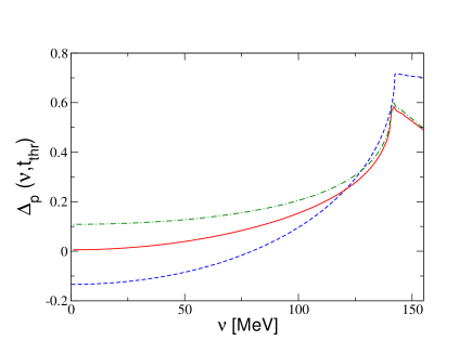
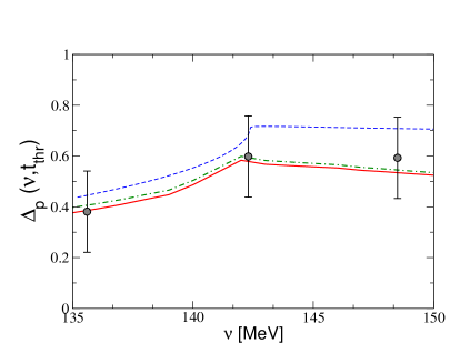
Figure 1: The discrepancy function $\Delta_{p}$ for the proton. Solid line: IR baryon CHPT. Dot-dashed line: third order relativistic CHPT Relphoto2 . Dashed line: Dispersive result based on the MAID model, from PDT . Upper panel: $\nu$ in the range from 0 to 155 MeV. lower panel: Threshold region (135 MeV$\leq\nu\leq$150 MeV). The data points are calculated with the S- and P-wave multipoles from Ref. E0pdata (based on the formalism developed in PDT ).

At $\nu=0$, the discrepancy functions has indeed an extremum (as pointed out in PDT ) and it increases with increasing $\nu$. We also find the pronounced cusp effect at $\nu=\nu_{\rm thr}$, as it is expected. In contrast to the prediction based on the MAID model (dashed curved), we do not observe any zero crossing for the values of the subtraction constants given in Eq. (3). Naturally, within our approach we should have a band rather than a line but we relegate a detailed error analysis to a later work, when we will also fit to all data of neutral pion photoproduction in the threshold region. Interestingly, the third order relativistic result from Relphoto2 (dot-dashed line) is very close to the IR result including the fourth order polynomial pieces. We also note that the incorrect behavior at $\nu\simeq 0$ observed in the HBCHPT calculation is of course not present in our manifestly covariant calculation, as it was suggested already in PDT . Note furthermore that we do not show $\Delta_{P}(\nu,t_{\rm thr})$ for values of $\nu>155\,$MeV because at $\nu\simeq 170\,$MeV, a steep rise due to the $\Delta(1232)$ resonance sets in PDT . In the lower panel of Fig. 1 we focus on the threshold (cusp) region. We see that the relativistic and IR predictions are in good agreement with the MAID model and also with the data reconstructed form the multipoles of Ref. E0pdata (for details, see again PDT ).

We briefly discuss the pion mass dependence of $\Delta_{p,n}$; for this purpose, we switch back to the full fourth order representation obtained from earlier heavy baryon results. Consider the proton. We find for the coefficients in Eq. (7)

$$\alpha_{p} = 2.19~{}{\rm GeV}^{-1}~{},$$

$$\beta_{p} = (-5.0-17.3)~{}{\rm GeV}^{-2}=-22.3~{}{\rm GeV}^{-2}~{},$$ (16)

where we have used the physical values for $g_{A}$ and $F_{\pi}$ and the second term in $\beta_{p}$ is the contribution from the dimension four operators with the LECs $e_{105}$ and $e_{106}$. These counterterms determine the slope of $\kappa_{v}$ and $\kappa_{s}$ in the soft pion limit. Their values have been determined by using the fourth order formula for the anomalous magnetic moment from KM as chiral extrapolation functions for the lattice QCD data of FFlat . We get $e_{105}\simeq 0.45\,,\,e_{106}\simeq 1.4$ at $\lambda=m_{N}$, which are of natural size. Since these are only very rough fits to the trend of the lattice data at too high pion masses, we refrain from assigning a theoretical uncertainties to these numbers. Note that in case of the coefficient $\beta_{p}$, we have large cancellations between the loop and the counterterm contributions proportional to the LECS $c_{i}$, which are $-21.2\,$GeV^-2 and $16.2\,$GeV^-2, respectively, for $\lambda=m_{N}$. We also stress that the first two terms in the quark mass expansion of $\Delta_{p}$ at threshold give $-0.13$, which is to be compared with the full calculation that gives $-0.19$, cf. Eq. (15) (where the contribution from the term $\sim 2e_{105}+e_{106}$ is $-0.34$). For the neutron, we have no determination of the photoproduction counter terms and thus we can only give $\alpha_{n}=\alpha_{p}=2.19\,$GeV^-1 and $\beta_{n}^{\rm loop}=-18.23\,$GeV^-2. This value is comparable to the one of the proton. The contribution from the operators $\sim e_{105},e_{106}$ is somewhat smaller than for the proton since for the neutron they appear with a different relative sign.

Also well described is the energy dependence of the electric dipole amplitude $E_{0+}(E_{\gamma})$ shown in Fig. 2 (with $E_{\gamma}=\nu-(t-M_{\pi}^{2})/4m_{N}$). This description of the data is as good as the complete fourth-order HBCHPT calculation (see e.g. Fig. 3 in E0pdata ). This is not surprising since the third-order IR calculation generates all fourth-order HB corrections with fixed coefficients (from the expansion of the Dirac propagator) and these are the only fourth order loop contributions since loops with one insertion proportional to the dimension two LECs $c_{i}$ do not contribute. Related to this is the observation that most of the non-trivial energy-dependence is given by the generalized cusp function HBphoto1 ; HBphoto3

$$E_{0+}(E_{\gamma})=a+b\sqrt{1-\left(\frac{E_{\gamma}}{E_{\gamma}^{\rm thr}}\right)^{2}}~{},$$ (17)

where the parameter $b$ is proportional to the charge exchange scattering length $a(\pi^{0}p\to\pi^{+}n)$ (see also the detailed discussion in aron1 ; aron2 ).

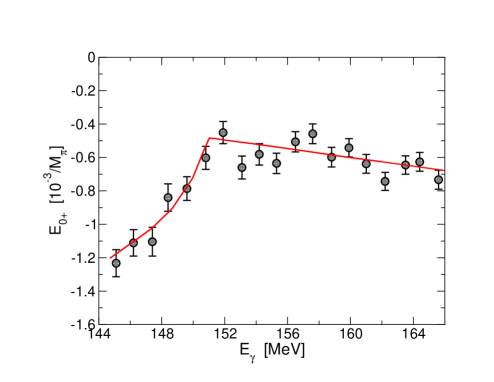
Figure 2: The real part of the electric dipole amplitude $E_{0+}$ in the threshold region. The solid line is the theoretical prediction as discussed in the text and the data are from Ref. E0pdata .

As noted before, similarly precise information on the neutron is not available. The predictions for the threshold multipoles are based on resonance saturation, the only experimental information is from the SAL experiment on $\gamma d\to\pi^{0}d$ SAL that is consistent with the CHPT prediction $|E_{0+,\rm thr}^{\pi^{0}n}|>|E_{0+,\rm thr}^{\pi^{0}p}|$ BBLMvK . We can fit to the energy-dependence of $A_{1}^{n}$ as predicted by the MAID model and the threshold multipoles as predicted by CHPT, but in the absence of more information on the energy dependence of e.g. the neutron electric dipole amplitude and any experimental verification of the predictions for the P–wave slopes based on resonance saturation, the resulting numbers are highly model-dependent and we thus refrain from showing them here.

4 Summary and outlook

In this paper, we have studied the FFR sum rule in the framework of covariant baryon chiral perturbation theory, extending some of the work presented in PDT . We have worked out the loop corrections to third order in the chiral expansion, corresponding to the leading loop contribution, supplemented by the polynomial pieces up-to-and-including fourth order. Since the (sub-)threshold energies considered here are small, such a procedure is justified and would only lead to a readjustment of the subtraction constants defined in Eq. (2) if one includes also the fourth order loop graphs. We have shown that within this framework one can achieve a good description of the energy dependence of the discrepancy function for the proton, defined in Eq. (2), together with the energy dependence of the electric dipole amplitude in the threshold region, cf. Fig. 2, and the P-wave slopes at threshold, see Eq. (3). The corresponding subtraction constants collected in Eq. (3) can be matched to the low-energy constants determined previously in HBCHPT studies of threshold neutral pion photoproduction and their resulting values are of natural size (as detailed in the appendix). We find that the finite pion mass corrections to the FFR sum rule for the proton are small, of the order of 8 % (cf. Eq. (15)). As shown in Fig. 1, the $\nu$-dependence of the discrepancy function for the proton has the proper behavior and agrees with the result of the MAID model. The unphysical behavior observed at $\nu\simeq 0$ in the heavy baryon scheme PDT is absent in a covariant formulation as presented here. It is also interesting to note that the third order relativistic calculation free of counter terms from Relphoto2 also gives a good description of $\Delta_{p}(\nu,t_{\rm thr})$. These findings corroborate the conjecture made in Ref. PDT that one can use the dispersive representation of the invariant amplitudes in the unphysical region to pin down low-energy constants of chiral perturbation theory (see also the appendix). It will be interesting to perform a complete fourth-order calculation and fit the corresponding LECs to the existing unpolarized and polarized threshold data of the reaction $\gamma p\to\pi^{0}p$. This should further sharpen the conclusions made here. Work along such lines is under way BKMfull .

Appendix A Subtraction and low-energy constants

Here, we give the mapping between the commonly employed counter terms of the heavy baryon approach and the subtraction constants defined in Eq.(2). To third order, one has only one P–wave counter term (with the LEC $b_{p}$) that feeds into the multipole $P_{3}$ HBphoto1 ,

$$a_{4}^{0}=4\pi\,b_{P}~{}.$$ (18)

At fourth order, there are two S–wave counter terms (which in the threshold region essentially act as one constant) HBphoto1 . The corresponding LECs $a_{1}$ and $a_{2}$ are given by the following combinations of subtraction constants:

$$12\pi\,a_{1} = -\left(a_{2}^{0}+\frac{a_{4}^{0}}{m_{N}}\right)~{},$$

$$12\pi\,a_{2} = \left(3a_{3}^{1}+a_{2}^{0}+3a_{1}^{1}-\frac{3}{2}\frac{a_{1}^{2}}{m_{N}}+\frac{5}{2}\frac{a_{4}^{0}}{m_{N}}\right)~{}.$$ (19)

Note that in the sum $a_{1}+a_{2}$, the contribution from $A_{2}$ cancels (as noted earlier) and that these relations are to be taken at $\lambda=m_{N}$. Similarly, at fourth order there are two independent counter terms (with the LECs $\xi_{1}$ and $\xi_{2}$) that modify the P-waves $P_{1}$ and $P_{2}$ HBphoto3

$$\frac{a_{1}^{2}}{2}-m_{N}a_{3}^{1}-a_{4}^{0} = \frac{g_{A}}{16\pi^{2}F_{\pi}^{3}}~{}\xi_{1}~{},$$

$$\frac{a_{4}^{0}}{2}+m_{N}a_{3}^{1}-m_{N}a_{2}^{0} = \frac{g_{A}}{16\pi^{2}F_{\pi}^{3}}~{}\xi_{2}~{}.$$ (20)

At first glance, one might conclude from Eqs.(A,A) that there is a mismatch in the number of subtraction constants and counter terms. Note, however, that various subtraction constants feed into the S- and the P-waves so that finally only two independent structures remain for the S-wave and two for the P-waves.

It is interesting to compare the numbers derived from Eq. (3) with the earlier determinations of these counter terms in the HBCHPT framework. Note, however, that we did not include all fourth order loop corrections here, so that the values of the subtraction constants effectively subsume some of these effects. This is not the case for the LEC $b_{P}$ since it already appears at third order. Our value for $a_{0}^{4}$ translates into $b_{P}=14.4\,$GeV^-3. This compares well with the third order fits of Ref. HBphoto1 , $b_{P}=(15.8\pm 0.2)\,$GeV^-3, and of Ref. HBphoto2 , $b_{P}=13.0\,$GeV^-3. Note that the corresponding value in HBphoto3 comes out smaller due to additional loop effects. Consider next the LECs contributing to the electric dipole amplitude in the threshold region. We get $4\pi m_{N}(a_{1}+a_{2})=56.2\,$GeV^-3 from the constants in Eq. (3) compared to 31.8 GeV^-3, 77.8 GeV^-3 and 71.2 GeV^-3 from HBphoto1 , HBphoto2 and HBphoto3 , respectively. Individually, we have $a_{1}=-3.67\,$GeV^-3 and $a_{2}=8.43\,$GeV^-3, which is different from but comparable in size to the free and resonance fits to the various sets of Mainz and Saskatoon data (compare e.g. table 1 in HBphoto3 ). As it was already stressed in these earlier papers, the LECs $a_{1}$ and $a_{2}$ can not be well determined individually from fits to the data in the threshold region. Next, consider the P-wave $P_{1}$. The determination of $\xi_{1}=16.6$ in HBphoto3 translates into $a_{1}^{2}/2-m_{N}a_{3}^{1}-a_{4}^{0}=175.7\,$GeV^-3, which is sizably larger than the value of 59.8 obtained from Eq. (3). This is expected since in HBphoto3 it was shown that there are large cancellations between fourth-order loop and counter term contributions, which we represent by the polynomial term only. This discrepancy is even more pronounced for the combination of subtraction constants that can be obtained from $\bar{P}_{2}$. Utilizing $\xi_{1}=-19.7$ from HBphoto3 and the values from Eq. (3), we obtain $a_{4}^{0}/2+m_{N}a_{3}^{1}-m_{N}a_{2}^{0}=-208.5$ GeV^-3 and $-3.3$ GeV^-3, respectively. This shows that the cancellations between the fourth order loop and counter term contributions are even stronger in $P_{2}$ than in $P_{1}$.

References

- (1) S. Fubini, G. Furlan and C. Rosetti, Nuovo Cimento 40 (1965) 1171
- (2) B. Pasquini, D. Drechsel and L. Tiator, Eur. Phys. J. A 23 (2005) 279 [arXiv:nucl-th/0412038].
- (3) V. Bernard, N. Kaiser, U.-G. Meißner and A. Schmidt, Z. Phys. A 348 (1994) 317 [arXiv:hep-ph/9311354].
- (4) V. Bernard, N. Kaiser and U.-G. Meißner, Nucl. Phys. A 611 (1996) 429 [arXiv:hep-ph/9607428].
- (5) T. Becher and H. Leutwyler, Eur. Phys. J. C 9 (1999) 643 [arXiv:hep-ph/9901384].
- (6) B. Kubis and U.-G. Meißner, Nucl. Phys. A 679 (2001) 698 [arXiv:hep-ph/0007056].
- (7) T. Fuchs, J. Gegelia, G. Japaridze and S. Scherer, Phys. Rev. D 68 (2003) 056005 [arXiv:hep-ph/0302117].
- (8) V. Bernard, N. Kaiser and U.-G. Meißner, Nucl. Phys. B 383 (1992) 442.
- (9) V. Bernard, N. Kaiser, J. Gasser and U.-G. Meißner, Phys. Lett. B 268 (1991) 291.
- (10) V. Bernard, N. Kaiser and U.-G. Meißner, Z. Phys. C 70 (1996) 483 [arXiv:hep-ph/9411287].
- (11) V. Bernard, N. Kaiser and U.-G. Meißner, Phys. Lett. B 378 (1996) 337 [arXiv:hep-ph/9512234].
- (12) V. Bernard, N. Kaiser and U.-G. Meißner, Eur. Phys. J. A 11 (2001) 209 [arXiv:hep-ph/0102066].
- (13) J. Gasser, M. E. Sainio and A. Svarc, Nucl. Phys. B 307 (1988) 779.
- (14) N. Fettes, U.-G. Meißner and S. Steininger, Nucl. Phys. A 640 (1998) 199 [arXiv:hep-ph/9803266].
- (15) E. Epelbaum, U.-G. Meißner and W. Glöckle, Nucl. Phys. A 714 (2003) 535 [arXiv:nucl-th/0207089].
- (16) P. Büttiker and U.-G. Meißner, Nucl. Phys. A 668 (2000) 97 [arXiv:hep-ph/9908247].
- (17) V. Bernard, N. Kaiser and U.-G. Meißner, Nucl. Phys. A 615 (1997) 483 [arXiv:hep-ph/9611253].
- (18) A. Schmidt et al., Phys. Rev. Lett. 87 (2001) 232501 [arXiv:nucl-ex/0105010].
- (19) O. Hanstein, D. Drechsel and L. Tiator, Nucl. Phys. A 632 (1998) 561 [arXiv:nucl-th/9709067].
- (20) A. M. Bernstein, E. Shuster, R. Beck, M. Fuchs, B. Krusche, H. Merkel and H. Ströher, Phys. Rev. C 55 (1997) 1509 [arXiv:nucl-ex/9610005].
- (21) A. M. Bernstein, Phys. Lett. B 442 (1998) 20 [arXiv:hep-ph/9810376].
- (22) M. Göckeler, T. R. Hemmert, R. Horsley, D. Pleiter, P. E. L. Rakow, A. Schäfer and G. Schierholz [QCDSF Collaboration], Phys. Rev. D 71 (2005) 034508 [arXiv:hep-lat/0303019].
- (23) J.C. Bergstrom et al., Phys. Rev. C57 (1998) 3203.
- (24) S. R. Beane, V. Bernard, T.-S. H. Lee, U.-G. Meißner and U. van Kolck, Nucl. Phys. A 618 (1997) 381 [arXiv:hep-ph/9702226].
- (25) V. Bernard, B. Kubis and U.-G. Meißner, forthcoming.