Medium modifications of nucleon electromagnetic form factors

Abstract

We use the Nambu-Jona-Lasinio model as an effective quark theory to investigate the medium modifications of the nucleon electromagnetic form factors. By using the equation of state of nuclear matter derived in this model, we discuss the results based on the naive quark - scalar diquark picture, the effects of finite diquark size, and the meson cloud around the constituent quarks. We apply this description to the longitudinal response function for quasielastic electron scattering. RPA correlations, based on the nucleon-nucleon interaction derived in the same model, are also taken into account in the calculation of the response function.

PACS numbers: 12.39.Fe; 12.39.Ki; 13.40.Gp; 14.20.Dh; 14.65.-q
Keywords: Chiral quark theories, Nucleon form factors, Medium modifications

1 Introduction

The structure of the nucleon and its modifications in the nuclear medium is a very active field of experimental and theoretical research. The basic quantities, which reflect the charge and current distributions in the nucleon, are the electromagnetic form factors [1], which are currently investigated in elastic electron- nucleon scattering experiments from intermediate to very high energies [2]. The knowledge of the nucleon form factors is also inevitable to understand the electromagnetic structure of nuclei. Electron-nucleus scattering experiments under quasielastic kinematic conditions, like the measurement of inclusive response functions in the intermediate energy region [3, 4] and recent measurements of polarization transfer in semi-exclusive knock-out processes [5], are ideal places to study the form factors of a nucleon bound in the nuclear medium. Because the structure of the quark core and the surrounding meson cloud may be different for a bound nucleon and a free nucleon, one expects medium modifications of the nucleon form factors[6], and the exploration of these effects is an important subject at current electron accelerator facilities [7].

On the theoretical side, effective quark theories are the ideal tools to describe the electromagnetic form factors of the nucleon. Much progress for the case of the free nucleon has been made in Faddeev type descriptions based on the Schwinger-Dyson method [8]. An important point which still has to be implemented in these calculations is the role of the pion cloud around the nucleon, and the recently developed method of chiral extrapolations of lattice results [9] provides important hints. On the other hand, the calculation of form factors at finite nucleon density requires also a description of the equation of state of the many-nucleon system, and here progress has been made by using the Nambu-Jona-Lasinio (NJL) model [10] as an effective quark theory: Recent works have shown how to account for the saturation properties of nuclear matter in this model [11], and when combined with the quark-diquark description of the single nucleon[12] this provides a successful description of both nucleon and nuclear structure functions for deep inelastic scattering [13, 14] .

The purpose of this paper is to discuss the results for the nucleon form factors obtained in the simple quark-scalar diquark description of the nucleon at finite density in the NJL model. We have to note from the beginning that this can only be a first step toward a realistic description, because it is known that axial vector diquarks are important for spin-dependent quantities[17, 14], and the pion cloud is important for magnetic moments and the size of the nucleon[9, 18]. While the axial diquarks could be included in a further step like it was done for the structure functions[14], a reliable description of pion cloud effects makes it necessary to go beyond the standard ladder approximation scheme. However, like the simple quark-scalar diquark model of Ref.[13] served as a basis for the more elaborate description of structure functions [14], it will also be the basis of a more realistic description of form factors including axial diquarks and the pion cloud. To provide this basis is the main intention of the present paper.

In Sect. 2 we will briefly review the model for the nucleon and the nuclear matter equation of state. Sect. 3 is devoted to the nucleon form factors at finite density, and in Sect.4 we discuss the numerical results. As an application, we discuss the response function for quasielastic electron scattering in Sect.5. For this purpose we will also elucidate the nucleon-nucleon interaction in our model in order to include the correlations within the relativistic RPA. A summary will be presented in Sect. 6.

2 The model

In this work, we use the NJL model as an effective quark theory to describe the nucleon as a quark-diquark bound state, and nuclear matter (NM) in the mean field approximation. The details are explained in Refs. [11, 15], and here we will only briefly summarize those points which will be needed for our calculations.

The NJL model is characterized by a chirally symmetric 4-fermi interaction between the quarks[19]. Any such interaction can be Fierz symmetrized and decomposed into various $q\overline{q}$ channels [20]. Writing out explicitly only those channels which are relevant for our present discussion, we have

$${\cal L}={\overline{\psi}}\left(i\mbox{$\!\not\!\partial$}-m\right)\psi+G_{\pi}\left(\left(\overline{\psi}\psi\right)^{2}-\left(\overline{\psi}(\gamma_{5}\mbox{\boldmath${\tau}$})\psi\right)^{2}\right)-G_{\omega}\left(\overline{\psi}\gamma^{\mu}\psi\right)^{2}+\ldots$$ (2.1)

where $m$ is the current quark mass. In a mean field description of the isospin symmetric nuclear matter ground state $|\rho\rangle$, the Lagrangian can be expressed as

$${\cal L}={\overline{\psi}}\left(i\mbox{$\!\not\!\partial$}-M-\mbox{$\!\not\!V$}\right)\psi-\frac{(M-m)^{2}}{4G_{\pi}}+\frac{V_{\mu}V^{\mu}}{4G_{\omega}}+{\cal L}_{I},$$ (2.2)

where $M=m-2G_{\pi}\langle\rho|\overline{\psi}\psi|\rho\rangle$ and $V^{\mu}=2G_{\omega}\langle\rho|\overline{\psi}\gamma^{\mu}\psi|\rho\rangle$, and ${\cal L}_{I}$ is the normal ordered interaction Lagrangian. The effect of the mean scalar field is thus included in the density-dependent constituent quark mass $M$, and the effect of the mean vector field is to shift the quark momentum according to $p^{\mu}=p_{Q}^{\mu}+V^{\mu}$, where $p_{Q}^{\mu}$ is the kinetic momentum. The propagator of the constituent quark therefore has the following dependence on the mean vector field : $\tilde{S}(k)=S(k_{\rm Q})$.

One can use a further Fierz transformation to decompose ${\cal L}_{I}$ into a sum of $qq$ channel interaction terms [20]. For our purposes we need only the interaction in the scalar diquark ($J^{\pi}=0^{+},T=0$, color ${\overline{3}}$) channel:

$${\cal L}_{I,s}=G_{s}\left(\overline{\psi}\left(\gamma_{5}C\right)\tau_{2}\beta^{A}\overline{\psi}^{T}\right)\left(\psi^{T}\left(C^{-1}\gamma_{5}\right)\tau_{2}\beta^{A}\psi\right),$$ (2.3)

where $\beta^{A}=\sqrt{3/2}\,\,\lambda^{A}\,\,(A=2,5,7)$ are the color ${\overline{3}}$ matrices and $C=i\gamma_{2}\gamma_{0}$. The coupling constant $G_{s}$ will be determined so as to reproduce the free nucleon mass.

The reduced t-matrix in the scalar diquark channel is given by [11]

$$\tilde{\tau}_{s}(q)=\frac{4iG_{s}}{1+2G_{s}\tilde{\Pi}_{s}(q)}=\tau_{s}(q_{\rm D})$$ (2.4)

with the scalar $qq$ bubble graph

$$\tilde{\Pi}_{s}(q)=6i\int\frac{{\rm d}^{4}k}{(2\pi)^{4}}{\rm tr}_{D}\left[\gamma_{5}S(k)\gamma_{5}S\left(-(q-k)\right)\right]=\Pi_{s}(q_{\rm D})\,.$$ (2.5)

Here $q_{\rm D}^{\mu}=q^{\mu}-2V^{\mu}$ is the kinetic momentum of the diquark.

The relativistic Faddeev equation in the NJL model can been solved numerically for the free nucleon[20], but here we restrict ourselves to the static approximation[21], where the momentum dependence of the quark exchange kernel is neglected. The solution for the quark-diquark t-matrix then takes the simple analytic form

$$\tilde{T}_{N}(p)=\frac{3}{M}\frac{1}{1+\frac{3}{M}\tilde{\Pi}_{N}(p)}=T_{N}(p_{\rm N})\,,$$ (2.6)

with the quark-diquark bubble graph given by

$$\tilde{\Pi}_{N}(p)=-\int\frac{{\rm d}^{4}k}{(2\pi)^{4}}\,\tilde{S}(k)\,\tilde{\tau}_{s}(p-k)=\Pi_{N}(p_{\rm N})\,,$$ (2.7)

where $p_{\rm N}^{\mu}=p^{\mu}-3V^{\mu}$ is the kinetic momentum of the nucleon. The nucleon mass $M_{N}$ is defined as the pole of (2.6) at $\mbox{$\!\not\!p$}_{\rm N}=M_{N}$, and the positive energy spectrum has the form $p_{0}=\epsilon_{p}\equiv E_{Np}+3V_{0}$ with $E_{Np}=\sqrt{M_{N}^{2}+{\mbox{\boldmath${p}$}}^{2}}$. The nucleon vertex function in the non-covariant normalization is defined by the pole behavior of the quark-diquark t-matrix:

$$T_{N}(p)\rightarrow\frac{\Gamma_{N}(p)\,\overline{\Gamma}_{N}(p)}{p_{0}-\epsilon_{p}}\,\,\,\,\,\,\,\,\,\,\,\,\,\,\,{\rm as}\,\,\,p_{0}\rightarrow\epsilon_{p}\,.$$ (2.8)

From this definition and Eq.(2.6) one obtains

$$\Gamma_{N}(p)=\sqrt{-Z_{N}\,\frac{M_{N}}{E_{Np}}}\,\,u_{N}(p_{\rm N})\,,$$ (2.9)

where $u_{N}$ is a free Dirac spinor for mass $M_{N}$ normalized as $\overline{u}_{N}u_{N}=1$. The normalization factor $Z_{N}$ is easily obtained from this definition and will be given in Eq.(LABEL:zn) below. We note that with this normalization the vertex function satisfies the relation

$$\overline{\Gamma}_{N}(p)\,\left(\frac{\partial\Pi_{N}(p)}{\partial p_{\mu}}\right)\,\Gamma_{N}(p)=\frac{p^{\mu}}{E_{Np}}$$ (2.10)

In the numerical calculations of this paper, we will approximate the quantity $\tau_{s}$ by a “contact+pole” form:

$$\tau_{s}(q)\rightarrow 4iG_{s}-\frac{i\,g_{s}}{q^{2}-M_{s}^{2}}\equiv 4iG_{s}-ig_{s}\,\Delta_{Fs}(q).$$ (2.11)

Here $\Delta_{Fs}(q)$ is the Feynman propagator for a scalar particle of mass $M_{s}$, which is defined as the pole of $\tau_{s}$ of Eq.(2.4). The residue at the pole ($g_{s}$) will be given in Eq. (LABEL:gs) below.

In the calculation of the nucleon form factors, we will also consider the effects of the pion cloud around the constituent quarks. In this case, the propagator $S(p)$ of the quark involves an additional self energy correction from the pion cloud ($\Sigma_{Q}$). Here we will use a simple pole approximation for $S(p)$:

$$S(p)=Z_{Q}\,S_{F}(p)\,,\,\,\,\,\,\,\,\,\,\,Z_{Q}^{-1}=1-\left(\frac{\partial\Sigma_{Q}}{\partial\mbox{$\!\not\!p$}}\right)_{\mbox{$\!\not\!p$}=M}\,,$$ (2.12)

where $S_{F}$ is the Feynman propagator of a constituent quark with mass $M$. In this approximation, the pion effects can be renormalized by $\psi\rightarrow\sqrt{Z_{Q}}\psi$ and a redefinition of the four fermi coupling constants $G_{\alpha}\rightarrow G_{\alpha}/Z_{Q}^{2}$, see Ref.([12]). For the calculation of the form factors, however, we will keep the factor $Z_{Q}$ explicitly for clarity . Introducing (2.12) and (2.11) into the expressions (2.5) and (2.7) for the bubble graphs shows that the diquark and nucleon normalization factors can be written as

$$g_{s}^{-1} = \frac{1}{2}\,\left(-\frac{\partial\Pi_{s}(q)}{\partial q^{2}}\right)_{q^{2}=M_{s}^{2}}=\frac{1}{2}\,Z_{Q}^{2}\,\left(-\frac{\partial\hat{\Pi}_{s}(q)}{\partial q^{2}}\right)_{q^{2}=M_{s}^{2}}\equiv\,Z_{Q}^{2}\,\hat{g}_{s}^{-1}$$

$$Z_{N}^{-1} = \left(-\frac{\partial\Pi_{N}(p)}{\partial\mbox{$\!\not\!p$}}\right)_{\mbox{$\!\not\!p$}=M_{N}}=Z_{Q}\,g_{s}\,\left(-\frac{\partial\hat{\Pi}_{N}(p)}{\partial\mbox{$\!\not\!p$}}\right)_{\mbox{$\!\not\!p$}=M_{N}}\equiv Z_{Q}\,g_{s}\,\hat{Z}_{N}^{-1}\,,$$

where $\hat{\Pi}_{s}$ and $\hat{\Pi}_{N}$ are defined in terms of the pole parts only:

$$\hat{\Pi}_{s}(q) = 6i\int\frac{{\rm d}^{4}k}{(2\pi)^{4}}{\rm tr}_{D}\left[\gamma_{5}S_{F}(k)\gamma_{5}S_{F}\left(-(q-k)\right)\right]$$ (2.15)

$$\hat{\Pi}_{N}(p) = i\int\frac{{\rm d}^{4}k}{(2\pi)^{4}}\,S_{F}(k)\,\Delta_{Fs}(p-k)$$ (2.16)

The equation of state of NM in the NJL model can be derived in a formal way [15] from the quark Lagrangian (2.2) by using hadronization techniques, but in the mean field approximation the resulting energy density of isospin symmetric NM has the simple form [11]

$${\cal E}={\cal E}_{V}-\frac{V_{0}^{2}}{4G_{\omega}}+4\int\frac{d^{3}p}{(2\pi)^{3}}\,\Theta\left(p_{F}-|{\mbox{\boldmath${p}$}}|\right)\,\epsilon_{p},$$ (2.17)

where the vacuum contribution (quark loop) is

$${\cal E}_{V}=12i\int\frac{{\rm d}^{4}k}{(2\pi)^{4}}\,{\rm ln}\,\,\frac{k^{2}-M^{2}+i\epsilon}{k^{2}-M_{0}^{2}+i\epsilon}+\frac{(M-m)^{2}}{4G_{\pi}}-\frac{(M_{0}-m)^{2}}{4G_{\pi}}\,.$$ (2.18)

Here $M_{0}$ the constituent quark mass for zero nucleon density. The condition $\partial{\cal E}/\partial V_{0}=0$ leads to $V_{0}=6\,G_{\omega}\,\rho$, and we can eliminate the vector field in (2.17) in favor of the baryon density. The resulting expression has then to be minimized with respect to the constituent quark mass $M$ for fixed density. For zero density this condition becomes identical to the familiar gap equation of the NJL model[10], and for finite density the nonlinear $M$-dependence of the nucleon mass $M_{N}$ is essential to obtain saturation of the binding energy per nucleon [11].

In order to fully define the model one has to specify a cut-off procedure. In the calculations in this paper we will use the proper time regularization scheme [22, 11], where one evaluates loop integrals over a product of propagators by introducing Feynman parameters, performing a Wick rotation and replacing the denominator ($A$) of the loop integral according to

$$\frac{1}{A^{n}}\rightarrow\frac{1}{(n-1)!}\int_{1/\Lambda_{\rm UV}^{2}}^{1/\Lambda_{\rm IR}^{2}}{\rm d}\tau\,\tau^{n-1}\,e^{-\tau A}\,\,\,\,\,\,\,\,\,(n\geq 1),$$ (2.19)

where $\Lambda_{\rm IR}$ and $\Lambda_{\rm UV}$ are the infrared and ultraviolet cut-offs, respectively. The infrared cut-off plays the important role of eliminating the unphysical thresholds for the decay of the nucleon and mesons into quarks [22], thereby taking into consideration a particular aspect of confinement physics.

3 Nucleon electromagnetic form factors

The electromagnetic current of the nucleon in the quark-diquark model is represented by the Feynman diagrams of Fig.1 and given by

$$j_{N}^{\mu}(q)=\overline{\Gamma}_{N}(p^{\prime})\int\frac{{\rm d}^{4}k}{(2\pi)^{4}}\left[\left(S(p^{\prime}-k)\Lambda_{Q}^{\mu}S(p-k)\right)\tau_{s}(k)\right.$$

$$\left.+i\left(\tau_{s}(p^{\prime}-k)\Lambda_{D}^{\mu}\tau_{s}(p-k)\right)S(k)\right]\Gamma_{N}(p)\,.$$ (3.1)

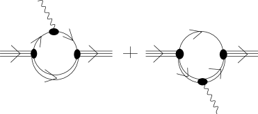
Figure 1: Feynman graphs for the evaluation of the nucleon electromagnetic current in the quark-diquark model. The double line represents the diquark t-matrix, the solid line the constituent quark propagator, and the black areas are the vertex functions and electromagnetic vertices.

Here $\Lambda_{Q}^{\mu}$ and $\Lambda_{D}^{\mu}$ are the electromagnetic vertices of the quark and the scalar diquark, both depending on the final and initial particle momenta. It is an easy task to use the Ward-Takahashi identities [23] for the quark and diquark vertices

$$q_{\mu}\left(S(\ell^{\prime})\Lambda_{Q}^{\mu}S(\ell)\right) = -Q_{Q}\left(S(\ell^{\prime})-S(\ell)\right)$$ (3.2)

$$q_{\mu}\left(\tau_{s}(\ell^{\prime})\Lambda_{D}^{\mu}\tau_{s}(\ell)\right) = iQ_{D}\left(\tau_{s}(\ell^{\prime})-\tau_{s}(\ell)\right)$$ (3.3)

to show the current and charge conservation for the nucleon:

$$q_{\mu}j_{N}^{\mu}(q) = Q_{N}\overline{\Gamma}_{N}(p^{\prime})\left(\Pi_{N}(p^{\prime})-\Pi_{N}(p)\right)\Gamma_{N}(p)=0$$ (3.4)

$$j^{\mu}(0) = Q_{N}\,\frac{p^{\mu}}{E_{Np}}\,,$$ (3.5)

where the electric charge of the nucleon $Q_{N}=Q_{Q}+Q_{D}$ is the sum of the quark and diquark electric charges.

The electromagnetic vertices in (3.1) describe the finite extension of the constituent quarks and the diquark. In general, they should be calculated off-shell consistently with the propagators $\tau_{s}$ and $S$, using Feynman diagrams or some ansatz which satisfies the Ward identities[8]. In the present work, however, our principal aim is to investigate the medium effects in a simple model calculation. For this purpose, we limit the complications caused by the quark and diquark sizes to a minimum, and use an on-shell (or pole) approximation for the quark and diquark currents appearing in Eq.(3.1):

$$\left(S(\ell^{\prime})\,\Lambda_{Q}^{\mu}\,S(\ell)\right) \longrightarrow Z_{Q}\left(S_{F}(\ell^{\prime})\,\hat{\Lambda}_{Q}^{\mu}\,S_{F}(\ell)\right)$$ (3.6)

$$\left(\tau_{s}(\ell^{\prime})\,\Lambda^{\mu}_{D}\,\tau_{s}(\ell)\right) \longrightarrow -g_{s}\left(\Delta_{Fs}(\ell^{\prime})\,\hat{\Lambda}_{D}^{\mu}\,\Delta_{Fs}(\ell)\right)\,,$$ (3.7)

where the on-shell (o.s.) vertices are denoted by a hat and given by the pole residues of the full quantities by

$$\hat{\Lambda}_{Q}^{\mu} \equiv Z_{Q}\left(\Lambda_{Q}^{\mu}\right)_{\rm o.s.}\equiv\gamma^{\mu}\,F_{1Q}(q^{2})+\frac{i\sigma^{\mu\nu}q_{\nu}}{2M}\,F_{2Q}(q^{2})$$ (3.8)

$$\hat{\Lambda}_{D}^{\mu} \equiv g_{s}\left(\Lambda_{D}^{\mu}\right)_{\rm o.s.}\equiv(\ell^{\prime}+\ell)^{\mu}\,F_{D}(q^{2}).$$ (3.9)

Here we introduced the quark and diquark form factors which satisfy $F_{1Q}(0)=Q_{Q},\,\,F_{D}(0)=Q_{D}$.

To understand (3.6) and (3.7), we note that in general the on-shell approximation for a vertex function $\Lambda^{\mu}(\ell^{\prime},\ell)$ can be formulated only if it appears between pole parts of Green functions, because only in this case one can approximate it by its value for on-shell momenta $\ell^{\prime},\,\ell$ . This is why in Eq.(3.6) and (3.7) we have replaced the propagators left and right to the vertex functions by their pole parts (see (2.11) and (2.12)), which is also essential in order to have charge conservation with the vertices (3.8) and (3.9).

We now can write down the form of the nucleon current (3.1) which will be used in the further calculations:

$$j_{N}^{\mu}(q)=\sqrt{\frac{M_{N}}{E_{Np}}\,\frac{M_{N}}{E_{Np^{\prime}}}}\,\overline{u}_{N}(p^{\prime})\left({\cal O}_{C}^{\mu}+{\cal O}_{Q}^{\mu}+{\cal O}_{D}^{\mu}\right)\,u_{N}(p)\,.$$ (3.10)

Here the first and second terms denote the contributions of the contact term and the pole term of the diquark t-matrix to the quark diagram (first diagram of Fig.1), and the third term is the contribution from the diquark diagram:

$${\cal O}_{C}^{\mu} = -\frac{4iG_{s}}{\hat{g}_{s}}\hat{Z}_{N}\int\frac{{\rm d}^{4}k}{(2\pi)^{4}}S_{F}(p^{\prime}-k)\left(\gamma^{\mu}F_{1Q}(q^{2})+\frac{i\sigma^{\mu\nu}q_{\nu}}{2M}F_{2Q}(q^{2})\right)S_{F}(p-k)$$

$${\cal O}_{Q}^{\mu} = i\hat{Z}_{N}\int\frac{{\rm d}^{4}k}{(2\pi)^{4}}S_{F}(p^{\prime}-k)\left(\gamma^{\mu}F_{1Q}(q^{2})+\frac{i\sigma^{\mu\nu}q_{\nu}}{2M}F_{2Q}(q^{2})\right)S_{F}(p-k)\Delta_{Fs}(k)$$

(3.12)

$${\cal O}_{D}^{\mu} = i\hat{Z}_{N}F_{D}(q^{2})\int\frac{{\rm d}^{4}k}{(2\pi)^{4}}\Delta_{Fs}(p^{\prime}-k)\left(p+p^{\prime}-2k\right)^{\mu}\Delta_{Fs}(p-k)\,S_{F}(k)\,.$$ (3.13)

(For the contact term, we replaced $G_{s}\rightarrow G_{s}/Z_{Q}^{2}$, so that $G_{s}$ in (LABEL:contact) is the renormalized coupling in the sense explained in Sect.2.) By using the elementary Ward-Takahashi identities $\mbox{$\!\not\!q$}=S_{F}^{-1}(\ell^{\prime})-S_{F}^{-1}(\ell)$ and $\ell^{\prime 2}-\ell^{2}=\Delta_{Fs}^{-1}(\ell^{\prime})-\Delta_{Fs}^{-1}(\ell)$ and the fact that on the nucleon mass shell $\Pi_{N}(p)=\Pi_{N}(p^{\prime})$, it is easy to check that the 3 parts in (3.10) satisfy current conservation separately. Similarly, charge conservation can be checked by using the elementary Ward identities $\gamma^{\mu}={\partial}S_{F}^{-1}(\ell)/\partial\ell^{\mu}$ and $2\ell^{\mu}=\partial\Delta_{Fs}^{-1}(\ell)/\partial\ell^{\mu}$, as well as $F_{1Q}(0)=Q_{Q}$, $F_{D}(0)=Q_{D}$. It has to be noted, however, the general Ward-Takahashi identity for an off-shell nucleon (the first equality in Eq.(3.4) without the nucleon spinor) is not valid in this approximation scheme.

It is not very difficult to evaluate the three loop integrals in (LABEL:contact)-(3.13), and in Appendix A the results are given in terms of the Dirac-Pauli form factors $F_{1N}$ and $F_{2N}$, which are defined by

$$j_{N}^{\mu} = \sqrt{\frac{M_{N}}{E_{Np}}\,\frac{M_{N}}{E_{Np^{\prime}}}}\,\overline{u}_{N}(p^{\prime})\left[\gamma^{\mu}F_{1N}(q^{2})+\frac{i\sigma^{\mu\nu}q_{\nu}}{2M_{N}}F_{2N}(q^{2})\right]u_{N}(p)\,.$$

In the following we will discuss various steps in the calculation of the nucleon form factors.

3.1 Naive quark-diquark model

The simplest approximation consists in assuming point couplings of the quarks and diquarks to the photon, i.e., replacing ${\displaystyle F_{1Q}\rightarrow Q_{Q}=\frac{1}{6}+\frac{\tau_{3}}{2}}$, ${\displaystyle F_{2Q}\rightarrow 0}$, ${\displaystyle F_{D}\rightarrow Q_{D}=\frac{1}{3}}$ in Eqs. (LABEL:contact)-(3.13). This approximation will be called the “naive quark-diquark model”, and the detailed expressions can be found in Appendix A.

3.2 Effects of finite diquark size

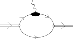
Figure 2: Graphical representation of the diquark form factor. The white circles denote the diquark vertex functions, and the black area is the quark electromagnetic vertex. (There is a second diagram where the photon couples to the other quark, but also an overall symmetry factor $\frac{1}{2}$.)

Here we consider the effect of the diquark form factor $F_{D}$, which has been defined in (3.9). The vertex $\Lambda^{\mu}_{D}$ is shown graphically in Fig.2, where the quark-diquark vertex functions are those appearing in the Lagrangian(2.3). We obtain

$$\hat{\Lambda}_{D}^{\mu}=i\,g_{s}\int\frac{{\rm d}^{4}k}{(2\pi)^{4}}\left\{{\rm Tr}\left[\gamma_{5}S(p^{\prime}+k)\Lambda_{Q}^{\mu}S(p+k)\gamma_{5}S(k)\right]\right\}\,,$$ (3.15)

where the trace refers to color, isospin and Dirac indices. Using the on-shell approximation (3.6), the definition of quark form factors (3.8), and also (2.12) and (LABEL:gs), we obtain

$$\hat{\Lambda}_{D}^{\mu} = 6i\,{\hat{g}}_{s}\int\frac{{\rm d}^{4}k}{(2\pi)^{4}}\left\{F_{1Q}^{(0)}(Q^{2}){\rm Tr}_{D}\left[\gamma_{5}S_{F}(p^{\prime}+k)\gamma^{\mu}S_{F}(p+k)\gamma_{5}S_{F}(k)\right]\right.$$ (3.16)

$$+ \left.F_{2Q}^{(0)}(Q^{2}){\rm Tr}_{D}\left[\gamma_{5}S_{F}(p^{\prime}+k)\frac{i\sigma^{\mu\nu}q_{\nu}}{2M}S_{F}(p+k)\gamma_{5}S_{F}(k)\right]\right\}\,.$$

Here $F_{1Q}^{(0)}$ and $F_{2Q}^{(0)}$ are the isoscalar parts of the quark form factors $F_{1Q}$ and $F_{2Q}$. The resulting diquark form factor $F_{D}$ is given in Appendix A.

3.3 Effects of meson cloud around constituent quarks

Here we consider the quark form factors arising from the pion cloud and vector mesons. For the pion cloud, we obtain from the definition (3.8) and the Feynman diagrams of Fig.3,

$$\hat{\Lambda}_{Q}^{\mu} = Z_{Q}\gamma^{\mu}Q_{Q}+Z_{Q}\int\frac{{\rm d}^{4}k}{(2\pi)^{4}}\left[-\gamma_{5}\tau_{i}\left(S(p^{\prime}-k)\Lambda_{Q0}^{\mu}S(p-k)\right)\tau_{i}\gamma_{5}\tau_{\pi}(k)\right.$$ (3.17)

$$+ \left.i\left(\tau_{\pi}(p^{\prime}-k)\Lambda_{\pi}^{\mu}\tau_{\pi}(p-k)\right)\gamma_{5}S(k)\gamma_{5}\right]\,.$$

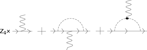
Figure 3: Pion cloud contributions to the quark electromagnetic vertex. $Z_{Q}$ is the quark wave function renormalization factor, and the dashed line represents the t-matrix in the pion channel. (This figure actually refers to the expression (LABEL:jq1), where the factor $Z_{Q}$ remains only for the “bare” term.)

Here $\tau_{\pi}$ is the reduced $q{\overline{q}}$ t-matrix is the pion channel, which can be approximated in the same way as the diquark t-matrix (2.11):

$$\tau_{\pi}(k) = \frac{-2iG_{\pi}}{1+2G_{\pi}\Pi_{\pi}(k^{2})}\longrightarrow-2iG_{\pi}+\frac{ig_{\pi}}{k^{2}-M_{\pi}^{2}}\equiv-2iG_{\pi}+ig_{\pi}\Delta_{F\pi}(k)\,.$$

(3.18)

The bubble graph in the pion channel is $\Pi_{\pi}=\Pi_{s}$ (see (2.5)), and the residue $g_{\pi}$ will be given in Eq.(3.24) below.

The expression (3.17) is formally similar to the nucleon current (3.1). The presence of the first term simply expresses the fact that in the NJL model the (bare) quarks are present from the beginning, and the factor $Z_{Q}$ gives the probability of having a constituent quark without its pion cloud. It has been expressed in Eq.(2.12) in terms of the self energy

$$\Sigma_{Q}(p)=-3\int\frac{{\rm d}^{4}k}{(2\pi)^{4}}\left(\gamma_{5}S(p-k)\gamma_{5}\right)\tau_{\pi}(k)\,.$$ (3.19)

The quark electromagnetic vertex ${\Lambda}_{Q0}^{\mu}$ in (3.17) will be approximated by its point form after processing the renormalization factor $Z_{Q}$, and the pion electromagnetic vertex $\Lambda_{\pi}^{\mu}\equiv\tau_{i}\Lambda_{\pi,ij}^{\mu}\tau_{j}$ is similar to the diquark vertex of Fig.2, but with point quark-photon couplings, as will be specified below.

We now follow the same steps as for the calculation of the nucleon current: We use the on-shell approximation for the quark and pion vertices

$$\left(S(\ell^{\prime})\,\Lambda_{Q0}^{\mu}\,S(\ell)\right) \longrightarrow Z_{Q}\left(S_{F}(\ell^{\prime})\,\hat{\Lambda}_{Q0}^{\mu}\,S_{F}(\ell)\right)$$ (3.20)

$$\left(\tau_{\pi}(\ell^{\prime})\,\Lambda^{\mu}_{\pi}\,\tau_{\pi}(\ell)\right) \longrightarrow -g_{\pi}\left(\Delta_{F\pi}(\ell^{\prime})\hat{\Lambda}_{\pi}^{\mu}\,\Delta_{F\pi}(\ell)\right)\,,$$ (3.21)

where the on-shell vertices are defined by

$$\hat{\Lambda}_{Q0}^{\mu} \equiv Z_{Q}\left(\Lambda_{Q0}^{\mu}\right)_{\rm o.s.}\equiv\gamma^{\mu}\,Q_{Q}$$ (3.22)

$$\hat{\Lambda}_{\pi,ij}^{\mu} \equiv g_{\pi}\left(\Lambda_{\pi,ij}^{\mu}\right)_{\rm o.s.}\equiv(\ell^{\prime}+\ell)^{\mu}\left(-i\epsilon_{ij3}\right)F_{\pi}(q^{2})\,.$$ (3.23)

Using $S(k)=Z_{Q}S_{F}(k)$ in the expression for $\Pi_{\pi}$, we get

$$g_{\pi}^{-1}=\left(-\frac{\partial\Pi_{\pi}(q)}{\partial q^{2}}\right)_{q^{2}=M_{\pi}^{2}}=Z_{Q}^{2}\,\left(-\frac{\partial\hat{\Pi}_{\pi}(q)}{\partial q^{2}}\right)_{q^{2}=M_{\pi}^{2}}\equiv Z_{Q}^{2}\,\hat{g}_{\pi}^{-1}\,,$$ (3.24)

with the renormalized bubble graph $\hat{\Pi}_{\pi}=\hat{\Pi}_{s}$, see (2.15). Then Eq. (3.17) becomes

$$\hat{\Lambda}_{Q}^{\mu} = Z_{Q}\gamma^{\mu}Q_{Q}-i\hat{g}_{\pi}\frac{1}{2}(1-\tau_{3})\int\frac{{\rm d}^{4}k}{(2\pi)^{4}}\gamma_{5}\left(S_{F}(p^{\prime}-k)\gamma^{\mu}S_{F}(p-k)\right)\gamma_{5}\Delta_{F\pi}(k)$$

$$- 2i\,\tau_{3}\,\hat{g}_{\pi}\,F_{\pi}(q^{2})\int\frac{{\rm d}^{4}k}{(2\pi)^{4}}\left(\Delta_{F\pi}(p^{\prime}-k)\left(p^{\prime}+p-2k\right)^{\mu}\Delta_{F\pi}(p-k)\right)\gamma_{5}S_{F}(k)\gamma_{5}\,.$$

Here we note that the contribution of the contact term ($2iG_{\pi}$) to the quark diagram has been dropped in order to avoid double counting: Because we always assume that our interaction Lagrangians are Fierz symmetric, it is easy to see that this contribution can be incorporated into the vector meson channel, which will be separately considered below. By using $S=Z_{Q}S_{F}$ in the self energy (3.19) and in the expression for $Z_{Q}$ of Eq.(2.12), we see that

$$Z_{Q}=1+\left(\frac{\partial\hat{\Sigma}_{Q}}{\partial\mbox{$\!\not\!p$}}\right)_{\mbox{$\!\not\!p$}=M}\,,$$ (3.26)

where the renormalized quark self energy is given by

$$\hat{\Sigma}_{Q}(p)=-3i\hat{g}_{\pi}\int\frac{{\rm d}^{4}k}{(2\pi)^{4}}\left(\gamma_{5}S_{F}(p-k)\gamma_{5}\right)\Delta_{F\pi}(k)\,.$$ (3.27)

The further evaluation of the loop integral (LABEL:jq1) is left to Appendix B, where the contributions to the quark form factors $F_{1Q}$ and $F_{2Q}$ are given. The pion electromagnetic vertex is evaluated from the definition (3.23) and a Feynman diagram similar to Fig.2 for an external pion, but with a point quark-photon coupling:

$$\hat{\Lambda}^{\mu}_{ij}=\left(-i\,\epsilon_{ij3}\right)\,6i\,\hat{g}_{\pi}\int\frac{{\rm d}^{4}k}{(2\pi)^{4}}{\rm Tr}_{D}\left[\gamma_{5}S_{F}(p^{\prime}+k)\gamma^{\mu}S_{F}(p+k)\gamma_{5}S_{F}(k)\right]\,.$$ (3.28)

The explicit form of $F_{\pi}(q^{2})$ is given in Appendix B.

Finally, we consider the corrections of the quark electromagnetic vertex arising from vector mesons, similar to vector meson dominance (VMD) models. If our original interaction Lagrangian contains terms of the form

$${\cal L}_{I,v}=-G_{\omega}\left(\overline{\psi}\gamma^{\mu}\psi\right)^{2}-G_{\rho}\left(\overline{\psi}\gamma^{\mu}{\mbox{\boldmath${\tau}$}}\psi\right)^{2}\,,$$ (3.29)

then the point-like quark-photon vertices in the diagrams of Fig.3 and the pion vertex $\Lambda_{\pi}^{\mu}$ are replaced by the VMD vertex shown in Fig.4.

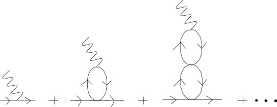
Figure 4: The corrections to the quark electromagnetic vertex arising from vector meson dominance. Here the 4-fermi interactions refer to the vector channel (see Eq.(3.29)), i.e., terms with tensor coupling to the external quark are not included.

Because of the transverse structure of the bubble graphs in the vector channel, this leads to the following renormalization:

$$\gamma^{\mu}Q_{Q} \longrightarrow \frac{1}{6}\left[\gamma^{\mu}-\frac{2G_{\omega}\hat{\Pi}_{V}(q^{2})}{1+2G_{\omega}\hat{\Pi}_{V}(q^{2})}\left(\gamma^{\mu}-\frac{q^{\mu}\mbox{$\!\not\!q$}}{q^{2}}\right)\right]$$ (3.30)

$$+ \frac{\tau_{3}}{2}\left[\gamma^{\mu}-\frac{2G_{\rho}\hat{\Pi}_{V}(q^{2})}{1+2G_{\rho}\hat{\Pi}_{V}(q^{2})}\left(\gamma^{\mu}-\frac{q^{\mu}\mbox{$\!\not\!q$}}{q^{2}}\right)\right]\,,$$ (3.31)

where the form of $\hat{\Pi}_{V}$ is given in Appendix B. Because our quark-photon vertex in (3.8) is defined for on-shell quarks, the terms ${\displaystyle\propto\frac{q^{\mu}\mbox{$\!\not\!q$}}{q^{2}}}$ do not contribute. Therefore the isoscalar (or isovector) parts in the quark electromagnetic vertex should be multiplied by a form factor $F_{\omega}(q^{2})$ (or $F_{\rho}(q^{2})$), where

$$F_{\alpha}(q^{2})=\frac{1}{1+2G_{\alpha}\hat{\Pi}_{V}(q^{2})}\,\,\,\,\,\,\,(\alpha=\omega,\rho)\,.$$ (3.32)

4 Results for the nucleon form factors

In this section we will show our results for the nucleon form factors. First we discuss our model parameters and particle masses. The parameters are the same as in Refs.[11, 15]: The IR cut-off $\Lambda_{\rm IR}$ is fixed as $0.2$ GeV, the constituent quark mass at zero nucleon density is $M_{0}=0.4$ GeV, and $G_{\pi}$, $\Lambda_{\rm UV}$ are determined so as to reproduce $M_{\pi}=0.14$ GeV and $f_{\pi}=93$ MeV. This gives $G_{\pi}=19.60$ GeV^-2 and $\Lambda_{\rm UV}=0.6385$ GeV. The coupling constant $G_{s}$ is determined so as to reproduce $M_{N0}=0.94$ GeV, which gives the ratio $G_{s}/G_{\pi}=0.508$. The coupling constant $G_{\omega}$ is determined so that the curve for the NM binding energy per nucleon $(E_{B}/A$) as a function of the density passes through the empirical saturation point ($\rho,E_{B}/A)=(0.16$ fm${}^{-3},\,15$ MeV), which gives the ratio $G_{\omega}/G_{\pi}=0.37$. Finally, for the VMD form factors (3.32) we also need the coupling constant $G_{\rho}$, which is determined by reproducing the empirical symmetry energy coefficient $a_{4}=35$ MeV at the density $\rho=0.16$ fm^-3, which gives $G_{\rho}/G_{\pi}=0.091$

In Table 1 we list the effective quark, diquark, nucleon and pion masses for the densities $\rho=0,\,0.08,\,0.16,$ and $0.24$ fm^-3. Concerning the pion mass in the medium, we use a general result based on chiral symmetry [25], which for the NJL model implies that the product $M_{\pi}^{2}\,\cdot M$ is a constant independent of density, see Eq.(2.58) of Ref.[11]. We therefore use $M_{\pi}^{2}=M_{\pi 0}^{2}\cdot M_{0}/M$. Also listed in Table 1 are the values of $\hat{g}_{s}$, $\hat{g}_{\pi}$, $\hat{Z}_{N}$ and $Z_{Q}$.

	$\rho=0$	$\rho=0.08\,$fm-3	$\rho=0.16\,$fm-3	$\rho=0.24\,$fm-3
$M$	0.4	0.353	0.308	0.268
$M_{s}$	0.576	0.493	0.413	0.342
$M_{N}$	0.94	0.818	0.707	0.619
$M_{\pi}$	0.14	0.149	0.159	0.171
$\hat{g}_{s}$	18.26	17.17	16.20	15.40
$\hat{g}_{\pi}$	17.81	14.29	11.60	9.70
$\hat{Z}_{N}$	44.32	47.62	50.38	51.97
$Z_{Q}$	0.808	0.832	0.852	0.869

Table 1: Effective masses for the quark, the diquark, the nucleon and the pion (all in GeV), and pole residues $\hat{g}_{s}$, $\hat{g}_{\pi}$, $\hat{Z}_{N}$ and $Z_{Q}$ for four values of the density.

We will discuss our results for the nucleon form factor in terms of the Dirac-Pauli form factors defined by Eq.(LABEL:par1). In the discussion of medium effects, in particular the effects of the reduced nucleon mass ($M_{N}<M_{N0}$), we will also refer to an equivalent parametrization in terms of the “orbital form factor” $G_{L}$ and the “spin form factor” $G_{S}$:

$$j_{N}^{\mu} = \sqrt{\frac{M_{N}}{E_{Np}}\,\frac{M_{N}}{E_{Np^{\prime}}}}\,\overline{u}_{N}(p^{\prime})\left[\frac{\left(p^{\prime}+p\right)^{\mu}}{2M_{N0}}G_{L}(q^{2})+\frac{i\sigma^{\mu\nu}q_{\nu}}{2M_{N0}}G_{S}(q^{2})\right]u_{N}(p)$$

The relations to the Dirac-Pauli form factors are

$$G_{L}=\frac{M_{N0}}{M_{N}}F_{1N}\,,\,\,\,\,\,\,\,\,\,\,G_{S}=\frac{M_{N0}}{M_{N}}(F_{1N}+F_{2N})\,.$$ (4.2)

We introduce these form factors here, because $F_{1}$ and $F_{2}$ do not directly reflect the enhancement of the nucleon orbital current (${\mbox{\boldmath${j}$}}_{\rm N,orb}$) arising from the reduced nucleon mass (enhanced nuclear magneton) . Moreover, the parametrization (LABEL:par2) for the space part of the current has more connection to the traditional calculations of nuclear magnetic properties [28], because the values of these form factors at $q=0$ reduce to the orbital and spin g-factors: $g_{L}=G_{L}(0)$, $g_{S}=G_{S}(0)$.

Here we would like to point out that these different ways to discuss the medium modifications of the nucleon current remind us that the form factors of a nucleon in the medium are not directly observable quantities: Ultimately the current $j_{N}^{\mu}$ has to be used in a nuclear structure calculation of observable cross sections. Our current $j_{N}^{\mu}$ reflects only those effects which are not taken into account in nuclear structure calculations, i.e., the effects of the nuclear mean fields on the internal motion of quarks in the nucleon. Other effects, which explicitly depend on the density and have their origin in the Pauli principle on the level of nucleons, must be considered in the nuclear part of the calculation . As an example of such a calculation for the case of nuclear matter, we will consider the response function for quasielastic electron scattering in Sect.5.

For the zero density (single nucleon) case, it is possible to define a Breit frame where $q_{0}=0$, and in this frame the nucleon current can be expressed in terms of the familiar electric and magnetic form factors

$$G_{E}(q^{2}) = F_{1}(q^{2})+\frac{q^{2}}{4M_{N}^{2}}F_{2}(q^{2})$$ (4.3)

$$G_{M}(q^{2}) = F_{1}(q^{2})+F_{2}(q^{2})\,.$$ (4.4)

We will compare our calculated form factors for zero density with the empirical dipole form factors, defined by

$$G_{Ep} = G_{Mp}/\mu_{p}=G_{Mn}/\mu_{n}=\frac{1}{\left(1-q^{2}/0.71\,{\rm GeV}^{2}\right)^{2}}$$

$$F_{1n} = 0\,.$$ (4.5)

For a nucleon moving in the medium, however, one cannot define a Breit frame, and consequently the combinations (4.3) and (4.4) do not enter naturally in the expressions for nuclear observables, like response functions or elastic form factors. For the finite density case we will therefore discuss our results in terms of the form factors $F_{1}$ and $F_{2}$, or $G_{L}$ and $G_{S}$.

The results for the form factors at zero density (free nucleon case) are shown in Figs.5-8. There we plot (i) the results of the naive quark-diquark model (see Sect.3.1) without (dotted lines) and with (dashed lines) the contact term contribution to the quark diagram of Fig.1, (ii) the results obtained by including in addition the effects of the diquark form factor (dash-dotted lines), and (iii) the total result including also the pion and VMD effects.

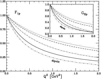
Figure 5: The form factor $F_{1p}$ for zero density. The dotted line is the result of the naive quark-diquark model without the contact term, to which the other contributions are successively added as follows: Dashed line: including contact term; dash-dotted line: including diquark form factor; solid line: full results including pion and vector meson contributions. The dash-double dotted line labeled “dipole” shows the dipole parametrization. The insert shows the form factor $G_{Ep}$, with the same meaning of the lines.

Fig. 5 shows that in the naive quark-diquark model the electric size of the proton is too small and the form factors $F_{1p}$ and $G_{Ep}$ fall off too slowly. The situation improves when the diquark form factor is included, and also the pion cloud gives some positive contribution to the electric size of the proton . The total result for $F_{1p}$ still lies above the empirical dipole form factor, but we can expect that the further inclusion of axial vector diquarks and pion cloud effects around the nucleon will lead to a satisfactory description.

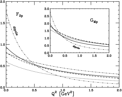
Figure 6: Same as Fig. 5 for the form factors $F_{2p}$ (main part) and $G_{Mp}$ (insert) for zero density.

Fig. 6 shows that the proton magnetic moment in the naive quark-diquark picture is too small, which is expected and also well known[17, 24]. The finite size effects of the scalar diquark do not contribute much in this case. The inclusion of the contact term in the quark diagram of Fig.1 improves the situation somewhat. By using a Fierz transformation, this term is actually seen to be equivalent to a vector meson contribution (like shown in Fig.4 for the quark), but with a tensor coupling ($\propto\sigma^{\mu\nu}q_{\nu}$) to the nucleon. Also the pion cloud, which leads to anomalous magnetic moments of the constituent up and down quarks, gives a positive contribution to the proton magnetic moment, but the total result is still too small. It is, however, known that the axial vector diquark and the pion cloud around the nucleon give large contributions to the magnetic moment and the associated form factors, and Fig.6 shows how far one can go in the simple quark - scalar diquark description.

The importance of the diquark form factor is also seen for the neutron form factors $F_{1n}$ and $G_{En}$, which are shown in Fig. 7. The naive quark-diquark model gives an electric form factor which is too large in comparison to the experimental one (note that the experimental $G_{En}$ is smaller than the “dipole form factor” shown in Fig. 7), and the diquark form factor, which suppresses the (positive) contribution from the second diagram of Fig.1 relative to the (negative) first one, is essential to obtain reasonable values. The electric size of the neutron is somewhat too small in magnitude, but this is because the absolute value of the magnetic moment is too small . In this connection, it is interesting to observe that the result for $F_{1n}$, and in particular its contribution to the electric radius, is very small, and therefore the electric size of the neutron is almost entirely due to the “Foldy term” [26].

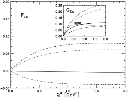
Figure 7: Same as Fig. 5 for the form factors $F_{1n}$ (main part) and $G_{En}$ (insert) for zero density. The dipole parametrization of $F_{1n}$ is zero by definition and therefore not indicated here.

The situation for the form factors $F_{2n}$ and $G_{Mn}$ shown in Fig. 8 is similar to the case of the proton (Fig. 6), i.e., the contact term and the pion cloud around the constituent quarks give some improvements of the magnetic moment, but the total result is still too small. This, and the fact that the form factors fall off too slowly, again points out the necessity to include the axial vector diquark channel.

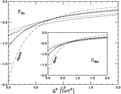
Figure 8: Same as Fig. 5 for the form factors $F_{2n}$ (main part) and $G_{Mn}$ (insert) for zero density.

The medium modifications of the nucleon form factors are shown in Figs. 9-12, where we plot the results for $\rho=0$ (dotted lines), $\rho=0.08$ fm^-3 (dashed lines), $\rho=0.16$ fm^-3 (solid lines), and $\rho=0.24$ fm^-3 (dash-dotted lines).

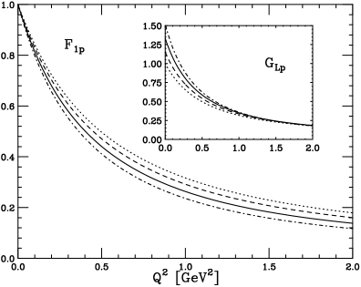
Figure 9: The form factor $F_{1p}$ for the cases $\rho=0$ (dotted line), $\rho=0.08$ fm^-3 (dashed line), $\rho=0.16$ fm^-3 (solid line), $\rho=0.24$ fm^-3 (dash-dotted line). The insert shows the proton orbital form factor $G_{Lp}$ defined in Eq.(LABEL:par2) with the same meaning of the lines.

The result for $F_{1p}$ of Fig. 9 indicates that the electric size of the proton in the medium is somewhat enhanced. The orbital form factor $G_{Lp}$ shown in the insert of Fig.9 demonstrates the enhancement of the orbital current (${\mbox{\boldmath${j}$}}_{\rm N,orb}$) due to the reduced effective nucleon mass, see Eq.(4.2). We have to remind, however, that the isoscalar part of this enhancement is in a sense spurious, because in an actual nuclear calculation it is canceled by the “backflow” effect[27], which in our language arises from Z-graphs, i.e., the Pauli blocking part of the $N\overline{N}$ excitation piece (see the detailed discussions in Ref.[28, 29] on the backflow in relativistic meson-nucleon theories). Namely, the proton orbital g-factor, which is roughly $M_{N0}/M_{N}$ in a Hartree calculation, becomes approximately $\frac{1}{2}(1+M_{N0}/M_{N})$ after the inclusion of the backflow, where the first term is the isoscalar and the second one the isovector piece.

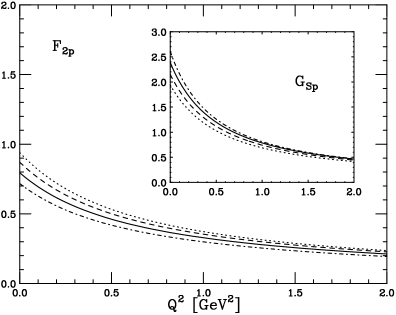
Figure 10: Same as Fig.9 for the form factor $F_{2p}$ (main part) and the proton spin form factor $G_{Sp}$ defined in Eq.(LABEL:par2) (insert).

Fig. 10 shows that the medium effects tend to decrease the “intrinsic” anomalous magnetic moment of the proton, but when combined with the enhancement of the nuclear magneton, the spin g-factor is enhanced, as shown in the insert of Fig.10. It is interesting that a very similar result has been obtained also in hadronic models[18]. Therefore, the quark effects considered here do not lead to a quenching of the spin g-factor, as would be desirable to explain the missing quenching of isovector nuclear magnetic moments [28], but rather to an enhancement . The figure also shows that the magnetic size of the proton becomes somewhat larger in the medium.

The results for the neutron form factor $F_{1n}$ in Fig. 11 show that the effect of finite diquark size, which was very important for the zero density case (Fig.7) to reduce $F_{1n}$ to reasonable values, increases with increasing density. That is, the diquark form factor at finite density further suppresses the positive contribution of the diquark diagram in Fig.1. The orbital form factor $G_{Ln}$ shown in the insert of Fig.11 again demonstrates the enhancement of the nuclear magneton, but we have to keep in mind that the backflow effect will change the neutron orbital g-factor from the present value $0$ to roughly $\frac{1}{2}\left(1-M_{N0}/M_{N}\right)<0$, and that effects of the pion cloud around the nucleon are known to further enhance the magnitude of the neutron orbital g-factor.

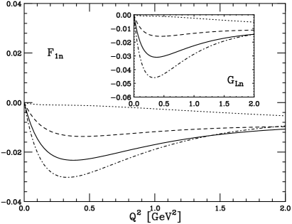
Figure 11: Same as Fig.9 for the form factor $F_{1n}$ (main part) and the neutron orbital form factor $G_{Ln}$ defined in Eq.(LABEL:par2) (insert).

The medium effects on the neutron form factor $F_{2n}$ shown in Fig.12 are qualitatively similar to the proton case of Fig.10: They decrease the absolute value of the “intrinsic” anomalous magnetic moment of the neutron, but when combined with the enhancement of the nuclear magneton the neutron spin g-factor becomes slightly enhanced in magnitude, as shown in the insert of Fig.12. The magnetic size of the neutron is not changed much, and the total medium effects on the neutron spin form factor are very small.

An interesting common feature of the results shown in Fig. 9-12 is that the medium modifications of the orbital and spin form factors ($G_{L}(Q^{2})$ and $G_{S}(Q^{2})$) always decrease with increasing $Q^{2}$. This is consistent with the intuitive expectation that the internal structure of the nucleon at short distances is not influenced much by the mean nuclear fields, and again indicates that these form factors reflect the change of the nucleon current in the medium more directly and transparently than the form factors $F_{1}$, $F_{2}$ themselves, or any other combination of them.

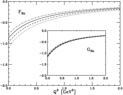
Figure 12: Same as Fig.9 for the form factor $F_{2n}$ (main part) and the neutron spin form factor $G_{Sn}$ defined in Eq.(LABEL:par2) (insert).

5 Application: The longitudinal nuclear response function

As an application of the medium effects discussed in the previous section to the calculation of nuclear quantities, we consider the longitudinal response function for quasielastic electron scattering. Generally, quasielastic processes are the ideal places to investigate medium modifications of nucleon form factors, because the on-shell kinematics, which is used in the derivation of the nucleon form factors, is justified. Recently, experiments on the polarization transfer in proton knock-out reactions have been carried out in the region of quasielastic kinematics at large momentum transfers[5], and the results were discussed in connection to the predicted medium modifications of nucleon form factors[6]. In this work, however, we will consider the simpler case of the inclusive quasielastic response function in the region of lower momentum transfers. In previous works[31], based on purely hadronic models, it was shown that this quantity is quite sensitive to medium modifications of form factors, and here we wish to apply our more microscopic quark description to the longitudinal response function in nuclear matter.

The longitudinal response function in isospin symmetric nuclear matter is expressed as

$$S_{L}(\omega,{\mbox{\boldmath${q}$}})=\frac{2Z}{\pi\rho}\,{\rm Im}\,\Pi_{L}(\omega,{\mbox{\boldmath${q}$}})\,,$$ (5.1)

where $\Pi_{L}(\omega,{\mbox{\boldmath${q}$}})$ is the 2-point (correlation) function for two external operators $j_{N}^{0}$. In the mean field (Hartree) approximation, this is expressed by the first diagram of Fig.13, and if we include the direct terms of the NN interaction in the ladder approximation, this gives the familiar RPA series.

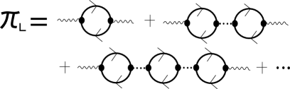
Figure 13: Graphical representation of the longitudinal current-current correlation function. The solid lines represent nucleons, and the dashed lines the interaction between nucleons. The external operator is $j_{N}^{0}$. The first diagram gives the Hartree response function, and the others the RPA corrections.

The relativistic calculation of $\Pi_{L}$ follows the lines given in Ref.[32, 33], i.e., the bubble graphs in Fig.13 consist of the nucleon particle- nucleon hole excitations and the Pauli blocking part of the nucleon particle- antinucleon excitations (Z-graphs). The other effects, which are not taken into account explicitly in Fig.13, are summarized in the density dependent electromagnetic vertices. Previous calculations based on hadronic models[31] incorporated the vacuum fluctuations on the level of nucleons (that is, the change of the nucleon-antinucleon vacuum polarization graphs in the presence of the nuclear mean fields), but it is more appropriate to describe these vacuum fluctuations on the level of quarks . Therefore we use our nucleon current (3.1) for $\mu=0$ at the electromagnetic vertices of Fig.13.

For the RPA calculation, we need the NN interaction kernel in our effective quark theory, which is shown graphically in Fig.14 and expressed as

$$V_{NN}(k)\equiv V_{\sigma}(k)\,({\mbox{\boldmath${1}$}})_{1}\cdot({\mbox{\boldmath${1}$}})_{2}+V_{\omega}(k)\,(\gamma_{\mu})_{1}\cdot({\gamma^{\mu}})_{2}$$ (5.3)

$$=\frac{-2G_{\pi}}{1-2G_{\pi}\,\hat{\Pi}_{\sigma}(k^{2})+2G_{\pi}\,\delta M_{s}^{2}}\left(\frac{{\rm d}M_{N}}{{\rm d}M}\right)^{2}F_{\sigma}^{2}(k^{2})\,({\mbox{\boldmath${1}$}})_{1}\cdot({\mbox{\boldmath${1}$}})_{2}$$

$$+ \frac{2G_{\omega}}{1+2G_{\omega}\,\hat{\Pi}_{V}(k^{2})}\,9\,F_{\omega}^{2}(k^{2})\,(\gamma_{\mu})_{1}\cdot({\gamma^{\mu}})_{2}$$ (5.4)

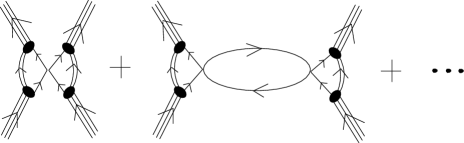
Figure 14: The NN interaction of Eq.(5.3) in the present quark-diquark model. Only those terms arising from the interaction of the two spectator quarks are shown, there are also equivalent graphs from the interaction between the quarks inside the diquarks. The term $\delta M_{\sigma}^{2}$, which is included in Eq.(5.3), is not shown explicitly in this figure.

Here the first factor in (5.3) is the reduced $q{\overline{q}}$ t-matrix in the sigma meson channel, and the corresponding bubble graph $\hat{\Pi}_{\sigma}$ is given in Appendix C. The derivation of the effective NN interaction in the NJL model[11], however, has shown that in addition to the part $\hat{\Pi}_{\sigma}$, which describes the $q\overline{q}$ exchange (see Fig.14), there is also a nuclear part which consists of (i) the Z-graph, and (ii) a contact term arising from an induced $\overline{N}\sigma^{2}N$ interaction. Concerning the Z-graph, we note that this is just the Pauli blocking part to the $N\overline{N}$ bubble graph, which is taken into account explicitly in the RPA series of Fig.13 and therefore should not be included in the interaction. (Numerically the Z-graph contribution is small compared to $\hat{\Pi}_{\sigma}$ because of the reduced $\sigma$N coupling in the medium, see Ref.[11].) The self energy correction for the sigma meson arising from the induced $\overline{N}\sigma^{2}N$ contact interaction is included in (5.3) as the density-dependent constant[11]

$$\delta M_{\sigma}^{2}=4\left(\frac{{\rm d}^{2}M_{N}}{{\rm d}M^{2}}\right)\int\frac{{\rm d}^{3}k}{(2\pi)^{3}}\frac{M_{N}}{E_{N}(k)}\Theta(p_{F}-|{\mbox{\boldmath${k}$}}|)\,.$$ (5.5)

The $NN\sigma$ coupling constant at zero momentum is proportional to ${\rm d}M_{N}/{\rm d}M$, and its square appears in (5.3). The $NN\sigma$ vertex form factor $F_{\sigma}(k^{2})$ is normalized to $F_{\sigma}(0)=1$. The first factor in (5.4) is the reduced $q{\overline{q}}$ t-matrix in the $\omega$-meson channel, and the corresponding bubble graph $\hat{\Pi}_{V}$ is the same as in the VMD correction to the quark form factors (Fig.4). The $NN\omega$ coupling constant at zero momentum is proportional to the number of quarks in the nucleon, and the vertex form factor $F_{\omega}(k^{2})$ is normalized as $F_{\omega}(0)=1$.

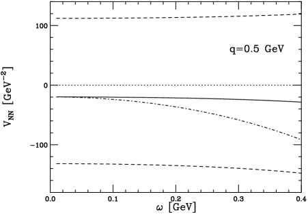
Figure 15: The NN interaction for $|{\mbox{\boldmath${q}$}}|=0.5$ GeV as a function of $\omega$. The lower dashed line shows the attractive part $V_{\sigma}$ of Eq.(5.3), the upper dashed line the repulsive piece $V_{\omega}$ of Eq.(5.4), the solid line shows their naive sum, and the dash-dotted line shows the combination $V_{\sigma}+V_{\omega}(1-\omega^{2}/|{\mbox{\boldmath${q}$}}|^{2})$.

By taking matrix elements of (5.3), (5.4) between the nucleon spinors, it is easy to see that for $k=0$ and for nucleons at the Fermi surface we just get the Landau-Migdal interaction derived more generally in Ref.([11]) (except for the Z-graph contributions as explained above). The form factor $F_{\omega}$ is equal to $(F_{1p}+F_{1n})$, which was calculated in the previous sections. The scalar form factor $F_{\sigma}$ should in principle be calculated independently from the Feynman diagrams of Fig.1 by using the external operator ${1}$. However, because the calculations discussed below show that the RPA effects are numerically not very important, we will simply assume the same form factor as for the $NN\omega$ coupling ($F_{\sigma}=F_{\omega}$).

The two parts of the NN interaction, $V_{\sigma}$ of (5.3) and $V_{\omega}$ of (5.4) , are shown by the lower and upper dashed lines, respectively, in Fig.15 for the kinematics needed in the calculation of the response function, $|{\mbox{\boldmath${q}$}}|=0.5$ GeV and $0<\omega<0.4$ GeV. As in the case of relativistic hadronic models[34], we see large cancellations between the attractive scalar and repulsive vector parts. The solid line shows the naive sum of the two dashed lines, while the dash-dotted line shows the combination $V_{\sigma}+V_{\omega}(1-\omega^{2}/|{\mbox{\boldmath${q}$}}|^{2})$, which includes the effect of the longitudinal space component of the $\omega$ exchange and is more relevant for the longitudinal response function [31]. The results shown in Fig. 15 can be reproduced almost exactly by an approximate form in terms of Yukawa potentials, if the coupling constants and meson masses are defined at $k^{2}=0$. This is discussed in Appendix C, where also numerical values are given.

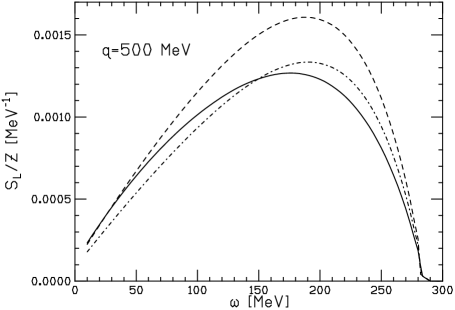
Figure 16: The longitudinal response function calculated in nuclear matter for density $\rho=0.16$ fm^-3 and $|{\mbox{\boldmath${q}$}}|=500$ MeV as a function of $\omega$. Dashed line: Hartree response with free dipole form factors, dash-dotted line: Hartree response including the medium corrections to the nucleon form factors, solid line: RPA response including the medium corrections to the nucleon form factors. The NN interaction used for the RPA calculation is the one shown in Fig.15, but multiplied by meson-nucleon form factors including medium corrections as explained in the main text.

The result for the longitudinal response function of NM ($\rho=0.16$ fm^-3) for $|{\mbox{\boldmath${q}$}}|=0.5$ GeV is shown in Fig. 16. The dashed line is the Hartree response with the free dipole form factors, and the dash-dotted line is obtained by adding our calculated medium corrections $\Delta F(q^{2};\rho)=F(q^{2},\rho)-F(q^{2},\rho=0)$ to the free dipole form factors. (Here $F$ denotes any of the Dirac-Pauli form factors.) We see that, even in this region of relatively low momentum transfers, the medium effects are appreciable. Finally, the solid line shows the result obtained by further adding the RPA corrections with the NN interaction derived above and using the density dependent meson-nucleon form factors.

We do not show a comparison to experimental data in Fig.16 because of two reasons: First, our calculation refers to NM and cannot be applied directly to finite nuclei, although for the case of ⁴⁰Ca the results are qualitatively very similar to the NM results, see Ref.[31]. Second, the analysis of the experimental data is still controversial, mainly because of the model dependence of the Coulomb corrections[35, 4, 36] .

6 Summary

In this paper we used a simple quark-scalar diquark picture for the single nucleon to describe the electromagnetic form factors of a nucleon bound in the nuclear medium. We used the nuclear matter equation of state derived within the same effective quark theory to assess the effect of the mean nuclear fields on the internal quark structure and the form factors of a bound nucleon, taking into account also the meson cloud around the constituent quarks. We have shown that this simple model gives reasonable results for the Dirac form factors of the free nucleon if the finite size of the diquark is taken into account. This is particularly important for the neutron in order to obtain a small $F_{1}$, consistent with observations. Concerning the Pauli form factors, in particular the anomalous magnetic moments and the behavior for large $Q^{2}$, one would need to further add the effect of the axial vector diquark and its finite size to achieve a reasonable description.

The medium modifications of the form factors associated with the orbital current are significant in the region of low and intermediate $Q^{2}$, and partially associated with an increase of the electric size in the medium. The form factors associated with the spin current are enhanced because of the reduced nucleon mass, but due to a simultaneous decrease of the intrinsic anomalous magnetic moment, the total changes are not very large; in particular for the neutron they are almost zero. For both kinds of form factors - orbital and spin -, the medium modifications decrease with increasing $Q^{2}$. This is consistent with the intuitive expectation that the mean fields, which reflect the long range nuclear correlations, should not influence the structure of the nucleon at short distances.

As an application, we considered the longitudinal response function of nuclear matter for inclusive quasielastic electron scattering. Even in this region of relatively low momentum transfer, the medium effects on the nucleon form factors give rise to an appreciable quenching of the response function. In order to take into account the RPA-type correlations between the nucleons, we derived the NN interaction in the present quark model for the isoscalar channel, which is most important for the longitudinal response function. In the limit of zero momentum transfer (Landau limit), this interaction agrees with the more general Landau-Migdal effective interaction, which was derived in earlier works for this particular quark theory, and has many features which are similar to relativistic meson-nucleon theories. In particular, it is on the average repulsive in the region below the quasielastic peak, and becomes attractive for higher energy transfers.

We finally would like to remark that the language of effective quark theories is very appropriate to address the problem of medium modifications of nucleon properties. This work represents one further step toward the goal of describing relativistic nuclear systems by taking into account the quark substructure of the constituent hadrons.

Acknowledgment

W.B. wishes to thank A.W. Thomas for many helpful discussions. This work was supported by the Grant in Aid for Scientific Research of the Japanese Ministry of Education, Culture, Sports, Science and Technology, Project No. C-16540267.

Appendices

Appendix A Expressions for the nucleon form factors

Here we give the explicit expressions for the contributions of the 3 terms in Eq.(LABEL:contact)-(3.13) to the nucleon Dirac-Pauli form factors defined in (LABEL:par1). They can be derived by invariant integration in the usual way, i.e., by (i) introducing Feynman parameters, (ii) performing a shift so that the denominator depends only on $k^{2}$, (iii) expressing the result in the form (LABEL:par1) by using the Dirac equation for the nucleon spinors, (iv) performing a Wick rotation according to

$$-i\int\frac{{\rm d}^{4}k}{(2\pi)^{4}}f(k^{2})\longrightarrow\int_{0}^{\infty}\frac{t{\rm d}t}{16\pi^{2}}f(-t)$$

where $t=k_{0}^{2}+{\mbox{\boldmath${k}$}}^{2}$ is the square of the Euclidean length, and finally (v) introducing a Lorentz invariant regularization scheme, in our case the proper time regularization (2.19). Below we give the expressions which are obtained after performing the steps (i)-(iv), using $Q^{2}=-q^{2}>0$ as the variable.

In the expressions given below there enter the diquark and nucleon wave function normalization factors, which are defined by (LABEL:gs) and (LABEL:zn) in terms of the renormalized bubble graphs (2.15) and (2.16), for which we have the expressions

$$\hat{\Pi}_{s}(p^{2}) = -24\int_{0}^{\infty}\frac{t{\rm d}t}{16\pi^{2}}\left(\frac{1}{t+M^{2}}+\frac{p^{2}}{2}\int_{0}^{1}{\rm d}x\frac{1}{\left(t+M^{2}-p^{2}x(1-x)\right)^{2}}\right)$$

$$\hat{\Pi}_{N}(p) = -\hat{g}_{s}\int_{0}^{\infty}\frac{t{\rm d}t}{16\pi^{2}}\int_{0}^{1}{\rm d}x\frac{\mbox{$\!\not\!p$}x+M}{\left(t+M^{2}(1-x)+M_{s}^{2}x-p^{2}x(1-x)\right)^{2}}\,.$$

If we denote

$$D_{1}(Q^{2},x)=t+M^{2}+Q^{2}x(1-x)\,,$$ (A.3)

the contributions of the contact term (LABEL:contact) to the form factors are as follows:

$$F_{1N}^{(C)}(Q^{2}) = -\frac{4G_{s}}{\hat{g}_{s}}\hat{Z}_{N}\int_{0}^{\infty}\frac{t{\rm d}t}{16\pi^{2}}\int_{0}^{1}{\rm d}x$$ (A.4)

$$\times \left[F_{1Q}(Q^{2})\left(\frac{1}{D_{1}(Q^{2},x)}-\frac{1}{t+M^{2}}+\frac{Q^{2}}{2}\,\frac{1}{D_{1}(Q^{2},x)^{2}}\right)\right.$$

$$+ \left.F_{2Q}(Q^{2})\,\frac{Q^{2}}{2}\,\frac{(1+x)(1-x\frac{M_{N}}{M})}{D_{1}(Q^{2},x)^{2}}\right]$$

$$F_{2N}^{(C)}(Q^{2}) = \frac{4G_{s}}{\hat{g}_{s}}\hat{Z}_{N}\,M_{N}M\int_{0}^{\infty}\frac{t{\rm d}t}{16\pi^{2}}\int_{0}^{1}{\rm d}x$$

$$\times \left[F_{1Q}(Q^{2})\,\frac{2}{D_{1}(Q^{2},x)^{2}}+F_{2Q}(Q^{2})\,\frac{(1-x\frac{M_{N}}{M})^{2}-\frac{Q^{2}x}{M^{2}}}{D_{1}(Q^{2},x)^{2}}\right].$$

If we denote

$$D_{2}(Q^{2},x,y) = t+M_{s}^{2}(1-x)+M^{2}x-M_{N}^{2}x(1-x)+\frac{Q^{2}}{4}(x^{2}-y^{2})$$

$$N_{1}(Q^{2},x) = (M_{N}+M)^{2}-M_{s}^{2}-\frac{t}{2}-2M_{N}^{2}x(1-x)-2M_{N}Mx$$

$$N_{2}(Q^{2},x) = \left(1+\frac{M_{N}}{M}(1-x)\right)^{2}-\frac{Q^{2}}{4M^{2}}(x^{2}-y^{2})\,,$$

the contributions of the quark term (3.12) to the form factors are as follows:

$$F_{1N}^{(Q)} = \hat{Z}_{N}\int_{0}^{\infty}\frac{t{\rm d}t}{16\pi^{2}}\int_{0}^{1}{\rm d}x$$ (A.7)

$$\times \left[F_{1Q}(Q^{2})\left(\frac{1}{D_{1}(Q^{2},x)^{2}}+\int_{-x}^{x}{\rm d}y\frac{N_{1}(Q^{2},x)}{D_{2}(Q^{2},x,y)^{3}}\right)\right.$$

$$- \left.F_{2Q}(Q^{2})\frac{Q^{2}}{2}\int_{-x}^{x}{\rm d}y\,\frac{1+\frac{M_{N}}{M}(1-x)}{D_{2}(Q^{2},x,y)^{3}}\right]$$

$$F_{2N}^{(Q)} = \hat{Z}_{N}\int_{0}^{\infty}\frac{t{\rm d}t}{16\pi^{2}}\int_{0}^{1}{\rm d}x\int_{-x}^{x}{\rm d}y$$

$$\times \left[F_{1Q}(Q^{2})\,2M_{N}x\,\frac{M_{N}(1-x)+M}{D_{2}(Q^{2},x,y)^{3}}+F_{2Q}(Q^{2})\,M_{N}M\,\frac{N_{2}(Q^{2},x)}{D_{2}(Q^{2},x,y)^{3}}\right]\,.$$

If we denote

$$D_{3}(Q^{2},x,y)=t+M^{2}(1-x)+M_{s}^{2}x-M_{N}^{2}x(1-x)+\frac{Q^{2}}{4}(x^{2}-y^{2})\,,$$

(A.9)

the contributions of the diquark term (3.13) to the form factors are as follows:

$$F_{1N}^{(D)} = \hat{Z}_{N}F_{D}(Q^{2})\int_{0}^{\infty}\frac{t{\rm d}t}{16\pi^{2}}\int_{0}^{1}{\rm d}x\int_{-x}^{x}{\rm d}y\frac{2M_{N}(1-x)(M_{N}x+M)+\frac{t}{2}}{D_{3}(Q^{2},x,y)^{3}}$$

$$F_{2N}^{(D)} = -\hat{Z}_{N}F_{D}(Q^{2})\int_{0}^{\infty}\frac{t{\rm d}t}{16\pi^{2}}\int_{0}^{1}{\rm d}x\int_{-x}^{x}{\rm d}y\,2M_{N}(1-x)\,\frac{M_{N}x+M}{D_{3}(Q^{2},x,y)^{3}}\,.$$

The diquark form factor $F_{D}$ is calculated from the expression (3.16) as

$$F_{D} = 12\hat{g}_{s}\int_{0}^{\infty}\frac{t{\rm d}t}{16\pi^{2}}\int_{0}^{1}{\rm d}x\left\{F_{1Q}^{(0)}(Q^{2})\left[\frac{1}{D_{1}(Q^{2},x)^{2}}+M_{s}^{2}\int_{-x}^{x}{\rm d}y\frac{x}{D_{4}(Q^{2},x,y)^{3}}\right]\right.$$ (A.12)

$$- \left.\frac{Q^{2}}{2}F_{2Q}^{(0)}(Q^{2})\int_{-x}^{x}{\rm d}y\frac{1}{D_{4}(Q^{2},x,y)^{3}}\right\}$$

where we defined

$$D_{4}(Q^{2},x,y)=t+M^{2}-M_{s}^{2}x(1-x)+\frac{Q^{2}}{4}(x^{2}-y^{2})\,,$$ (A.13)

and $F_{1Q}^{(0)}$, $F_{2Q}^{(0)}$ are the isoscalar parts of the quark form factors.

Appendix B Expressions for the quark form factors

Here we give the expressions for the quark electromagnetic vertex (LABEL:jq1) in terms of the quark form factors defined in Eq.(3.8). In the expressions given below there enter the pion and quark wave function normalizations $\hat{g}_{\pi}$ and $\hat{Z}_{Q}$, which are defined in terms of the renormalized self energies $\hat{\Pi}_{\pi}$ and $\hat{\Sigma}_{Q}$ by Eqs. (3.24) and (3.26). The expression for $\hat{\Pi}_{\pi}=\hat{\Pi}_{s}$ has been given in Eq.(LABEL:pisc), and

$$\hat{\Sigma}_{Q}(p) = -3\hat{g}_{\pi}\int_{0}^{\infty}\frac{t{\rm d}t}{16\pi^{2}}\int_{0}^{1}{\rm d}x\frac{\mbox{$\!\not\!p$}x-M}{\left(t+M^{2}(1-x)+M_{\pi}^{2}x-p^{2}x(1-x)\right)^{2}}$$

As explained in the main text, the isoscalar (or isovector) parts of the quark vertices given below should eventually be further multiplied by the VMD form factors (3.32), where the expression for $\hat{\Pi}_{V}$ is

$$\hat{\Pi}_{V}(Q^{2})=48\,Q^{2}\int_{0}^{\infty}\frac{t{\rm d}t}{16\pi^{2}}\int_{0}^{1}{\rm d}x\,\frac{x(1-x)}{D_{1}(Q^{2},x)^{2}}\,.$$ (B.2)

The quark diagram (second term in (LABEL:jq1)) gives the following contributions to the quark form factors:

$$F_{1Q}^{(Q)} = \frac{1}{2}\left(1-\tau_{3}\right)\hat{g}_{\pi}\int_{0}^{\infty}\frac{t{\rm d}t}{16\pi^{2}}\int_{0}^{1}{\rm d}x\left[\frac{1}{D_{1}(Q^{2},x)^{2}}+\int_{-x}^{x}{\rm d}y\frac{2M^{2}x^{2}-M_{\pi}^{2}-\frac{t}{2}}{D_{5}(Q^{2},x,y)^{3}}\right]$$

$$F_{2Q}^{(Q)} = -\frac{1}{2}\left(1-\tau_{3}\right)\hat{g}_{\pi}\int_{0}^{\infty}\frac{t{\rm d}t}{16\pi^{2}}\int_{0}^{1}{\rm d}x\int_{-x}^{x}{\rm d}y\,\frac{2M^{2}x^{2}}{D_{5}(Q^{2},x,y)^{3}}$$ (B.4)

where

$$D_{5}(Q^{2},x,y)=t+M_{\pi}^{2}(1-x)+M^{2}x^{2}+\frac{Q^{2}}{4}(x^{2}-y^{2})\,.$$ (B.5)

The pion diagram (third term in (LABEL:jq1)) gives the following contributions to the quark form factors:

$$F_{1Q}^{(\pi)} = -2\tau_{3}\,\hat{g}_{\pi}\,F_{\pi}(q^{2})\int_{0}^{\infty}\frac{t{\rm d}t}{16\pi^{2}}\int_{0}^{1}{\rm d}x\int_{-x}^{x}{\rm d}y\,\frac{2M^{2}(1-x)^{2}-\frac{t}{2}}{D_{6}(Q^{2},x,y)^{3}}$$

$$F_{2Q}^{(\pi)} = 4\,\tau_{3}\,M^{2}\,\hat{g}_{\pi}\,F_{\pi}(q^{2})\int_{0}^{\infty}\frac{t{\rm d}t}{16\pi^{2}}\int_{0}^{1}{\rm d}x\int_{-x}^{x}{\rm d}y\,\frac{(1-x)^{2}}{D_{6}(Q^{2},x,y)^{3}}\,,$$

where

$$D_{6}(Q^{2},x,y)=t+M^{2}(1-x)^{2}+M_{\pi}^{2}x+\frac{Q^{2}}{4}(x^{2}-y^{2})\,.$$ (B.8)

The pion form factor is calculated from (3.23) and (3.28) as

$$F_{\pi} = 12\hat{g}_{\pi}\int_{0}^{\infty}\frac{t{\rm d}t}{16\pi^{2}}\int_{0}^{1}{\rm d}x\left[\frac{1}{D_{1}(Q^{2},x)^{2}}+M_{\pi}^{2}\int_{-x}^{x}{\rm d}y\frac{x}{D_{7}(Q^{2},x,y)^{3}}\right]\,,$$

where

$$D_{7}(Q^{2},x,y)=t+M^{2}-M_{\pi}^{2}x(1-x)+\frac{Q^{2}}{4}(x^{2}-y^{2})\,.$$ (B.10)

Appendix C The NN interaction

Here we provide some details on the NN interaction Eqs.(5.3).

The bubble graph in the sigma channel, which appears in (5.3), has the form

$$\hat{\Pi}_{\sigma}(k^{2}) = 6i\int\frac{{\rm d}^{4}q}{(2\pi)^{4}}{\rm Tr}_{D}\left(S_{F}(q)S_{F}(k+q)\right)$$

$$= 12\int_{0}^{\infty}\frac{t{\rm d}t}{16\pi^{2}}\left[\frac{2}{t+M^{2}}+\left(k^{2}-4M^{2}\right)\int_{0}^{1}{\rm d}x\frac{1}{\left(t+M^{2}-k^{2}x(1-x)\right)^{2}}\right]\,.$$

The expression for $\hat{\Pi}_{V}$ has been given in (B.2).

In the calculations of Sect.5, the NN interaction (5.3) is used without further approximations. Here we wish to give an approximate form in terms of Yukawa potentials: Expanding $\hat{\Pi}_{\sigma}$ and $\hat{\Pi}_{V}$ around $k^{2}=0$, we obtain

$$V_{\rm NN}(k)=\frac{g_{\sigma N}}{k^{2}-M_{\sigma}^{2}}({\mbox{\boldmath${1}$}})\cdot({\mbox{\boldmath${1}$}})-\frac{g_{\omega N}}{k^{2}-M_{\omega}^{2}}({\gamma_{\mu}})\cdot({\gamma^{\mu}})\,,$$ (C.2)

where

$$g_{\sigma N} = \left(\frac{{\rm d}M_{N}}{{\rm d}M}\right)^{2}g_{\sigma}=(2.34)^{2}\times 21.75=119.4$$ (C.3)

$$g_{\omega N} = 9\,g_{\omega}=9\times 18.43=165.9\,,$$ (C.4)

where the quark-meson couplings are defined by
$g_{\sigma}=\left[\left(\partial\hat{\Pi}_{\sigma}/\partial k^{2}\right)_{k^{2}=0}\right]^{-1}$ and $g_{\omega}=\left[-\left(\partial\hat{\Pi}_{V}/\partial k^{2}\right)_{k^{2}=0}\right]^{-1}$, and the numerical values given above are obtained from our nuclear matter EOS for $\rho=0.16$ fm^-3. The meson masses defined at zero momentum are

$$M_{\sigma}^{2} = g_{\sigma}\left(\frac{1}{2G_{\pi}}-\hat{\Pi}_{\sigma}(0)+\delta M_{\sigma}^{2}\right)=\left(0.81\,{\rm GeV}\right)^{2}$$ (C.5)

$$M_{\omega}^{2} = \frac{g_{\omega}}{2G_{\omega}}=\left(1.13\,{\rm GeV}\right)^{2}\,.$$ (C.6)

Note that these masses are different from the pole positions.

References

- [1] A.W. Thomas and W. Weise, The structure of the nucleon, Wiley-VCH, 2001.
-
[2]
M.K. Jones et al., Phys. Rev. Lett. 84 (2000) 1398;
O. Gayou et al., Phys. Rev. Lett. 88 (2002) 092301;
I.A. Qattan et al., Phys. Rev. Lett. 94 (2005) 142301. - [3] Z.-E. Meziani et al., Phys. Rev. Lett. 52 (1984) 2130; 54 (1985) 1233.
- [4] C.F. Williamson et al., Phys. Rev. C 56 (1997) 3152.
-
[5]
S. Dieterich et al., Phys. Lett. B 500 (2001) 47;
S. Strauch et al., Phys. Rev. Lett. 91 (2003) 052301.,
S. Malov et al., Phys. Rev. C 62 (2000) 057302. -
[6]
D.H. Lu, K. Tsushima, A.W. Thomas, A.G. Williams and K. Saito,
Phys. Lett. 417 (1998) 217; Phys. Rev. C 60 (1999) 068201;
J.R. Smith and G.A. Miller, Phys. Rev. C 70 (2004) 065205;
E. Ruiz Arriola, C.V. Christov and K. Goeke, Phys. Lett. B 225 (1989) 22. -
[7]
Pre-conceptual design report on CEBAF@12 GeV
(http://www.jlab.org). -
[8]
R. Alkofer, A. Höll, M. Kloker, A. Krassnigg and C.D.
Roberts, nucl-th/0412046;
M. Oettel and R. Alkofer, Eur. Phys. J. A 16 (2003) 95. -
[9]
R.D. Young, D.B. Leinweber and A.W. Thomas,
Phys. Rev. D 71 (2005) 014001;
H.H. Matevosyan, G. Miller and A.W. Thomas, nucl-th/0501044. - [10] Y. Nambu and G. Jona-Lasinio, Phys. Rev. 122 (1960) 345; 124 (1961) 246.
- [11] W. Bentz and A.W. Thomas, Nucl. Phys. A 696 (2001) 138.
- [12] H. Mineo, W. Bentz and K. Yazaki, Phys. Rev. C 60 (1999) 065201.
- [13] H. Mineo, W. Bentz, N. Ishii, A.W. Thomas and K. Yazaki, Nucl. Phys. A 735 (2004) 482.
- [14] I.C. Cloet, W. Bentz and A.W. Thomas, hep-ph/0504229; nucl-th/0504019.
- [15] W. Bentz, T. Horikawa, N. Ishii and A.W. Thomas, Nucl. Phys. A 720 (2003) 95.
- [16] S. Lawley, W. Bentz and A.W. Thomas, nucl-th/0504020.
- [17] H. Mineo, W. Bentz, N. Ishii and K. Yazaki, Nucl. Phys. A 703 (2002) 785.
- [18] W. Bentz, A. Arima and H. Baier, Nucl. Phys. A 541 (1992) 333.
-
[19]
U. Vogl, W. Weise, Prog. Part. Nucl. Phys. 27 (1991)
195;
M. Buballa, hep-ph/0402234 and references therein. -
[20]
N. Ishii, W. Bentz and K. Yazaki, Nucl. Phys. A 578
(1995) 617;
M. Oettel, R. Alkofer and L. von Smekal, Eur. Phys. J. A 8 (2000) 553. - [21] A. Buck, R. Alkofer and H. Reinhardt, Phys. Lett. 286 (1992) 29.
-
[22]
D. Ebert, T. Feldmann and H. Reinhardt,
Phys. Lett. 388 (1996) 154;
G. Hellstern, R. Alkofer and H. Reinhardt, Nucl. Phys. A 625 (1997) 697. - [23] H. Asami, N. Ishii, W. Bentz and K. Yazaki, Phys. Rev. C 51 (1995) 3388.
- [24] M. Oettel, R. Alkofer and L.von Smekal, Eur. Phys. J. A8 (2000) 553.
- [25] W. Bentz, L.G. Liu and A. Arima, Ann. Phys. 188 (1988) 61.
- [26] N. Isgur, Phys. Rev. Lett. 83 (1999) 272.
-
[27]
P. Nozieres, Theory of interacting Fermi systems,
W.A. Benjamin, 1964;
A.B. Migdal, Theory of finite Fermi systems, Interscience Publishers, 1967. - [28] A. Arima, K. Shimizu, W. Bentz and H. Hyuga, Adv. Nucl. Phys. 18 (1987) 1.
-
[29]
G.E. Brown, W. Weise, G. Baym and J. Speth, Comm. Nucl. Part.
Phys. 17 (1987) 39;
S. Ichii, W. Bentz, A. Arima and T. Suzuki, Phys. Lett. B 192 (1987) 11. - [30] W. Bentz, H. Baier and A. Arima, Ann. Phys. 200 (1990) 127.
-
[31]
K. Tanaka, W. Bentz and A. Arima, Nucl. Phys. A 518
(1990) 229;
K. Tanaka, W. Bentz, A. Arima and F. Beck, Nucl. Phys. A 528 (1991) 676. - [32] H. Kurasawa and T. Suzuki, Nucl. Phys. A 445 (1985) 685; A 454 (1986) 527.
- [33] K. Wehrberger and F. Beck, Phys. Rev. C 35 (1987) 298; C 37 (1988) 1148.
- [34] B.D. Serot and J.D. Walecka, Adv. Nucl. Phys. 16 (1986) 1.
- [35] J. Jourdan, Nucl. Phys. A 603 (1996) 117.
- [36] J. Morgenstern and Z.-E. Meziani, Phys. Lett. B 515 (2001) 269.