A dynamical model for pion electroproduction on the nucleon

Abstract

We develop a Lorenz- and gauge-invariant dynamical model for pion electroproduction in the resonance region. The model is based on solving of the Salpeter (instantaneous) equation for the pion-nucleon interaction with a hadron-exchange potential. We find that the one-particle-exchange kernel of the Salpeter equation for pion electroproduction develops an unphysical singularity for a finite value of $Q^{2}$. We analyse two methods of dealing with this problem. Results of our model are compared with recent single-polarization data for pion electroproduction.

I Introduction

The electron scattering on the nucleon is the main source of information about the nucleon structure and the nature of strong interaction. As such it has been a subject of comprehensive experimental and theoretical studies for the past several decades. Most recently, electron and photon beams have been used at several facilities such as JLab Frolov ; Joo , LEGS LEGS , MAMI MAMI , and MIT-Bates Bates , to investigate the electroexcitation of nucleon resonances with an unprecedented precision. In these works the parameters of the $\Delta$(1232)-resonance electroexcitation — the $\gamma^{\ast}\,N\rightarrow\Delta$ transition form factors — are extracted from the observables of pion electroproduction on the proton ($e\,p\rightarrow e^{\prime}\,p\,\pi$).

Such determinations of resonance properties from experimental data require theoretical input, which, at present, is provided by the partial-wave analyses SAID SAID and MAID MAID1 , as well as by various dynamical models, e.g.,  Sato2 ; DMT ; Azn:2004 . We recently developed a new dynamical model of pion electroproduction on the nucleon electroCaia . The model, henceforth called the OHIO model, has the advantage of building in the correct electromagnetic form factors for the nucleon and pion-exchange (Born) contributions. Therefore we avoid the problem of preserving electromagnetic gauge-invariance by using the same electromagnetic form factors, as is done in the other descriptions, see, e.g., in MAID1 ; Sato2 ; DMT .

Our model is based on solving a quasipotentially-reduced Bethe-Salpeter equation for pion-nucleon system where the photon is then subsequently attached to describe the photopion reaction. We use the equal-time quasipotential reduction which amounts to neglecting the relative-energy dependence of the potential of the Bethe-Salpeter equation thus leading to the Salpeter equation. In this approximation the pion, nucleon, and resonance exchanges which take place in the one-hadron-exchange potential appear instantaneously – the retardation effects are neglected.

While in the case of pion-nucleon scattering and pion-photoproduction this quasipotential reduction can be implemented rather straightforwardly, inclusion of the virtual photons technically more difficult because of appearance of new singularities. These singularities are associated with the production channels (cuts) that involve particles exchanged in the driving force. We do not include these production channels in a unitary fashion and therefore would like to evade corresponding singularities. In the Salpeter formalism this can be achieved by fixing the relative-energy variable to a $Q^{2}$-dependent value, where $Q$ is the photon virtuality. Another viable choice, adopted by us previously electroCaia ; CaiaThesis , is the “spectator” approximation applied to the electroproduction potential. In this paper we elaborate on the details of our model with an emphasis on how we deal with the problem of singularities of the Salpeter equation. We also compare the results of our model with the recent polarization data from JLab.

The paper is organized as follows. In Sec. II, we describe the model and outline the problem of the exchange singularities. In Sec. III we present the two choices of quasipotential reduction which evade these singularities. In Sec. IV we study the model results for both choices, in comparison with recent experimental data from CLAS at JLab.

II The model and particle-exchange singularities

The OHIO model is based on the unitarity dynamics of the $\pi N$ scattering model presented in piNscatt , where it is shown to be possible to approach the electromagnetic induced reactions in a way which satisfies the unitarity in the photo-pion channel space, and hence obeys exactly the Watson theorem. The model is based on a $\pi N$-$\gamma N$ coupled-channel equation which, when solved to first order in the electromagnetic coupling $e$, leads to the electroproduction amplitude, $T_{\pi\gamma^{\ast}}=V_{\pi\gamma^{\ast}}+T_{\pi\pi}G_{\pi}V_{\pi\gamma^{\ast}}$, where $V_{\pi\gamma^{\ast}}$ is the basic electroproduction potential, $G_{\pi}$ is the pion-nucleon propagator and $T_{\pi\pi}$ is the full $\pi N$ amplitude. Thus, pion rescattering effects are included as the final state interaction.

The advantage of this approximation is that the scattering equation has to be solved iteratively only for the $\pi N$ scattering amplitude and then one can evaluate the electromagnetic amplitudes in a one loop calculation.

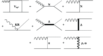
Figure 1: The Born, vector-meson, and $\Delta$-isobar contributions included in the electroproduction potential.

Our model for the pion production potential (i.e., the driving term $V_{\pi\gamma^{*}}$), is given in VladThesis ; CaiaThesis and includes the following tree-level contributions: $N$ direct and crossed terms, $t$- channel $\pi$, $\omega$ and $\rho$ exchanges, the Kroll-Ruderman (contact) term, and the direct and crossed $\Delta$ terms (see Fig.1). The model for the $\pi N$ driving term (i.e. $V_{\pi\pi}$) has been described in detail in piNscatt ; VladThesis .

The possibility of a large negative mass squared of the virtual photon poses a serious problem in the case when one calculates the off-shell elements of the matrix $V_{\pi\gamma^{*}}$ (i.e. $Q^{2}\neq 0$). Namely, singularities are encountered in the integration path when the one-loop integration is performed. In the following we will show how this happens, and give a prescription for avoiding this problem. The singularities only arise in the $t$- and $u$-channel exchange terms.

Consider for instance the denominator of the nucleon propagator in the case of the $u-$channel exchange:

$$S_{N}(p-k)=\frac{p/-k/+m_{N}}{u(Q^{2},W,|\vec{q}\hskip 2.84526pt^{\prime\prime}|,\cos(\theta))-m_{N}^{2}}$$ (1)

where

$$u(Q^{2},W,\vec{q}\hskip 2.84526pt^{\prime\prime},\cos\theta))-m_{N}^{2}$$

$$=\left(E_{N}-k_{0}\right)^{2}-\left(\vec{p}-\vec{k}\right)^{2}-m_{N}^{2}$$

$$=\left(E_{N}-\beta\sqrt{s}+q^{\prime\prime}_{0}\right)^{2}$$

$$-\left(\sqrt{(\vec{p}+\beta\vec{P}-\vec{q}\hskip 2.84526pt^{\prime\prime})^{2}+m_{N}^{2}}\right)^{2},$$ (2)

where $m_{N}$, $m_{\pi}$ are the masses of the nucleon and pion, respectively, $W=\sqrt{s}=P_{\mu}\cdot P^{\mu}$ is the total CM energy of the system, and the relative intermediate energy and momentum are designated by $q^{\prime\prime}_{o}$ and $\vec{q^{\prime\prime}}$ respectively. In Eq. (II) we have made use of the fact that the incoming nucleon has 4-momentum defined by $p^{\mu}=(E_{N},\vec{p})$ (it is fully on-shell), and the outgoing $\pi$ has 4-momentum $k^{\mu}=(k_{0},\vec{k})$, which written in terms of the relative 4-momentum of the outgoing channel has the energy $k_{0}=\beta\sqrt{s}-q^{\prime\prime}_{0}$ and the 3-momentum $\vec{k}=\beta\vec{P}-\vec{q}\hskip 2.84526pt^{\prime\prime}$, where the Lorentz scalars $\alpha$ and $\beta$ are: $\alpha=p\cdot P/s=(s+m_{N}^{2}-m_{\pi}^{2})/2s$ and $\beta=k\cdot P/s=(s-m_{N}^{2}+m_{\pi}^{2})/2s$. We have also assumed that all the kinematics are in the CM frame (i.e., $P^{\mu}=(P^{0},0)=(\sqrt{s},0)$). In this frame, and from kinematics considerations the asymptotic energies of the incoming nucleon and outgoing pion are: $\omega_{\pi}=\left(W^{2}-m_{N}^{2}+m_{\pi}^{2}\right)/2W,$ and $E_{N}=\left(W^{2}+m_{N}^{2}+Q^{2}\right)/2W,$ respectively. The on-shell 3-momentum of the incoming nucleon is $|\vec{p}|=\sqrt{E_{N}^{2}-m_{N}^{2}}$.

The problem of singularities arises when the denominator of the propagator described by the function

$$f = \left[E_{N}-\omega_{\pi}+q^{\prime\prime}_{0}-\sqrt{\left(\vec{p}+\vec{q}\hskip 2.84526pt^{\prime\prime}\right)^{2}+m_{N}^{2}}\right]$$

$$\times \left[E_{N}-\omega_{\pi}+q^{\prime\prime}_{0}+\sqrt{\left(\vec{p}+\vec{q}\hskip 2.84526pt^{\prime\prime}\right)^{2}+m_{N}^{2}}\right],$$

vanishes. Note that in the equal time approximation which we use for the real photon case, $q_{0}^{\prime\prime}=0$. The relative asymptotic energy of the nucleon-pion system is given by:

$$E_{N}-\omega_{\pi}=\frac{2m_{N}^{2}-m_{\pi}^{2}+Q^{2}}{2W},$$ (4)

while the square root term ranges from $m_{N}$ to $\infty$ as the integration variable $|\vec{q}\hskip 2.84526pt^{\prime\prime}|$ ranges over all possible values. Since the minimum value of $W$ is $m_{N}+m_{\pi}$, the function $f$ cannot vanish for $Q^{2}=0$. (Note that it is the first term in $f$ which could possibly have a zero, but for $Q^{2}=0$ this term is always negative.) However, as $Q^{2}$ increases and $E_{N}-\omega_{\pi}$ becomes larger (by the addition of $Q^{2}/2W$ as compared to the $Q^{2}=0$ case), the first term in $f$ can vanish. It vanishes at the smallest value of $Q^{2}/2W$ when $\vec{p}$ and $\vec{q}\hskip 2.84526pt^{\prime\prime}$ are antiparallel and equal in magnitude.

II.1 $Q^{2}/2W$ choice

The singularity in the $u$-channel nucleon exchange can be evaded by fixing the relative energy $q_{0}^{\prime\prime}=-Q^{2}/2W$, instead of to zero as in the equal-time reduction. This choice has the advantage that the propagators in the $u$-channel exchanges are not modified at the photon point. Similar considerations also apply for the case of the $u-$channel $\Delta$ exchange, $t-$channel $\pi$, $\rho$, $\omega$ exchanges, as well as for the case of the hadronic form factors, such as the pion (monopole), and the rho and omega (one boson) form factors. The same choice for $q_{0}^{\prime\prime}$ works for the u-channel $\Delta$ exchange while for the $t$-channel terms and hadronic form factors, one must choose $q_{0}^{\prime\prime}=+Q^{2}/2W$. We shall refer to these modifications of the propagators and form factors as the $Q^{2}/2W$ approximation.

The main objection to this choice would be that it violates current conservation even at the on-shell values of the potential matrix ($V_{\pi\gamma^{*}}$). This problem could be fixed by a global restoration of the current such as:

$$J^{\mu}\rightarrow{J^{\prime}}^{\mu}(Q^{2})=J^{\mu}-n^{\mu}\frac{q\cdot J}{q\cdot n},$$ (5)

where $J^{\mu}$ is the $4-$component electromagnetic current and $n^{\mu}$ is an arbitrary $4-$vector. However, since one of the main goals of our work was to construct a gauge invariant current, at least for the on-shell tree level, such a restoration of current conservation is unsatisfactory.

Instead, we choose to restore the electromagnetic gauge-invariance in the following way. The isospin decomposition of the pion electroproduction amplitude is done as follows:

$$m^{\mu}_{(T)} = \frac{1}{3}\tau_{a}\tau_{3}m^{\mu}_{(1/2)}+\tau_{a}m^{\mu}_{(0)}$$ (6)

$$+ \left(\delta_{a3}-\frac{1}{3}\tau_{a}\tau_{3}\right)m^{\mu}_{(3/2)}$$

where $\tau$ are the usual Pauli matrices, index a stands for the pion isospin states ($\pi^{\pm}$, $\pi^{0}$) and the lower index, in brackets, refers to the total isospin. Using Eq. (6) one can determine the contribution of each exchange to the isospin decomposed amplitudes.

$$m^{\mu}_{(T=\frac{1}{2})} = 3m_{(s,N)}^{\mu}-m_{(u,N)}^{\mu}+4m_{(t,\pi)}^{\mu}$$ (7a)

$$+ 4m_{(KR)}^{\mu}+m_{(t,\omega)}^{\mu}+2m_{(u,\Delta)}^{\mu}$$

$$m^{\mu}_{(T=\frac{3}{2})} = 2m_{(u,N)}^{\mu}-2m_{(t,\pi)}^{\mu}-2m_{(KR)}^{\mu}$$ (7b)

$$+ m_{(t,\omega)}^{\mu}+\frac{3}{2}m_{(s,\Delta)}^{\mu}+\frac{1}{2}m_{(s,\Delta)}^{\mu}$$

$$m^{\mu}_{(T=0)} = m_{(s,N)}^{\mu}+m_{(u,N)}^{\mu}+m_{(t,\rho)}^{\mu}.$$ (7c)

The gauge invariance of the electromagnetic interactions can be imposed by the current conservation condition, $q_{\mu}\cdot m^{\mu}_{T}=0$, for all values of the isospin: $T=0,$ $\frac{1}{2}$, $\frac{3}{2}$. Due to the violation of current conservation introduced by our approximation in the denominators of the on shell potential matrix $m^{\mu}_{T}$, Eqs. (7) have to be modified accordingly. In the following we introduce the correction terms necessary for each isospin channel at tree level. The following notation will be used for this derivation: the unmodified denominators are denoted by a unprimed symbol, while the modified denominators, which include the ${}^{\prime\prime}x^{\mu}=(Q^{2}/2W,\vec{0})^{\prime\prime}$ approximation, are denoted by a primed symbol. The $u-$ and $t-$channel denominators and the hadronic form factor of the exchanged pion can be written:

$$d_{u} = p_{u}\cdot p_{u}-m_{N}^{2}$$

$$d_{u^{\prime}} = (p_{u}-x)\cdot(p_{u}-x)-m_{N}^{2},$$ (8a)

$$d_{t} = p_{t}\cdot p_{t}-m_{\pi}^{2}$$

$$d_{t^{\prime}} = (p_{t}+x)\cdot(p_{t}+x)-m_{\pi}^{2},$$ (8b)

$$d_{f_{\pi}} = p_{t}\cdot p_{t}-\Lambda_{\pi}^{2}$$

$$d_{f_{\pi}^{\prime}} = (p_{t}+x)\cdot(p_{t}+x)-\Lambda_{\pi}^{2},$$ (8c)

where $p_{u}=(p-k)^{\mu}$ and $p_{t}=(q-k)^{\mu}$. From Eqs. (8) the following relationships between denominators result:

$$d_{u^{\prime}}-d_{u} = q_{\mu}\cdot q^{\mu}\Phi$$ (9a)

$$d_{t^{\prime}}-d_{t} = q_{\mu}\cdot q^{\mu}\Psi$$ (9b)

$$d_{f_{\pi}^{\prime}}-d_{f_{\pi}} = q_{\mu}\cdot q^{\mu}\Psi$$ (9c)

where

$$\Phi = \left(Q^{2}+4m_{N}^{2}-2m_{\pi}^{2}\right)/\left(4W^{2}\right),$$ (10)

$$\Psi = \left(Q^{2}+2m_{\pi}^{2}\right)/\left(4W^{2}\right).$$ (11)

Using Eq. (9) the u and t-channels propagators, and the pion form factor in our approximation write:

$$S_{N}^{\prime}(p_{u}) = S_{N}(p_{u})\left(d_{u}/d_{u^{\prime}}\right)$$ (12a)

$$S_{\pi}^{\prime}(p_{t}) = S_{\pi}(p_{t})\left(d_{t}/d_{t^{\prime}}\right)$$ (12b)

$$f_{\pi}^{\prime}(p_{t}) = f_{\pi}(p_{t})\left(d_{f_{\pi}}/d_{f_{\pi}^{\prime}}\right)^{2}.$$ (12c)

Current conservation has to be satisfied by the isospin projected on shell amplitudes (Eqs. (7)) separately. Since the resonant contributions as well as rho and omega exchanges satisfy the condition by their Lorentz structure, then the problem reduces just to the Born terms (i.e. nucleon direct and crossed terms, pion and Kroll-Rudermann terms). Using the modifications introduced in Eqs. (7) and Eqs. (9), and constructing the invariant $q_{\mu}\cdot m^{\mu}_{T}$ for each isospin separately the following violating terms result:

$$q_{\mu}\cdot\Delta m^{\mu}_{\frac{1}{2}} = \left[3+\frac{d_{u}}{d_{u^{\prime}}}-4\frac{d_{t}}{d_{t^{\prime}}}\left(\frac{d_{f_{\pi}}}{d_{f_{\pi}^{\prime}}}\right)^{2}\ \right]\gamma_{5}k/$$ (13a)

$$+ 4\left[\frac{d_{t}}{d_{t^{\prime}}}\left(\frac{d_{f_{\pi}}}{d_{f_{\pi}^{\prime}}}\right)^{2}-1\right]\gamma_{5}q/$$

$$q_{\mu}\cdot\Delta m^{\mu}_{\frac{3}{2}} = -2\left[\frac{d_{u}}{d_{u^{\prime}}}-\frac{d_{t}}{d_{t^{\prime}}}\left(\frac{d_{f_{\pi}}}{d_{f_{\pi}^{\prime}}}\right)^{2}\right]\gamma_{5}k/$$ (13b)

$$- 2\left[\frac{d_{t}}{d_{t^{\prime}}}\left(\frac{d_{f_{\pi}}}{d_{f_{\pi}^{\prime}}}\right)^{2}-1\right]\gamma_{5}q/$$

$$q_{\mu}\cdot\Delta m^{\mu}_{0} = \left(1-\frac{d_{u}}{d_{u^{\prime}}}\right)\gamma_{5}k/$$ (13c)

After some straightforward algebra in Eqs. (13) the analytical terms necessary for correcting the violation of the current conservation, introduced by our approximation, for the on-shell amplitude are:

$$\Delta m^{\mu}_{\frac{1}{2}} = \frac{\gamma_{5}k/\Phi q^{\mu}}{d_{u^{\prime}}}+\frac{-4\Psi q^{\mu}\gamma_{5}(k/-q/)}{d_{t^{\prime}}}\Omega$$ (14a)

$$\Delta m^{\mu}_{\frac{3}{2}} = \frac{-2\gamma_{5}k/\Phi q^{\mu}}{d_{u^{\prime}}}+\frac{2\Psi q^{\mu}\gamma_{5}(k/-q/)}{d_{t^{\prime}}}\Omega$$ (14b)

$$\Delta m^{\mu}_{0} = \frac{-\gamma_{5}k/\Phi q^{\mu}}{d_{u^{\prime}}}$$ (14c)

where

$$\Omega=1-\frac{(d_{t^{\prime}}-Q^{2}\Psi)(2d_{f_{\pi}^{\prime}}+Q^{2}\Psi)}{d_{f_{\pi}^{\prime}}^{2}}$$ (15)

Comparing the isospin factors from Eqs. (14) with those from Eqs. (7) one can exactly identify where each of the contributions from Eqs. (14) has to be incorporated into the calculations. Notice that, as expected, they do not have an effect on the transverse components of the current, hence only the longitude multipoles would be affected by this correction.

While these additional terms clearly restore current conservation at tree level, when we carry out the full dynamical calculation using this procedure or the spectator approximation, we also impose current conservation numerically in the off-shell contributions. We confirmed that the use of a numerical restoration of current conservation at the tree level reproduced the same results as given by the analytical results given above.

II.2 Spectator choice

Previously electroCaia ; CaiaThesis we have used a different method of avoiding the particle-exchange singularities namely the spectator approximation Gross made in the electroproduction potential. As pointed out in Refs. GrS93 ; PaT99 the choice of the spectator particle depends on whether the potential is of the $t$-channel or $u$-channel exchange. For the $u-$channel exchange the outgoing pion is the spectator and therefore should be placed on the mass shell. Then the outgoing nucleon has the energy:

$$E_{N^{\prime}}=W-\sqrt{\vec{q}\hskip 2.84526pt^{\prime\prime 2}+m_{\pi}^{2}}.$$ (16)

Under the spectator approximation the first term in Eq. (II) becomes equal to $W-2\sqrt{\vec{q}\hskip 2.84526pt^{\prime\prime 2}+m_{\pi}^{2}}-\sqrt{(\vec{p}+\vec{q}\hskip 2.84526pt^{\prime\prime})^{2}+m_{N}^{2}}$, which remains negative for all values of $|\vec{q}\hskip 2.84526pt^{\prime\prime}|$.

If the potential is of the form of $t-$channel exchange the outgoing nucleon is set on its mass shell. Thus the outgoing pion energy is:

$$\omega_{\pi}=W-\sqrt{\vec{q}\hskip 2.84526pt^{\prime\prime 2}+m_{N}^{2}},$$ (17)

which also avoids the singularities in the $t$-channel terms. An advantage of the spectator approximation is that the on-shell potential matrix ($V_{\pi\gamma^{*}}$) does not violate current conservation, since this approximation, at the tree level, corresponds to the asymptotic kinematics.

The main disadvantage of the spectator approximation is that it modifies the ${\it on-shell}$ behavior even at the photon point, where no anomalous singularities arise in the u-channel and t-channel terms. In order to describe the $Q^{2}=0$ data in the spectator approximation, it is necessary to refit some of the electromagnetic couplings (the most dramatic change arose in the magnetic coupling of $\Delta$, $G_{M}$). We have done this refitting and all the results presented in electroCaia ; CaiaThesis were calculated using this approximation.

III Results and Discussion

Using the $Q^{2}/2W$ approximation with the restoration of current conservation as described above, we have fitted the major electroproduction multipoles that have been extracted from experiment using the coupling constants determined by pion photoproduction.

The parametrization of the $\gamma N\Delta$ form factors we universally use the form as in electroCaia :

$$G_{I}(Q^{2})=g_{I}\,\frac{1+(Q^{2}/A_{I})\,e^{-Q^{2}/B_{I}}}{(1+Q^{2}/\Lambda_{I})^{2}}\,,I=M,\,E,\,C.$$ (18)

Here we have built in a constraint from perturbative QCD (pQCD) such that these form factors fall as $Q^{-4}$ (modulo logs) for asymptotically large $Q$, see e.g. Carlson98 . In Table 1 are shown the parameters we used in the $N\leftrightarrow\Delta$ form factors using the spectator approximation ($II$), while ($I$) denotes the same parameters using our $Q^{2}/2W-$modification.

	$g_{I(II)}$	$\Lambda_{I(II)}$	$A_{I(II)}$	$B_{I(II)}$
$G_{M}$	2.67(3.10)	0.71(0.60)	1.21(1.02)	1.40(1.20)
$G_{E}$	0.11(0.05)	0.50(0.50)	$-1.10(-1.10)$	$2.00(2.00)$
$G_{C}$	-0.38(-0.18)	0.82(0.78)	$-0.90(-0.90)$	1.00(1.00)

Table 1: Parameters used in the $N\leftrightarrow\Delta$ transition form factors to fit $M_{1+}^{(3/2)}$, $R_{EM}$ and $R_{SM}$. ($I$) $\pm Q^{2}/2W$ modification in the u- and t-channel terms and ($II$) spectator approximation.

In Fig. 2 we plot the $Q^{2}$ dependence of the determined electromagnetic form factors in comparison with the standard dipole form factor $F_{D}(Q^{2})$ using $\Lambda$=$0.71$ $GeV^{2}$. The solid lines are the form factors determined in the $Q^{2}/2W-$approximation, while the dashed lines are the same form factors determined using the spectator approximation. Note that all the form factors are normalized to $1$ at the photon point and that the coupling constants for the two fits are different as given in Table I. One sees that the magnetic form factor $G_{M}(Q^{2})$, in both parameterizations, is overall harder than the dipole at low $Q^{2}$, but it tends toward the dipole values at higher $Q^{2}$, and the two different methods of regularizing the scattering equation lead to moderate effects in the $Q^{2}$ dependence of the form factor. The electric and Coulomb form factors $G_{E}(Q^{2})$ and $G_{C}(Q^{2})$ start much softer than the dipole; but $G_{E}$ at higher $Q^{2}$ tends to return to $F_{D}$, while $G_{C}(Q^{2})$ remains a fraction of $F_{D}$ at high $Q^{2}$. Unlike the magnetic case, both the electric and Coulomb form factors $G_{E}$ and $G_{C}$ have almost the same $Q^{2}$ dependence in both fits. Note that in all cases the overall trend of the $N\leftrightarrow\Delta$ transition form factors as a function of $Q^{2}$ is similar. We can consider the differences as a measure of the uncertainty of our model.

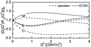
Figure 2: The $Q^{2}$ dependence of the determined $N\rightarrow\Delta$ electromagnetic form factors divided by the dipole form factor, at $W=1.232$ $GeV$.

We have been trying to determine quantitatively the effect of the two approaches used in avoiding the singularities in the u- and t-channel terms. Why do the coupling constants have to be modified from one approach to the other? The method of avoiding the singularities affects only the u- and t-channel contributions. Hence, in Fig. 3 we plot our calculations of the resonant multipoles with the full rescattering model, but in the driving term $V_{\pi\gamma^{*}}$ we include just the pion pole (right panel) contribution (t-channel pion exchange) or just the nucleon u-channel exchange (left panel). The t-channel contribution to the $M_{1+}$ multipole is weakly affected by this modification, while the u-channel changes significantly. This shift results in $g_{M}$ changing from 2.67 to 3.10. The contribution to the $E_{1+}$ multipole at low $Q^{2}$ between model ($I$) and model ($II$) is quite large, resulting in $g_{E}$ changing from 0.112 to 0.048. The differences in the two models at higher $Q^{2}$ are not so large since the effects in the t- and u-channel terms partially cancel. The largest effect is in the $S_{1+}$ multipole. The u-channel contribution varies significantly at low $Q^{2}$ between models ($I$) and ($II$), while at larger $Q^{2}$ it is the t-channel contribution which varies. Using the $Q^{2}=0$ results we had to change $g_{C}$ from -0.38 to -0.18.

Figure 3: Nucleon u-channel (left) and pion t-channel (right) contributions at $W=1.232$ $GeV$ for the resonant multipoles. Solid lines are the multipoles determined using $Q^{2}/2W$ approximations while dashed lines represent the same calculation using spectator approximation. See text for explanations.

Depending on the size of the u- and t-channel contributions to the various multipoles, the values at $Q^{2}=0$ can change significantly and the extracted $Q^{2}$ dependence for $G_{M}$, $G_{E}$ and $G_{C}$ may change from model ($I$) to model ($II$). Fortunately, the overall $Q^{2}$ dependence as shown in Fig. 2 is not changed very much. The nucleon exchange term has a larger effect in the $M_{1+}$ than the pion pole, in fact, the u-channel change leads to a modification of the shape of the fitted $G_{M}(Q^{2})$. In the case of the $E_{1+}$ quadrupole, the $Q^{2}$ dependence is not affected in any of the instances, hence we did not have to refit the $Q^{2}$ dependence of $G_{E}(Q^{2})$. The $Q^{2}$ dependence of $G_{C}(Q^{2})$ had to be slightly modified since we see an overall strengthening of both the pion pole and nucleon crossed terms (above $Q^{2}\approx 1$ $(GeV/c)^{2}$) from model ($II$) to model ($I$), hence we had to make $G_{C}(Q^{2})$ slightly harder from model ($II$) to model ($I$). We did not plot the effects of these two models in the $\Delta$ crossed term but we analyzed them, and as expected, they did not play an important role in the resonant multipoles (most of the $\Delta$ contribution to the resonant multipoles comes from the direct and the Born terms).

In Fig. 4 and Fig.5 we compare our calculations with some recent results from CLAS alt ; siglt . This asymmetry measurement is important in determining the $t-$channel pion pole and contact Born terms contributions in $\pi^{+}n$, which otherwise are weak in the $\pi^{0}p$ channel. Measurements of beam asymmetry $A_{LT^{\prime}}$ where made only for the neutral channel, but since in this reaction the non-resonant amplitude strongly interferes with the imaginary part of the dominant $\Delta(1232)$ $M_{1+}^{(3/2)}$ it is difficult to extract the information about the non-resonant contribution to the observables. The resulting amplitude for $\pi^{0}p$ is strongly dependent on the rescattering correction and largely dependent on the way the model generates the width of the resonance.

The calculated angular distribution of $\sigma_{LT^{\prime}}$ for the $\pi^{+}n$ channel show a strong forward peaking for energies around the $\Delta$, in contrast to $\pi^{0}p$ channel which shows backward peaking. In Fig. 4 and Fig. 5 we plot the asymmetry $A_{LT^{\prime}}$ and the longitudinal-transverse polarized structure function $\sigma_{LT^{\prime}}$, respectively. The relationship between these two quantities, following the reference MAID_polarization conventions, is as follows:

$$A_{LT^{\prime}}=\sqrt{2\epsilon_{L}(1-\epsilon)}R_{LT^{\prime}}\sin\phi_{\pi}/\sigma_{0},$$ (19)

where

$$\sigma_{0} = R_{T}+\epsilon_{L}R_{L}+\sqrt{2\epsilon_{L}(1+\epsilon)}R_{TL}\cos\phi_{\pi}$$ (20)

$$+ \epsilon R_{TT}\cos 2\phi_{\pi},$$

where $R_{i}$ ($i=T,L,LT,TT$) are the response functions, $\epsilon=\left(1+2|{\bf q}|^{2}/Q^{2}\tan^{2}\left(\theta_{e}/2\right)\right)^{-1}$ is the degree of transverse polarization and $\epsilon_{L}=\left(Q^{2}/\omega^{2}\right)\epsilon$ is the degree of longitudinal polarization of the virtual photon. Therefore the longitudinal-transverse polarized structure function shown in Fig. 4 is: $\sigma_{LT^{\prime}}=R_{LT^{\prime}}/\sin\theta_{\pi}$, which is written in terms of the electromagnetic multipoles,

$$R_{LT^{\prime}}= - \sin\theta_{\pi}Im\{(F_{2}^{*}+F_{3}^{*}+\cos\theta_{\pi}F_{4}^{*})F_{5}$$ (21)

$$+ (F_{1}^{*}+F_{4}^{*}+\cos\theta_{\pi}F_{3}^{*})F_{6}\},$$

where $F_{i}$ with $i=1,\ldots,6$, are the CGLN amplitudes CGLN which are defined in the appendix of MAID_polarization .

Figure 4: $\sigma_{LT^{\prime}}$ versus $\cos\theta_{\pi}$ for $p(e,e^{\prime}n)\pi^{+}$ and $p(e,e^{\prime}p)\pi^{0}$ at $Q^{2}=0.4(GeV/c)^{2}$. The data points are from siglt ; alt . The lines are the same as in Fig.3

Figure 5: Beam asymmetry versus $\phi_{\pi}$ for $p(e,e^{\prime}n)\pi^{+}$ at $Q^{2}=0.4(GeV/c)^{2}$, $W=1.22$ $GeV$ and for fixed $\theta$. The data points are from alt and the lines are the same as in Fig.3

The two approximations (solid lines is the $Q^{2}/2W$-approximation and dashed line is the spectator approximation) are used in our calculations and a fairly good agreement is obtained in both cases. The largest difference can be noticed in the case of the asymmetry $A_{LT^{\prime}}$ for the neutral channel for c.m. total energy equal to the $\Delta$ mass, while for the other kinematics there is no practical difference. Since these observables are directly proportional to the longitudinal component of the electromagnetic current, then the overall difference can be a direct measure of the uncertainty of our model related to the theoretical error introduced by either of the approximations.

In view of the upcoming data from JLab for higher values of the $Q^{2}$, in Figs. 6 and 7 we show the prediction of our model for differential cross sections although we only fit our $\Delta$ electromagnetic form-factors up to $Q^{2}=4(GeV/c)^{2}$ (see electroCaia ). For the differential cross section both approximations give very similar results, proving once again that the cross section is not sensitive enough to possible theoretical errors in the model.

Figure 6: Differential cross section versus $\phi_{\pi}$ for $p(e,e^{\prime}p)\pi^{0}$ at $Q^{2}=5(GeV/c)^{2}$, $W=1.23$ $GeV$ and for fixed $\theta$. The lines are the same as in Fig.3

Figure 7: Differential cross section versus $\phi_{\pi}$ for $p(e,e^{\prime}p)\pi^{0}$ at $Q^{2}=6(GeV/c)^{2}$, $W=1.23$ $GeV$ and for fixed $\theta$. Only the $Q^{2}/2W$ approximation is shown, since the spectator gives almost identical predictions.

IV Conclusions

A dynamical model for pion electro-production was first introduced in electroCaia where it was used for determining the $\Delta$ electromagnetic form-factors. The major theoretical uncertainty in our model is the treatment of the u- and t-channel terms in the potential $V_{\pi\gamma^{*}}$. For large $Q^{2}$ (i.e., large negative mass squared of the virtual photon), non-physical singularities occur in these terms when they go off shell in solving the scattering integral equation. We have investigated two approximate ways of solving this problem. The first was the spectator approximation for these diagrams and the second was to modify the relative energy in these diagrams by $\pm Q^{2}/2W$. We have shown that the singularity problem can be partially solved without affecting the $Q^{2}=0$ results by proposing an ad-hoc solution which avoids these poles. Within the theoretical uncertainty of how to regularize the u- and t-channel terms for pion electro-production, this model provides an overall good prediction of the available data up through the first resonance region. Comparison with recent single polarization data also shows fairly good agreement. Furthermore, we predict cross sections at higher $Q^{2}$ that are being analyzed at Jlab. In our view, the $\pm Q^{2}/2W$ approximation with restoration of current conservation provides a good dynamic model for investigating pion electroproduction at large $Q^{2}$. The parameters needed also describe pion photoproduction quite well and allows the two processes to be studied in the same model.

References

- (1) V. V. Frolov et al., Phys. Rev. Lett. 82, 45 (1999).
- (2) K. Joo et al., Phys. Rev. Lett. 88, 12201 (2002).
- (3) G. Blanpied et al. Phys. Rev. Lett. 79, 4337 (1997).
- (4) R. Beck et al., Phys. Rev. C 61, 035204 (2000).
- (5) C. Mertz et al., Phys. Rev. Lett. 86, 2963 (2001).
- (6) R. Arndt, W. Briscoe, I. Strakovsky and R. Workman, arXiv:nucl-th/0301068 [http://gwdac.phys.gwu.edu].
- (7) D. Drechsel, O. Hanstein, S. S. Kamalov and L. Tiator, Nucl. Phys. A 645 (1999) 145 [http://www.kph.uni-mainz.de/MAID].
- (8) T. Sato and T. -S. H. Lee, Phys. Rev. C 54, 2660 (1996); ibid. 63, 055201 (2001).
- (9) S. S. Kamalov and S. N. Yang, Phys. Rev. Lett. 83, 4494 (1999); L. Tiator, D. Drechsel, S. S. Kamalov and S. N. Yang, Eur. Phys. J. A 17, 357 (2003).
- (10) I. G. Aznauryan, Phys. Rev. C 67, 015209 (2003); I. G. Aznauryan et al., Phys. Rev. C 71, 015201 (2005).
- (11) G. L. Caia, V. Pascalutsa, J. A. Tjon and L. E. Wright, Phys. Rev. C69, 035205 (2004).
- (12) V. Pascalutsa and J. A. Tjon, Phys. Rev. C61, 054003 (2000).
- (13) V. Pascalutsa and J. A. Tjon, Phys. Rev. C70, 035209 (2004).
- (14) V. Pascalutsa, PhD Thesis (University of Utrecht, 1998) [Published in: Hadronic J. Suppl. 16, 1 (2001)].
- (15) F. Gross, Phys. Rev. 186, 1448 (1969); Phys. Rev. C 26, 2203 (1982).
- (16) F. Gross and Y. Surya, Phys. Rev. C 47, 703 (1993).
- (17) V. Pascalutsa and J. A. Tjon, Phys. Rev. C 60, 034005 (1999) [arXiv:nucl-th/9907053].
- (18) G. L. Caia, PhD Thesis (Ohio University, 2004) [http://www.ohiolink.edu/etd].
- (19) C. E. Carlson and N. C. Mukhopadhyay, Phys. Rev. Lett. 81, 2646 (1998).
- (20) Dieter Drechsel and Lothar Tiator, J. Phys. G: Nucl. Part. Phys. 18, 449-497 (1992).
- (21) G. F. Chew, M. L. Goldberger, F. E. Low, and Y. Nambu, Phys. Rev. 106, 1345 (1957).
- (22) K. Joo et al., Phys. Rev. C68, 032301(R) (2003).
- (23) K. Joo et al., Phys. Rev. C70, 042201(R) (2004).