Inhomogeneities in the freeze-out of relativistic heavy ion collisions at CERN SPS

Abstract

We study the role of temperature and density inhomogeneities on the freeze-out of relativistic heavy ion collisions at CERN SPS. Especially the impact on the particle abundancies is investigated. The quality of the fits to the measured particle ratios in 158 AGeV Pb+Pb collisions significantly improves as compared to a homogeneous model.

One of the key motivations for the heavy ion programs at GSI, CERN and BNL is to shed light on the QCD phase diagram. More specifically, the aim is to gain a deeper understanding of the physics of the different phases of QCD matter and of the characteristics of the deconfinement and chiral phase transition (cf. Fig. 1).

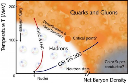
Figure 1: Different phases of strongly interacting matter in the T-$\rho$ plane. Relativistic heavy ion experiments heat and compress ordinary nuclei to high temperatures and densities. Depending on the bombarding energy, the transition to chirally restored quark- and gluon matter happens in different temperature and density regions, where the characteristics of the phase transition are expected to be different. Taken from GSI .

The current picture of the QCD phase diagram is as follows: At vanishing chemical potential ($\mu=0$) finite temperature lattice QCD calculations find a rapid but smooth crossover (see e.g. Brown90 ). At large $\mu$ one has to rely on model calculations, since lattice QCD calculations encounter the fermion sign problem. However, several different model calculations (see Stephanov04 for a summary) suggest a first order phase transition. Combining these two results, the line of first order phase transitions originating at the $T=0$ axis cannot end at $\mu=0$ but at some point in the ($T_{c},\mu_{c}$) plane with finite $\mu$. At this endpoint a second order phase transition is expected. For chemical potentials smaller than $\mu_{c}$ a crossover occurs. This picture is also supported by different extrapolations of lattice QCD to finite chemical potential Allton02 ; Fodor:2001pe .

E.g., in Fodor:2001pe it was found that a line of first-order phase transitions in the $(\mu_{B},T)$ plane ends in a critical point at $T\approx 160$ MeV, $\mu_{B}\approx 360$ MeV (cf. Fig. 2).

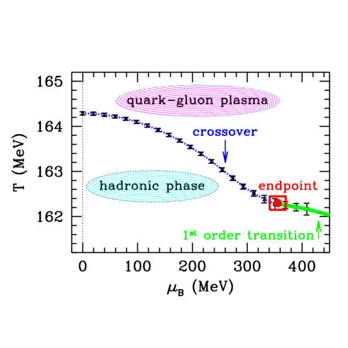
Figure 2: Quark-hadron phase transition as obtained from lattice calculations (at finite chemical potential). Taken from Fodor:2001pe .

Heavy-ion collisions at high energies are hoped to be able to detect that critical point and verify this picture. For high enough energies the phase transition/crossover line should be crossed - the critical energy density is expected to be reached at intermediate SPS energies or the new GSI facility. Since the system takes different paths in the $T-\mu$ or $T-\rho$ plane for different bombarding energies, it is hoped that by varying the beam energy, one can “switch” between the regimes of first-order transition and cross over, respectively (cf. Fig. 1).

But how do we know whether the system passed through a first order phase transition, a crossover, or if no phase change at all occured?

Using a non-equilibrium hydrodynamical simulation it was shown in Paech:2003fe that the expanding fluid develops significant inhomogeneities, if a first order phase transition is crossed. These inhomogeneities should also be present on the decoupling surface of the hadrons.

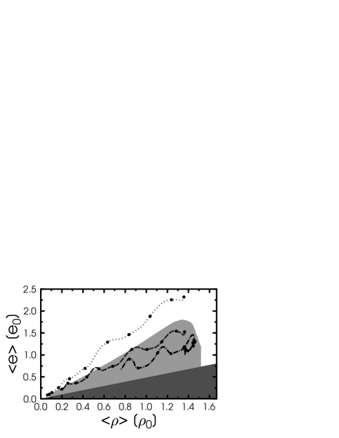
Figure 3: Evolution of the average fluid energy through a crossover (dots), and a weak (dashes) and strong (dash-dots) first order phase transition. The fat dots indicate time intervals of $\approx 1.5$ fm/c. Taken from Paech:2003fe .

Fig. 3 shows the trajectory of the system within the phase diagram for different initial conditions. Depending on these initial conditions, the system either evolves smoothly through a crossover or enters the region corresponding to phase coexistence in the equilibrium phase diagram and thus undergoes a first order phase transition. The resulting RMS fluctuations of the baryon density are shown in figure 4. It can be seen that the amplitude of the density contrast is substantially larger for a strong first order transition (initial energy density $\rm{e}_{\rm{eq}}=1.4e_{0}$) than for a crossover ($\rm{e}_{\rm{eq}}=2.9e_{0}$).

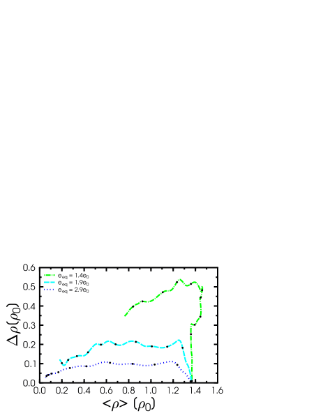
Figure 4: RMS fluctuation of the baryon density with initial conditions chosen such that the system undergoes a crossover (dots), weak (dashes) and strong (dash-dots) first order transition as a function of the average baryon density. The fat dots indicate time intervals of $\approx 1.5$ fm/c. Taken from Paech:2003fe .

That means, that if the particles decouple shortly after the expansion trajectory crosses the line of first order transitions one may expect a rather inhomogeneous (energy-) density distribution on the freeze-out surface (similar, say, to the CMB photon decoupling surface observed by WMAP wmap , see Fig. 5).

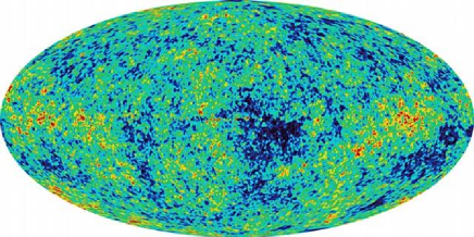
Figure 5: CMB photon decoupling surface observed by WMAP. Dark regions correspond to cooler and brighter regions corrspond to warmer spots. Taken from wmap .

On the other hand, if the system expands through a crossover transition, as expected for collisions at very high energies ($\mu_{B}\simeq 0$, cf. Fig. 1) it may cool smoothly from high to low $T$ and so pressure gradients tend to wash out density inhomogeneities. Similarly, in the absence of phase-transition induced non-equilibrium effects, the predicted initial-state density inhomogeneities iniflucs should be strongly damped.

Unfortunately, if the scale of the inhomogeneities is much smaller than the decoupling volume then they can not be resolved individually, nor will they give rise to large event-by-event fluctuations. However, because of the nonlinear dependence of the hadron densities on $T$ and $\mu_{B}$ they should nevertheless reflect in the event-averaged abundances.

Particle production in relativistic heavy ion collisions has been investigated in several works (see for example thermo ) using (homogeneous) thermodynamical equilibrium calculations. In addition, e.g. in thermo_gammas ; Becattini:2003wp extensions accounting for strange- and light quark non-equlibrium were considered and for example in thermo_int the role of in-medium masses was discussed. Here, we attempt to check whether the experimental data show any signs of inhomogeneities on the freeze-out surface. To do this we investigate an inhomogeneous fireball at (chemical) decoupling. Perhaps the simplest possible ansatz is to employ the grand canonical ensemble and - in extension to the homegeneous models - assume that the intensive variables $T$ and $\mu_{B}$ are distributed according to a Gaussian Dumitru05 . This avoids reference to any particular dynamical model for the formation and the distribution of density perturbations on the freeze-out surface. Also, in this simple model we do not need to specify the probability distribution of volumes $V$. Then, the average density of species $i$ is computed as

$$\overline{\rho}_{i}\;(\overline{T},\overline{\mu}_{B},\delta T,\delta\mu_{B})=$$ (1)

$$\int\limits_{0}^{\infty}dT\;P(T;\overline{T},\delta T)\int\limits_{-\infty}^{\infty}d\mu_{B}\;P(\mu_{B};\overline{\mu}_{B},\delta\mu_{B})~{}\rho_{i}(T,\mu_{B})~{},$$

with $\rho_{i}(T,\mu_{B})$ the actual “local” density of species $i$, and with $P(x;\overline{x},\delta x)\sim$ $\exp\left(-\frac{\left(x-\overline{x}\right)^{2}}{2\;\delta x^{2}}\right)$ the distribution of temperatures and chemical potentials on the freeze-out surface. Feeding from (strong or weak) decays is included by replacing $\overline{\rho}_{i}\rightarrow\overline{\rho}_{i}+B_{ij}\;\overline{\rho}_{j}.$ The implicit sum over $j\neq i$ runs over all unstable hadron species, with $B_{ij}$ the branching ratio for the decay $j\to i$. For the present analysis we computed the densities $\rho_{i}(T,\mu_{B})$ in the ideal-gas approximation. The resonances are included up to 1.5 GeV in mass for the mesons and up to 2 GeV for the baryons. The finite widths of the resonances were not taken into account and unknown branching ratios in the particle data book were excluded from the feeding. Furthermore, we use a four-dimensional table with 5 MeV steps in $T$ and $\delta T$ and $10$ MeV steps in $\mu$ and $\delta\mu$. This finite grid-size of course limits our accuracy in determining the best fits. However, our approach should be well suited to investigate the qualitative behavior of the parameters $\delta T$ and $\delta\mu_{B}$ and whether they can significantly improve the agreement with the experimental data.

The data used in our analysis are the particle multiplicities measured by the NA49 collaboration in $\sqrt{s_{NN}}=17.3$ GeV Pb+Pb collisions at CERN SPS. We use midrapidity and $4\pi$ data, both as compiled in Becattini:2003wp .

Using these data, we perform a $\chi^{2}$ fit. I.e., we determine the minimal value of

$$\chi^{2}=\sum_{i}{\left(r_{i}^{exp}-r_{i}^{model}\right)^{2}}/{\sigma_{i}^{2}},$$ (2)

where $r_{i}^{exp}$, $r_{i}^{model}$ denote the experimentally measured and the calculated particle ratios, respectively, and $\sigma_{i}^{2}$ is the experimental error. We compare two cases: On the on hand the homogeneous fit, where the values of $\delta T$ and $\delta\mu$ are set to zero, and on the other hand the inhomogeneous fit, where we allow for finite values of $\delta T$ and $\delta\mu$.

We find that the fits improve (lower $\chi^{2}/\rm{dof}$) substantially if $\delta T$, $\delta\mu_{B}$ are not forced to zero. Table 1 shows the resulting best fits, with and without finite widths of the $T$ and $\mu_{B}$ distributions.

	$\overline{T}$	$\overline{\mu}_{B}$	$\delta T$	$\delta\mu_{B}$	$\chi^{2}/\mbox{dof}$
SPS-158	$155\pm 5$	$200\pm 10$	0	0	40.4/8
(mid)	$105\pm 5$	$230\pm 15$	$35\pm 5$	$80\pm 40$	11.2/6
SPS-158	$145\pm 5$	$210\pm 15$	0	0	40.0/11
($4\pi$)	$100\pm 5$	$260\pm 15$	$30\pm 5$	$190\pm 35$	5.7/9

Table 1: Best fit parameters and $\chi^{2}/dof$ to SPS 158 AGeV midrapidity and $4\pi$ data, measured by the NA49 collaboration. The cases $\delta T=\delta\mu=0$ corresponds to the homogeneous freeze-out model and those with finite values for $\delta T,\delta\mu$ correspond to the inhomogeneous model.

As can be seen, for $4\pi$ data the resulting best fit $\chi^{2}/dof$ values are approximately 3.6 for the homogeneous fit and 0.63 for the inhomogeneous fit. For midrapidity data we obtain $\chi^{2}/dof\approx 5.1$ for the homogeneous and $\chi^{2}/dof\approx 1.9$ for the inhomogeneous case. I.e., for both data sets the $\chi^{2}$ per degree of freedom is considerably reduced by allowing for inhomogeneities or finite widths of the $T$- and $\mu$-distributions, respectively. In other words: for midrapidity as well as for $4\pi$ data $\delta T$ and $\delta\mu$ represent significant paramters. Error estimates for the parameters (confidence intervals) are obtained from the projection of the regions in parameter space defined by $\chi^{2}\leq\chi^{2}_{min}+1$ onto each axis. This corresponds to a confidence level of $68.3\%$ if the errors are normally distributed. As shown in table 1, within this error estimate, the best-fit values for $\delta T$ and $\delta\mu$ are significantly greater than 0.

The resulting particle ratios for the different fits are compared to the experimental $4\pi$ data in figures 6 and 7. As can be seen especially in figure 7, significant improvement compared to the homogeneous freeze-out model is obtained for the Kaons, the mulit-strange baryons, but also for the $\phi$, which couples only to temperature fluctuations.

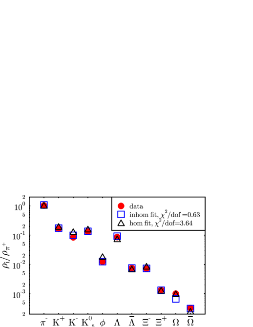
Figure 6: Particle ratios ($4\pi$, compiled in Becattini:2003wp ) as measured by the NA49 collaboration in SPS 158 AGeV Pb+Pb collisions compared to the homogeneous fit ($\delta T=\delta\mu=0$) and the inhomogeneous fit ($\delta T,\delta\mu$ free parameters).

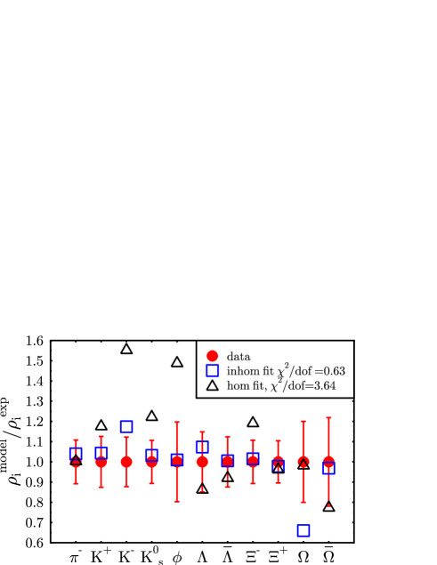
Figure 7: Fitted particle densities divided by the corresponding measured $4\pi$ particle density (NA49 collaboration, Pb+Pb @ SPS 158 AGeV, compiled in Becattini:2003wp ) for the homogeneous ($\delta T=\delta\mu=0$) and the inhomogeneous fit ($\delta T,\delta\mu$ free parameters).

As can be seen from table 1, the inhomogeneous fits return significantly lower mean temperature $\overline{T}$. However, these do not correspond to the “mean” emission temperature of the particles. The actual particle emission distribution is obtained by folding the assumed Gaussian $(T,\mu)$-freeze-out distribution (dashed line in Fig. 8 and 9) with the ideal gas density distribution for a given particle species. The resulting normalized probability distributions read:

$$D_{i}(T,\overline{T},\overline{\mu}_{B},\delta T,\delta\mu_{B})=$$ (3)

$$\frac{P(T;\overline{T},\delta T)\int\limits_{-\infty}^{\infty}d\mu_{B}\;P(\mu_{B};\overline{\mu}_{B},\delta\mu_{B})~{}\rho_{i}(T,\mu_{B})~{}}{\overline{\rho}_{i}\;(\overline{T},\overline{\mu}_{B},\delta T,\delta\mu_{B})}.$$

$$D_{i}(\mu_{B},\overline{T},\overline{\mu}_{B},\delta T,\delta\mu_{B})=$$ (4)

$$\frac{P(\mu_{B};\overline{\mu}_{B},\delta\mu_{B})\int\limits_{-\infty}^{\infty}d\mu_{B}\;P(T;\overline{T},\delta T)~{}\rho_{i}(T,\mu_{B})~{}}{\overline{\rho}_{i}\;(\overline{T},\overline{\mu}_{B},\delta T,\delta\mu_{B})}.$$

They are shown in figure 8 and 9, respectively.

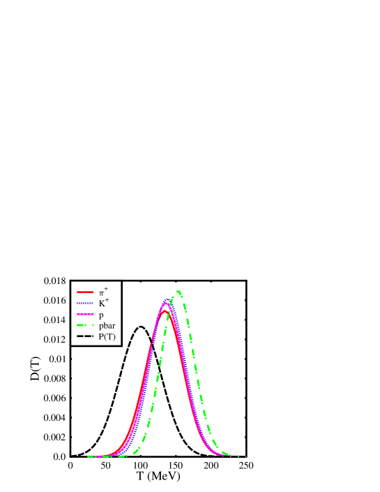
Figure 8: Relative particle density versus temperature for $\pi,K,p$ and $\bar{p}$ which are obtained from folding the underlying Gaussian $(T,\mu)$-freeze-out distribution (dashed line) with the ideal-gas particle density distribution.

As expected from the temperature distribution we observe that the particle emission distributions are shifted towards higher temperatures. How much the distribution is shifted depends on the mass and the chemical potential of the corresponding particle species. The probability distributions of the different particle species versus chemical potential are shifted to larger chemical potentials for the particles and to lower chemical potentials for the antiparticles.

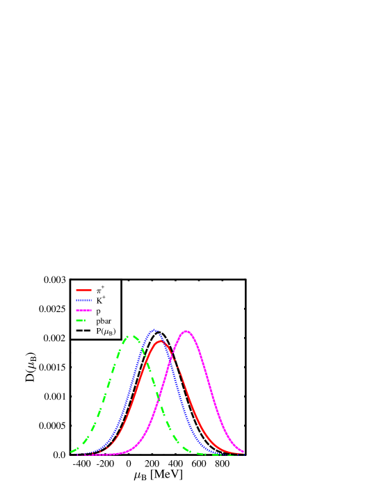
Figure 9: Relative particle density versus chemical potential for $\pi,K,p$ and $\bar{p}$.

Thus, from the finite widths of the Gaussian, different particle emission distributions, with different peaks for different particle species, result. The corresponding means of the distributions can be evaluated as

$$<T>_{i} = \int dT\;T\;D_{i}(T,\overline{T},\overline{\mu}_{B},\delta T,\delta\mu_{B}),$$ (5)

$$<\mu_{B}>_{i} = \int d\mu_{B}\;\mu_{B}\;D_{i}(\mu_{B},\overline{T},\overline{\mu}_{B},\delta T,\delta\mu_{B}).$$ (6)

The resulting means of the distributions for our analysis of the SPS 158 AGeV data are shown in table 2.

SPS 158	$p$	$\bar{p}$	$K^{+}$	$K^{-}$	$\Omega$	$\bar{\Omega}$
$<T>$ [MeV] (mid)	157	170	152	150	164	180
$<\mu_{B}>$ [MeV] (mid)	268	191	237	222	234	225
$<T>$ [MeV] ($4\pi$)	136	153	140	139	151	165
$<\mu_{B}>$ [MeV] ($4\pi$)	487	22	306	213	277	206

Table 2: Mean temperature and chemical potential of various particle species for the inhomogeneous freeze-out.

Again it can be seen that the antiparticles are mainly emitted from regions with small chemical potentials while the particles mainly originate from high chemical potential regions. The mean emission temperatures are in the range of 150-180 MeV for the midrapidity data and of 136-165 for the $4\pi$ data. One sees that the antiparticles emerge in general from hotter regions than the particles.

In conclusion, we find that allowing for inhomogeneities in the freeze-out temperature and chemical potential in an ideal gas description of particle production in heavy ion collisions, significantly improves (lower $\chi^{2}/dof$) the description of experimental data at SPS 158 AGeV. It follows that the bulk of the particles originates from different density and temperature regions than the corresponding anti-particles. Hence, our results suggest that the decoupling surface might not be very well “stirred”. Furthermore, inhomogeneities appear to cure some deficencies of homogeneous freeze-out models and they might represent a potential variable to connect the measured particle abundances to the course of the expansion of the system. The investigation of lower SPS and RHIC energies within our model is under way Dumitru05b . Furthermore, in a future comprehensive analysis, the inhomogeneities should be generated within a dynamical description.

Acknowledgements

It is a pleasure to thank the organizers of the ”XLIII International Winter Meeting On Nuclear Physics” in Bormio for the opportunity to present our results and my collaborators Adrian Dumitru and Licinio Portugal. Furthermore I like to thank Carsten Greiner for very fruitful discussions.

References

-
(1)
http://www.gsi.de
- (2) F. R. Brown et al., Phys. Rev. Lett. 65 (1990) 2491.
- (3) M. A. Stephanov, Prog. Theor. Phys. Suppl. 153 (2004) 139 [arXiv:hep-ph/0402115].
- (4) C. R. Allton et al., Phys. Rev. D 66 (2002) 074507 [arXiv:hep-lat/0204010].
- (5) Z. Fodor and S. D. Katz, JHEP 0404 (2004) 050.
- (6) K. Paech, H. Stöcker and A. Dumitru, Phys. Rev. C 68 (2003) 044907; K. Paech and A. Dumitru, arXiv:nucl-th/0504003. O. Scavenius, A. Dumitru and A. D. Jackson, arXiv:hep-ph/0103219, figs. 5,6.
-
(7)
http://map.gsfc.nasa.gov/m_mm.html
- (8) M. Gyulassy, D. H. Rischke and B. Zhang, Nucl. Phys. A 613, 397 (1997); M. Bleicher et al., Nucl. Phys. A 638 (1998) 391; O. J. Socolowski, F. Grassi, Y. Hama and T. Kodama, Phys. Rev. Lett. 93 (2004) 182301. H. J. Drescher, S. Ostapchenko, T. Pierog and K. Werner, Phys. Rev. C 65 (2002) 054902 [arXiv:hep-ph/0011219].
- (9) E. Fermi, Prog. Theor. Phys. 5 (1950) 570. L. D. Landau, Izv. Akad. Nauk SSSR Ser. Fiz. 17, 51 (1953). D. Hahn and H. Stöcker, Nucl. Phys. A452, 723 (1986). P. Braun-Munzinger, D. Magestro, K. Redlich, and J. Stachel, Phys. Lett. B518, 41 (2001). G. D. Westfall et al., Phys. Rev. Lett. 37, 1202 (1976). L. P. Csernai and J. I. Kapusta, Phys. Rept. 131, 223 (1986). P. Braun-Munzinger, K. Redlich and J. Stachel, arXiv:nucl-th/0304013. W. Florkowski, W. Broniowski and M. Michalec, Acta Phys. Polon. B 33 (2002) 761 [arXiv:nucl-th/0106009].
- (10) J. Rafelski, Phys. Lett. B 262 (1991) 333. J. Rafelski, J. Letessier and A. Tounsi, Acta Phys. Polon. B 27 (1996) 1037 [arXiv:nucl-th/0209080]. F. Becattini, J. Cleymans, A. Keranen, E. Suhonen and K. Redlich, Phys. Rev. C 64 (2001) 024901 [arXiv:hep-ph/0002267]. G. Torrieri, S. Steinke, W. Broniowski, W. Florkowski, J. Letessier and J. Rafelski, arXiv:nucl-th/0404083. J. Rafelski and J. Letessier, Acta Phys. Polon. B 34 (2003) 5791 [arXiv:hep-ph/0309030]. S. Wheaton and J. Cleymans, arXiv:hep-ph/0412031.
- (11) W. Florkowski, W. Broniowski and M. Michalec, Acta Phys. Polon. B 33 (2002) 761 [arXiv:nucl-th/0106009]. D. Zschiesche, S. Schramm, J. Schaffner-Bielich, H. Stocker and W. Greiner, Phys. Lett. B 547 (2002) 7 [arXiv:nucl-th/0209022]. D. Zschiesche, G. Zeeb, K. Paech, H. Stocker and S. Schramm, J. Phys. G 30 (2004) S381.
- (12) A. Dumitru, L. Portugal and D. Zschiesche, arXiv:nucl-th/0502051.
- (13) F. Becattini, M. Gazdzicki, A. Keranen, J. Manninen and R. Stock, Phys. Rev. C 69 (2004) 024905.
- (14) A. Dumitru, L. Portugal and D. Zschiesche, in preparation