A relativistic two-nucleon model for $A(p,K^{+}){{}_{\Lambda}}B$ reaction

Abstract

We investigate the $A(p,K^{+}){{}_{\Lambda}}B$ reaction within a covariant two nucleon model. We focus on amplitudes which are described by creation, propagation and decay into relevant channel of $N^{*}$(1650), $N^{*}$(1710), and $N^{*}$(1720) intermediate baryonic resonance states in the initial collision of the projectile nucleon with one of its target counterparts This collision is modeled by the exchange of $\pi$ as well as $\rho$ and $\omega$ mesons. The bound state nucleon and hyperon wave functions are obtained by solving the Dirac equation with appropriate scalar and vector potentials. Expressions for the reaction amplitudes are derived taking continuum particle wave functions in both distorted wave and plane wave approximations. Detailed numerical results are presented in the plane wave approximation; estimates of the effects of the initial and final state interactions are given in the eikonal approximation. Cross sections of 1 - 2 nb/sr at the peak positions, are obtained for favored transitions in case of heavier targets.
PACS numbers: $25.40.Ve$, $13.75.-n,$, $13.75.Jz$

1 Introduction

$\Lambda$ hypernuclei are the most familiar hypernuclear systems which have been studied extensively by stopped as well as in-flight $(K^{-},\pi^{-})$ reaction [1, 2, 3] and also by $(\pi^{+},K^{+})$ reaction [4, 5]. The kinematical properties of the $(K^{-},\pi^{-})$ reaction allow only a small momentum transfer to the nucleus (at forward angles), thus there is a large probability of populating $\Lambda$-substitutional states ($\Lambda$ assume the same orbital angular momentum as that of the neutron being replaced by it). On the other hand, in the $(\pi^{+},K^{+})$ reaction the momentum transfer is larger than the nuclear Fermi momentum. Therefore, this reaction can populate states with the configuration of an outer neutron hole and a $\Lambda$ hyperon in a series of orbits covering all the bound states. During past years data on the hypernuclear spectroscopy have been used extensively to extract information about the hyperon-nucleon interaction (which could be quite different from the nucleon-nucleon interaction) within a variety of theoretical approaches (see, e.g., [6, 7]).

Alternatively, $\Lambda$-hypernuclei can also be produced with high intensity proton beams via $p+A(N,Z)\rightarrow{{}_{\Lambda}}B(N-1,Z)+n+K^{+}$, $p+A(N,Z)\rightarrow{{}_{\Lambda}}B(N,Z-1)+p^{\prime}+K^{+}$, and $p+A(N,Z)\rightarrow{{}_{\Lambda}}B(N,Z)+K^{+}$ reactions where $N$ and $Z$ are the neutron and proton numbers, respectively, in the target nucleus. In this paper we study the last reaction [to be referred to as $A(p,K^{+}){{}_{\Lambda}}B$] where the hypernucleus ${{}_{\Lambda}}B$ has the same neutron and proton numbers as the target nucleus $A$, with one hyperon added. This reaction is exclusive in the sense that the final channel is a two body system. First set of very preliminary data have already been reported for this reaction on deuterium and helium targets [8]. More measurements for this reaction involving also the heavier targets are expected to be performed at the COSY facility of the Forschungszentrum Jülich [see, e.g., Ref. [9]]. This reaction involves much larger momentum transfer to the nucleus as compared to the $(\pi^{+},K^{+})$ reaction [more than 1.0 GeV/c (see Fig. 1) as compared to only 0.33 GeV/c at the outgoing $K^{+}$ angle of 0^∘]. Therefore, it samples bound state wave functions in a region where they are very small and are unlikely to be reached in other reactions. From the spectroscopic point of view, the states of the hypernucleus ${}_{\Lambda}B$ excited in the $(p,K^{+})$ reaction may have a different type of configuration as compared to those reached in the $(\pi^{+},K^{+})$ reaction. Thus a comparison of informations extracted from the study of two reactions is likely to provide a better understanding of the hypernuclear structure.

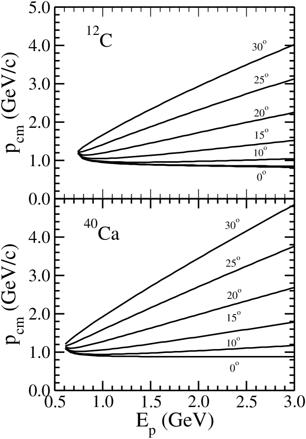
Figure 1: Center-of-mass momentum transfer available to the ($p,K^{+}$) reaction as a function of the laboratory bombarding energy ($E_{p}$) for ¹²C and ⁴⁰Ca targets. For a fixed energy the allowed kinematic region extends from 0^∘ to 180^∘. We have shown here only a few angles.

Theoretical studies of the $A(p,K^{+}){{}_{\Lambda}}B$ reaction are rather sparse and preliminary in nature [10, 11, 12, 13]. They are based on two main approaches; the one-nucleon model (ONM) [Fig. 2(a)] and the two-nucleon model (TNM) [Figs. 2(b) and 2(c)]. In the ONM the incident proton first scatters from the target nucleus and emits a (off-shell) kaon and a $\Lambda$ hyperon. Subsequently, the kaon rescatters into its mass shell while the hyperon gets captured into one of the (target) nuclear orbits. Thus there is only a single active nucleon (impulse approximation) which carries the entire momentum transfer to the target nucleus. This makes this model extremely sensitive to details of the bound state wave function at very large momenta where its magnitude is very small leading to quite low cross sections. In the ONM calculations of $(p,K^{+})$ and also of $(p,\pi)$ reactions the distortion effects in the incident and the outgoing channels have been found to be quite important [13, 14, 15].

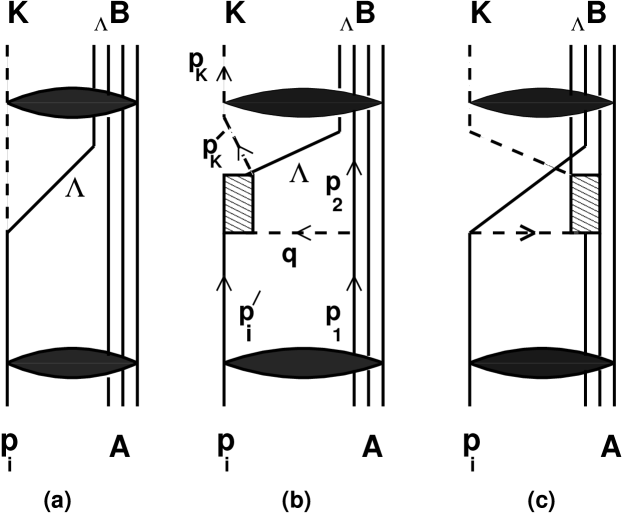
Figure 2: Graphical representation of one-nucleon (a) and two-nucleon [(b) and (c)] models. The elliptic shaded area represent the optical model interactions in the incoming and outgoing channels.

In the two-nucleon mechanism, on the other hand, the kaon production proceeds via a collision of the projectile nucleon with one of its target counterparts. This excites intermediate baryonic resonance states which decay into a kaon and a $\Lambda$ hyperon. The nucleon and the hyperon are captured into the respective nuclear orbits while the kaon rescatters into its mass shell. In this picture there are altogether three active bound state baryon wave functions taking part in the reaction process, thus allowing the large momentum transfer to be shared among three baryons. Consequently, the sensitivity of the model is shifted from high momentum parts of the bound state wave functions (not very well known) to those at relatively lower momenta where they are rather well known from $(e,e^{\prime}p)$ and $(\gamma,p)$ experiments and are relatively larger [see, e.g., [16]]. This could lead to larger cross sections. Moreover, in the TNM studies of other large momentum transfer reactions like $(p,\pi)$, $(\gamma,\pi)$, and $(\gamma,\eta)$ the distortion effects have been found to be less pronounced [17, 18].

Most of the previous calculations [10, 11, 13] of the $A(p,K^{+}){{}_{\Lambda}}B$ reaction have been done within the non-relativistic framework. However, for processes involving momentum transfers of typically 400 MeV/c or more, a non-relativistic treatment of corresponding wave functions is questionable as in this region the lower component of the Dirac spinor is no longer negligible in comparison to its upper component (see, e.g, Ref. [19]). Furthermore, in the non-relativistic description one must resolve the ambiguities of the pion-nucleon-nucleon vertex that result from the non-relativistic reduction of the full covariant pion-nucleon-nucleon vertex (see, e.g., [17, 19, 20] for more details). This is important as this vertex is used to describe the initial collision between the incoming proton and the target nucleus.

In this paper, we study the $A(p,K^{+}){{}_{\Lambda}}B$ reaction within a fully covariant TNM by retaining the field theoretical structure of the interaction vertices and by treating the baryons as Dirac particles. The initial interaction between the incoming proton and a bound nucleon of the target is described by the $\pi$, $\rho$ and $\omega$ exchange diagrams which were also used to describe the $K^{+}$ production in elementary proton-proton ($pp$) collisions [21, 22, 23]. In a previous study of the $(p,K^{+})$ reaction on a ⁴⁰Ca target [25] the latter two meson exchanges were not included. Some authors, however, have used an alternative approach for the elementary $pp\to pK^{+}\Lambda$ reaction [26, 27, 28] in which kaon exchange mechanism between the two initial state nucleons leads to the $K^{+}$ production. We have not considered this mechanism here. There are indications, from from some results reported by COSY-TOF and ANKE groups [29, 30], that the Dalitz plots for the $pp\to pK^{+}\Lambda$ reaction are dominated by the excitation of nucleon isobars, though modified by the $\Lambda p$ final state interaction (FSI) (see also Ref. [31]).

In our model, the initial state interaction of the incoming proton with a bound nucleon leads to $N^{*}$(1650)[$\frac{1}{2}^{-}$], $N^{*}$(1710)[$\frac{1}{2}^{+}$], and $N^{*}$(1720)[$\frac{3}{2}^{+}$] baryonic resonance intermediate states which make predominant contributions to elementary $pp\to pK^{+}\Lambda$ cross sections in the beam energy regime of near threshold to 10 GeV [21]. Terms corresponding to the interference among various resonance excitations are included in the total reaction amplitude. We have ignored the diagrams of type 2(a) since contributions of such processes are expected to be very small in comparison to those of the TNM.

In section II, we present the details of our formalism for calculating amplitudes corresponding to the diagrams shown in Figs. 2b and 2c, using continuum wave functions within both distorted wave (DW) and plane wave (PW) approximations. In section III, numerical results are presented for ⁴He$(p,K^{+})$${}^{5}\!\!\!_{\Lambda}$He, ¹²C$(p,K^{+})$${}^{13}\!\!\!_{\Lambda}$C, and ⁴⁰Ca$(p,K^{+})$${}^{41}\!\!\!_{\Lambda}$Ca reactions within the the PW approximation. We also give here the estimates of the effects of the initial and final state interactions which are calculated within the eikonal approximation. Summary, conclusions and future outlook of our work are given in section IV. Finally some formulas for the amplitudes are summarized in appendix A.

2 Covariant two-nucleon model for $A(p,K^{+})$ reactions

2.1 Kinematics, elementary processes and contributing diagrams

The elementary associate production reaction $pp\to pK^{+}\Lambda$ has been studied extensively both experimentally and theoretically (see, e.g., Ref. [32] for a recent review). The laboratory threshold energy for this reaction is 1.582 GeV. For the case of the $A(p,K^{+}){{}_{\Lambda}B}$ reaction the threshold energy is given by

$$E_{p}^{thres} = \frac{(m_{B}^{2}-m_{A}^{2})}{2m_{A}}+\frac{(m_{K}^{2}-m_{N}^{2})}{2m_{A}}+\frac{m_{B}m_{K}}{m_{A}}-m_{N},$$ (1)

where $m_{B}$ and $m_{A}$ are the masses of the hypernucleus ${}_{\Lambda}B$ and the target nucleus A, respectively and $m_{K}$ is the mass of the kaon. $E_{p}^{thres}$ is 0.739 GeV and 0.602 GeV for ¹²C and ⁴⁰Ca targets, respectively which are considerably lower than the threshold energy value of the elementary production process as stated above.

The $(p,K^{+})$ reaction is characterized by the momentum transfer ${\bf p}_{cm}={\bf p}_{i}-{\bf p}_{K}$ to the residual nucleus. In Fig. 1, ${p}_{cm}$ are plotted as a function of the laboratory beam energy for several values of the outgoing kaon angles for ¹²C and ⁴⁰Ca targets. It is clear that $p_{cm}$ varies between 1 GeV to 5 GeV. In the ONM a single nucleon alone carries this huge momentum to the nucleus. In the PW approximation, the ONM cross section of the $(p,K^{+})$ reaction is directly proportional to the modulus square of the bound state wave functions in the momentum space. Since at these large momenta the magnitudes of the bound state wave functions are very small, the corresponding cross sections are quite weak. Of course, the inclusion of the distortions changes this model towards a multi-nucleon mechanism thus shifting the sensitivity of the model to lower momentum components of the bound state wave functions. Therefore, apriori, these effects are very important in the ONM description of such reactions.

The data on the associate production reaction $pp\to p\Lambda K^{+}$, are available for beam energies ranging from very close to the threshold to upto 10 GeV which can be well described within an effective Lagrangian approach [21, 22, 23]. In this model, the associated kaon production proceeds via excitation, propagation and decay of the $N^{*}$(1650), $N^{*}$(1710) and $N^{*}$(1720) intermediate baryonic resonant states, in the initial collision of two nucleons in the incident channel. The coupling constants at the nucleon-nucleon-meson vertices are fixed by fitting to an elastic $NN$ $T$ matrix while those at resonance-nucleon-meson vertices are determined from the experimental branching ratios for the decay of the resonance into relevant channels except for those involving the $\omega$ meson where they are determined from the vector meson dominance (VMD) hypothesis. To describe the near threshold data

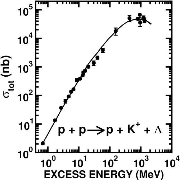
Figure 3: Comparison of the calculated total cross sections for the $p+p\rightarrow p+K^{+}+\Lambda$ reaction with the corresponding experimental data [taken from Refs. [33, 34]] as a function of the excess energy. The calculated cross sections represent the coherent sum of the amplitudes corresponding to all the contributing baryonic resonant states and the meson exchange processes.

the FSI effects in the final channel are included within the framework of the Watson-Migdal theory. As an example, we show in Fig. 3 a comparison of calculated and experimental total cross sections for the $pp\to pK^{+}\Lambda$ reaction. The FSI amplitude has been calculated using the scattering length and the effective range parameters of the model $\tilde{A}$ of $\Lambda-p$ interaction described in Ref. [24]. The cross sections are plotted as a function of the excess energy (defined as $\sqrt{s}-m_{N}-m_{K^{+}}-m_{\Lambda}$, where $\sqrt{s}$ is the invariant mass). It is clear that the model provides a good description of the experimental data in the entire range of beam energies. While at near threshold beam energies the reaction proceeds predominantly via excitation of the $N^{*}$(1650) resonance, the other resonances become more and more important with increasing beam energies. One pion exchange graphs dominate the production process for all the energies.

The structure of our TNM for the $(p,K^{+})$ reaction is similar to that of the effective Lagrangian approach described above. The initial interaction between the incoming proton and a bound nucleon of the target is described not only by the dominant one-pion exchange mechanism but also by the $\rho$ and $\omega$ exchange processes. The latter may become more important at backward angles of the outgoing $K^{+}$ spectrum where momentum transfers are relatively larger. We use the same effective Lagrangians and vertex parameters to model these interactions. The initial state interaction between the two nucleons leads to the $N^{*}(1650)[\frac{1}{2}^{-}]$, $N^{*}(1710)[\frac{1}{2}^{+}]$, and $N^{*}(1720)[\frac{3}{2}^{+}]$ baryonic resonance intermediate states. The vertex parameters here too are the same as those used in the description of the elementary reaction. Terms corresponding to the interference between various amplitudes are retained.

We denote the diagrams (and the corresponding amplitudes) by ”projectile emission (PE)” if the intermediate meson starts from the projectile and rescatters from the target nucleon which is excited to an intermediate baryonic resonance state [Fig. 2(c)] and by ”target emission” if the opposite is the case [Fig. 2(b)]. In the two amplitudes there is a tremendous variation in the energy of the intermediate meson. For example, in Fig. 2(b), the energy of the exchanged meson is given by the difference between single-particle binding energies of the initial and final intermediate states which is very small and can be approximated to zero. On the other hand, in Fig. 2(c), the energy of the intermediate meson is almost equal to the incident proton energy. Due to different four momentum transfers the behavior of the two amplitudes is quite different and they explore different regions of the intermediate meson propagator. Thus corresponding medium effects have to be known over a wide range of energy and momenta in order to incorporate their effects into the calculations.

2.2 Calculations of the TNM amplitudes

The effective Lagrangian for the nucleon-nucleon-meson vertices are given by

$${\mathscr{L}}_{NN\pi} = -\frac{g_{NN\pi}}{2m_{N}}{\bar{\Psi}}\gamma_{5}{\gamma}_{\mu}\mbox{\boldmath$\tau$}\cdot(\partial^{\mu}{\bf\Phi}_{\pi})\Psi.$$ (2)

$${\mathscr{L}}_{NN\rho} = -g_{NN\rho}\bar{\Psi}_{N}\left(\gamma_{\mu}+\frac{k_{\rho}}{2m_{N}}\sigma_{\mu\nu}\partial^{\nu}\right)\mbox{\boldmath$\tau$}\cdot\mbox{\boldmath$\rho$}^{\mu}\Psi_{N}.$$ (3)

$${\mathscr{L}}_{NN\omega} = -g_{NN\omega}\bar{\Psi}_{N}\left(\gamma_{\mu}+\frac{k_{\omega}}{2m_{N}}\sigma_{\mu\nu}\partial^{\nu}\right)\omega^{\mu}\Psi_{N}.$$ (4)

We have used notations and conventions of Bjorken and Drell [35]. In Eq. (2) $m_{N}$ denotes the nucleon mass. In Eqs. (3) - (4) $\sigma_{\mu\nu}$ is defined as

$$\sigma_{\mu\nu} = {i\over 2}(\gamma_{\mu}\gamma_{\nu}-\gamma_{\nu}\gamma_{\mu})$$ (5)

The $NN$-meson vertices are corrected for off-shell effects by multiplying the corresponding coupling constants by form factors of the forms [21]

$$F_{i}^{NN} = \left(\frac{\lambda_{i}^{2}-m_{i}^{2}}{\lambda_{i}^{2}-q_{i}^{2}}\right),$$ (6)

where $q_{i}$ and $m_{i}$ are the four momentum and mass of the $i$th exchanged meson and $\lambda_{i}$ are the corresponding cutoff parameters [their values are taken to be the same as those given in Ref. [21]]. The latter governs the range of the suppression of the contributions of high momenta.

As the $\Lambda$-hyperon has zero isospin, only isospin-1/2 nucleon resonances are allowed. Below 2 GeV center of mass (c.m.) energy, only three resonances, $N^{*}$(1650), $N^{*}$(1710), and $N^{*}$(1720), have significant decay branching ratios into the $K^{+}\Lambda$ channel. As in the description of the associate $K^{+}$ production in the elementary $pp$ collisions, only these three resonances have been considered in this work. The effective Lagrangians for the resonance-nucleon-meson vertices are written as [21, 36, 37, 38, 39]

$${\mathscr{L}}_{N_{1/2}^{*}N\pi} = -g_{N_{1/2}^{*}N\pi}{\bar{\Psi}}_{N_{1/2}^{*}}i{\Gamma}\mbox{\boldmath$\tau$}{\bf\Phi}_{\pi}\Psi+{\rm h.c.},$$ (7)

$${\mathscr{L}}_{N_{1/2}^{*}N\rho} = -g_{N_{1/2}^{*}N\rho}\bar{\Psi}_{N^{*}}\frac{1}{2m_{N}}\Gamma_{\mu\nu}\partial^{\nu}\mbox{\boldmath$\tau$}\cdot\mbox{\boldmath$\rho$}^{\mu}\Psi_{N}.+{\rm h.c.}$$ (8)

$${\mathscr{L}}_{N_{1/2}^{*}N\omega} = -g_{N_{1/2}^{*}N\omega}\bar{\Psi}_{N^{*}}\frac{1}{2m_{N}}\Gamma_{\mu\nu}\partial^{\nu}\omega^{\mu}\Psi_{N}.+{\rm h.c.}$$ (9)

$${\mathscr{L}}_{N_{3/2}^{*}N\pi} = \frac{g_{N_{3/2}^{*}N\pi}}{m_{\pi}}{\bar{\Psi}}_{\mu}^{N^{*}}\Gamma_{\pi}{\mbox{\boldmath$\tau$}}\cdot\partial^{\mu}{\bf\Phi}_{\pi}\Psi+{\rm h.c.}.$$ (10)

$${\mathscr{L}}_{N_{3/2}^{*}N\rho} = {\rm i}\frac{g_{N_{3/2}^{*}N\rho}}{m_{N^{*}}+m_{N}}{\bar{\Psi}}_{\mu}\mbox{\boldmath$\tau$}\left(\partial^{\nu}\mbox{\boldmath$\rho$}^{\mu}-\partial^{\mu}\mbox{\boldmath$\rho$}^{\nu}\right)\gamma_{\nu}{\gamma_{5}}\Psi_{N}+{\rm h.c.}.$$ (11)

$${\mathscr{L}}_{N_{3/2}^{*}N\omega} = {\rm i}\frac{g_{N_{3/2}^{*}N\omega}}{m_{N^{*}}+m_{N}}{\bar{\Psi}}_{\mu}\mbox{\boldmath$\tau$}\left(\partial^{\nu}\omega^{\mu}-\partial^{\mu}\omega^{\nu}\right)\gamma_{\nu}{\gamma_{5}}\Psi_{N}+{\rm h.c.}.$$ (12)

The operator $\Gamma(\Gamma_{\pi})$ is either $\gamma_{5}$ (unity) or unity $(\gamma_{5})$ depending on whether the parity of the resonance is even or odd, respectively. The operator $\Gamma_{\mu\nu}$ is $\sigma_{\mu\nu}$ or $\gamma_{5}\sigma_{\mu\nu}$ for these two cases. ${\bar{\Psi}}_{\mu}$ is the $N^{*}$(1720) vector spinor. It may be noted that we have used the conventional Rarita-Swinger coupling for the spin-$\frac{3}{2}$ particle [36, 37] which also has off-shell contributions to the spin-$\frac{1}{2}$ partial waves. To describe the latter, an operator $\Theta_{\alpha\mu}(z)=g_{\alpha\nu}-\frac{1}{2}(1+2z)\gamma_{\alpha}\gamma_{\mu}$ has also been included in the vector spinor vertex [36, 38, 39, 40]. The choice of the off-shell parameter $z$ is arbitrary; it is treated as a free parameter to be determined by fitting to the data. In Ref. [41] an alternative interaction has been suggested that does not activate the spurious spin-$\frac{1}{2}$ degree of freedom. We, however, work with the Lagrangians as given in Eqs. (10)-(12). It may further be noted that we have used a pseudovector (PV) coupling for the $NN\pi$ vertex and a pseudoscalar (PS) one for $N_{1/2}^{*}N\pi$ and $N_{1/2}^{*}\Lambda K$ vertices. This provides the best description of the $pp\to p\Lambda K^{+}$ data [21].

The effective Lagrangians for the resonance-hyperon-kaon vertices are written as

$${\mathscr{L}}_{N_{1/2}^{*}\Lambda K^{+}} = -g_{N^{*}_{1/2}\Lambda K^{+}}{\bar{\Psi}}_{N^{*}}{i\Gamma}\mbox{\boldmath$\tau$}{\bf\Phi}_{K^{+}}\Psi+{\rm h.c.}.$$ (13)

$${\mathscr{L}}_{N_{3/2}^{*}\Lambda K^{+}} = \frac{g_{N^{*}_{3/2}\Lambda K^{+}}}{m_{K^{+}}}{\bar{\Psi}}_{\mu}^{N^{*}}\Gamma_{\pi}{\mbox{\boldmath$\tau$}}\cdot\partial^{\mu}{\bf\Phi}_{K^{+}}\Psi+{\rm h.c.}.$$ (14)

Signs and values of various coupling constants have been taken from [21, 25] and are shown in Table 1. It should be noted that for the nucleon-nucleon-meson vertices, the coupling constants were taken to be energy dependent in the same way as that described in Ref. [21]. The $N_{1/2}^{*}N$-meson and $N_{3/2}^{*}N$-meson vertices are corrected for the off-shell effects by multiplying the corresponding coupling constants by form factors of the forms (which is also used in Ref. [42]).

$$F_{j}^{NN^{*}} = \left[\frac{(\lambda_{i}^{N^{*}})^{4}}{(\lambda_{j}^{N^{*}})^{4}+(q_{j}^{2}-m_{j}^{2})^{2}}\right],j=\pi,\rho,\omega$$ (15)

The values of the cut-off parameters appearing therein are taken to be 1.2 GeV in all the cases in order to reduce the number of free parameters. It may noted that same form of $F_{j}^{NN^{*}}$ and the value of the cut-off parameter was also used in the calculations of the elementary cross sections shown in Fig. 3.

After having established the effective Lagrangians and the coupling constants, one can write down, by following the well known

Table 1: Coupling constants for various vertices used in the calculations.

Vertex	Coupling Constant($g$)
$NN\pi$	12.56
$NN\rho$	2.00
$NN\omega$	24.05
$N^{*}(1710)N\pi$	1.04
$N^{*}(1710)N\rho$	4.14
$N^{*}(1710)N\omega$	1.22
$N^{*}(1710)\Lambda K^{+}$	6.12
$N^{*}(1650)N\pi$	0.81
$N^{*}(1650)N\rho$	2.62
$N^{*}(1650)N\omega$	1.80
$N^{*}(1650)\Lambda K^{+}$	0.76
$N^{*}(1720)N\pi$	0.21
$N^{*}(1720)N\rho$	33.75
$N^{*}(1720)N\omega$	16.93
$N^{*}(1720)\Lambda K^{+}$	0.87

Feynman rules, the amplitudes for graphs 2(b) and 2(c). The isospin part is treated separately which gives rise to a constant factor for each graph. For example, the amplitude for graph 2(b) with one-pion exchange mechanism and excitation of the positive parity spin-${1\over 2}$ baryonic resonance is given by,

$$M_{2b}(N^{*}_{1/2}) = C_{iso}^{2b}\biggl{(}\frac{g_{NN\pi}}{2m_{N}}\biggr{)}(g_{N_{1/2}^{*}N\pi})(g_{N^{*}_{1/2}\Lambda K^{+}}){\bar{\psi}}(p_{2})\gamma_{5}\gamma_{\mu}q^{\mu}$$ (16)

$$\times \psi(p_{1})D_{\pi}(q){\bar{\psi}}(p_{\Lambda})\gamma_{5}D_{N^{*}_{1/2}}(p_{N^{*}})\gamma_{5}$$

$$\times \Phi^{(-)*}_{K}(p_{K}^{\prime},p_{K})\Psi^{(+)}_{i}(p_{i}^{\prime},p_{i}),$$

where various momenta are as defined in Fig. 2(b). In addition, $p_{N^{*}}$ is the momentum associated with the intermediate resonance and $p_{\Lambda}$ is that associated with the $\Lambda$ hyperon. The isospin factor $C_{iso}^{2b}$ is unity. For the graph 2(c) also it is unity. The functions $\psi$ are the four component (spin space) Dirac spinor in momentum space [19, 43]. $\Phi_{K}^{(-)*}(p_{K}^{\prime},p_{K})$ [$\Psi_{i}^{(+)}(p_{i}^{\prime},p_{i})$] is the wave function for the outgoing kaon [incoming proton] with appropriate boundary conditions. Function $D_{i}(p_{i})$ is the propagator for the $i$th particle with momentum $p_{i}$. The propagators for mesons and spin-${1\over 2}$ and spin-${3\over 2}$ intermediate resonances are given by

$$D_{\pi}(q) = {i\over{q^{2}-m_{\pi}^{2}-\Pi_{\pi}(q)}},$$ (17)

$$D_{\rho}^{\mu\nu}(q) = -i\left({g^{\mu\nu}-q^{\mu}q^{\nu}/q^{2}}\over{q^{2}-m_{\rho}^{2}-\Pi_{\rho}(q)}\right),$$ (18)

$$D_{N^{*}_{1/2}}(p) = i\left[{p_{\eta}\gamma^{\eta}+m_{N^{*}_{1/2}}}\over{p^{2}-(m_{N^{*}_{1/2}}-i\Gamma_{N^{*}_{1/2}}/2)^{2}}\right],$$ (19)

$$D_{N^{*}_{3/2}}^{\mu\nu}(p) = -\frac{i(p\!\!\!/+m_{N^{*}_{3/2}})}{p^{2}-(m_{N^{*}_{3/2}}-i\Gamma_{N^{*}_{3/2}}/2)^{2}}$$ (20)

$$\times[g^{\mu\nu}-\frac{1}{3}\gamma^{\mu}\gamma^{\nu}-\frac{2}{3m_{N^{*}_{3/2}}^{2}}p^{\mu}p^{\nu}+\frac{1}{3m_{N^{*}_{3/2}}^{2}}(p^{\mu}\gamma^{\nu}-p^{\nu}\gamma^{\mu})].$$

In Eq. (17) $\Pi_{\pi}(q)$ is the (complex) pion self energy which accounts for the medium effects on the propagation of the pion in the nucleus. Similarly, $\Pi_{\rho}(q)$, in Eq. (18) is the same for the $\rho$ meson. We have adopted the approach of Ref. [44] for the calculation of $\Pi_{\pi}(q)$ which has been renormalized by including the short-range repulsion effects through the constant Landau-Migdal parameter $g^{\prime}$. All the relevant formulas for this calculation are given in Ref. [19]. Like $(p,\pi)$ [19] and $(p,p^{\prime}\pi)$ [45] reactions, $(p,K^{+})$ cross sections too are sensitive to the parameter $g^{\prime}$ [25]. For the self energies of $\rho$ and $\omega$ mesons, we have followed the procedure described in Ref. [46].

In Eqs. (19) and (20), $\Gamma_{N^{*}}$ is the total width of the resonance which is introduced in the denominator term to account for the finite life time of the resonances for decays into various channels. $\Gamma_{N^{*}}$ is a function of the center of mass momentum of the decay channel, and it is taken to be the sum of the widths for pion and rho decay (the other decay channels are considered only implicitly by adding their branching ratios to that of the pion channel) [21]. The medium corrections on the intermediate resonance widths have not been included. We do not expect any major change in our results due to these effects. As is pointed out in [47, 48, 49], the medium correction effects on widths of the $s$- and $p$-wave resonances, which make the dominant contribution to the cross sections being investigated here, are not substantial. On the other hand, any medium modification in the width of the $d$-wave resonance is unlikely to alter our results as their contributions to the cross sections are negligible [46].

The four component Dirac spinors $\psi(p_{j})$ are the solutions of the Dirac equation in momentum space for a bound state problem in the presence of an external potential field [19, 50]

$$p\!\!\!/\psi(p) = m_{N}\psi(p)+F(p),$$ (21)

where

$$F(p) = \delta(p_{0}-E)\Biggl{[}\int d^{3}p^{\prime}V_{s}(-{\bf p}^{\prime})\psi({\bf p}+{\bf p}^{\prime})$$ (22)

$$- \gamma_{0}\int d^{3}p^{\prime}V_{v}^{0}(-{\bf p}^{\prime})\psi({\bf p}+{\bf p}^{\prime})\Biggr{]}.$$

In our notation ’$p$’ represents a four momentum, and ’${\bf p}$’ a three momentum. The magnitude of ${\bf p}$ ($|p|$) is represented by $k$, and its directions by ${\hat{p}}$. ’$p_{0}$’ represents the time-like component of the momentum. Similarly, the magnitude and directions of the radial vector ${\bf r}$ is represented by $a$ and ${\hat{r}}$, respectively. In Eq. (22), $V_{s}$ and $V_{v}^{0}$ represent a scalar potential and time-like component of a vector potential in the momentum space. The spinors $\psi(p)$ and $F(p)$ are written as

$$\psi(p) = \delta(p_{0}-E){{f(k){\mathscr{Y}}_{\ell 1/2j}^{m_{j}}(\hat{p})}\choose{-ig(k){\mathscr{Y}}_{\ell^{\prime}1/2j}^{m_{j}}(\hat{p})}},$$

$$F(p) = \delta(p_{0}-E){{\zeta(k){\mathscr{Y}}_{\ell 1/2j}^{m_{j}}(\hat{p})}\choose{-i\zeta^{\prime}(k){\mathscr{Y}}_{\ell^{\prime}1/2j}^{m_{j}}(\hat{p})}},$$ (23)

where $f(k)$[$\zeta(k)$] is the radial part of the upper component of the spinor $\psi(p)$[$F(p)$]. Similarly $g(k)$[$\zeta^{\prime}(k)$] are the same of their lower component. Functions $f(p)$ and $g(p)$ are the Fourier transforms of the radial parts of the corresponding coordinate space spinors. $\zeta(k)$s are related to $f$, $g$ and the scalar and vector potentials in the following way

$$\zeta(k) = \zeta_{s}(k)-\zeta_{v}(k),$$

$$\zeta^{\prime}(k) = \zeta^{\prime}_{s}(k)-\zeta^{\prime}_{v}(k),$$ (24)

where

$$\zeta_{s}(k) = 4\pi\int dk^{\prime}k^{\prime 2}V_{s}(k^{\prime})\frac{f(k+k^{\prime})}{(1+k/k^{\prime})^{\ell}},$$ (25)

$$\zeta_{v}(k) = 4\pi\int dk^{\prime}k^{\prime 2}V_{v}^{0}(k^{\prime})\frac{f(k+k^{\prime})}{(1+k/k^{\prime})^{\ell}},$$ (26)

$$\zeta_{s}^{\prime}(k) = 4\pi\int dk^{\prime}k^{\prime 2}V_{s}(k^{\prime})\frac{g(k+k^{\prime})}{(1+k/k^{\prime})^{\ell^{\prime}}},$$ (27)

$$\zeta_{v}^{\prime}(k) = 4\pi\int dk^{\prime}k^{\prime 2}V_{v}^{0}(k^{\prime})\frac{g(k+k^{\prime})}{(1+k/k^{\prime})^{\ell^{\prime}}}.$$ (28)

More details of the derivations Eqs. (21)-(28) can be found in appendix A of the Ref. [19]. In Eq. (23), ${\mathscr{Y}}_{\ell 1/2j}^{m_{j}}$ are the coupled spherical harmonics

$${\mathscr{Y}}_{\ell 1/2j}^{m_{j}} = <\ell m_{\ell}1/2\mu_{i}|jm_{j}>Y_{\ell m_{\ell}}(\hat{p})\chi_{1/2\mu_{i}},$$ (29)

where $\ell^{\prime}=2\ell-j$ with $\ell$ and $j$ being the orbital and total angular momenta, respectively and $Y$ represents the spherical harmonics. $\chi_{1/2\mu_{i}}$ is the spin space wave function of a spin-$\frac{1}{2}$ particle. In this paper we consider only those cases where the final state has a pure single particle configuration. Likewise, the intermediate states are supposed to have pure single-hole or particle structures.

The incident proton spinor and the outgoing kaon field are given by

$$\Psi_{i}^{(+)}(p^{\prime}_{i},p_{i}) = \delta(p^{\prime}_{i0}-E_{i})\sum_{J_{p}L_{p}M_{p}}<L_{p}M_{p}-\mu 1/2\mu|J_{p}M_{p}>Y^{*}_{L_{p}M_{p}-\mu}(\hat{p_{i}})$$ (30)

$$\times {{F_{L_{p}J_{p}}(k^{\prime}_{i},k_{i}){\mathscr{Y}}_{L_{p}1/2J_{p}}^{M_{p}}({\hat{p}}^{\prime}_{i})}\choose{G_{L^{\prime}_{p}J_{p}}(k^{\prime}_{i},k_{i}){\mathscr{Y}}_{L^{\prime}_{p}1/2J_{p}}^{M_{p}}({\hat{p}}^{\prime}_{i})}},$$

$$\Phi_{K}^{(-)*}(p_{K}^{\prime},p_{K}) = \delta(p^{\prime}_{K0}-E_{K})\sum_{\ell_{K}m_{K}}(-)^{\ell_{K}}Y_{\ell_{K}m_{K}}({\hat{p}}_{K})Y_{\ell_{K}m_{K}}^{*}({\hat{p}}^{\prime}_{K})$$ (31)

$$\times f_{\ell_{K}}(k^{\prime}_{K},k_{K}),$$

where $E_{i}$ and $E_{K}$ represents the energies of the incident proton and out going kaon, respectively, and where we have defined

$$F_{L_{p}J_{p}}(k^{\prime}_{i},k_{i}) = \frac{1}{2\pi^{2}}\int_{0}^{\infty}j_{L_{p}}(k^{\prime}_{i}a)\,F^{C}_{L_{p}J_{p}}(k_{i},a)a^{2}da,$$ (32)

$$G_{L^{\prime}_{p}J_{p}}(k^{\prime}_{i},k_{i}) = \frac{1}{2\pi^{2}}\int_{0}^{\infty}j_{L^{\prime}_{p}}(k^{\prime}_{i}a)\,G^{C}_{L^{\prime}_{p}J_{p}}(k_{i},a)a^{2}da,$$ (33)

$$f_{\ell_{K}}(k^{\prime}_{K},k_{K}) = \frac{1}{2\pi^{2}}\int_{0}^{\infty}j_{\ell_{K}}(k^{\prime}_{K}a)\,f^{C}_{\ell_{k}}(k_{K},a)a^{2}da.$$ (34)

In Eqs. (32) and (33), $F^{C}_{L_{p}J_{p}}$ and $G^{C}_{L^{\prime}_{p}J_{p}}$ are the coordinate space spinors which are obtained by solving the Dirac equation for the scattering state with appropriate complex scalar and vector potentials. In Eqs. (30)-(35), the momentum arguments $p$ denote the quantum numbers of the asymptotic free states whereas $p^{\prime}$ represent the momentum coordinates. A short derivation of Eqs. (30)-(31) is presented in appendix B. In Eq. (34) wave function $f^{C}_{\ell_{K}}$ is the coordinate space solution of the Klein-Gordon equation with kaon-nucleus optical potential (see, e.g., Ref [51]). In these equations $j_{\ell}$ represent the spherical Bessel function. It should be mentioned here that due to oscillatory nature of the asymptotic these wave functions in the asymptotic region, the integrals involved in Eqs. (32)-(34) converge poorly. Such integrals can, however, be calculated very accurately by using a contour integration method [52].

In the PW approximation, the wave functions $\Psi_{i}^{(+)}(p^{\prime}_{i},p_{i})$ and $\Phi_{K}^{(-)*}(p_{K}^{\prime},p_{K})$ are given by

$$\Psi_{i}^{(+)}(p^{\prime}_{i},p_{i}) = \sqrt{\frac{E_{i}+m_{N}}{2m_{N}}}{{\chi_{\mu_{i}}}\choose\frac{\sigma\cdot p}{E_{i}+m_{N}}\chi_{\mu_{i}}}\delta^{4}(p^{\prime}_{i}-p_{i}),$$ (35)

$$\Phi_{K}^{(-)*}(p_{K}^{\prime},p_{K}) = \delta^{4}(p^{\prime}_{K}-p_{K}).$$ (36)

In Eq. (35) $\chi_{\mu_{i}}$ represents the two component Pauli spinor. The other symbols have the same meaning as in Ref. [35].

By repeated use of Eqs. (21) and (22) one can perform the tedious but straight forward algebra to trace out the $\gamma$ matrices from the expression for the amplitudes [e.g., Eq. (16)]. Furthermore, by using Eqs. (21)-(28) and (30)-(33) and performing the angular momentum algebra one can get the amplitudes in a form which is suitable for numerical evaluation. We write in appendix A, e.g., the final form of the amplitude $M_{2b}$ [Eq. (16)] in both full distorted wave as well as plane wave approximations.

To get the $T$ matrix of the $(p,K^{+})$ reaction, one has to integrate the amplitude corresponding to each graph over all the independent intermediate momenta subject to constraints imposed by the momentum conservation at each vertex. For instance, for the amplitude corresponding to Eq. (16) the respective $T$ matrix is given by

$$T_{2b}(N^{*}_{1/2}) = \int\frac{d^{4}p^{\prime}_{i}}{(2\pi)^{4}}\int\frac{d^{4}p^{\prime}_{K}}{(2\pi)^{4}}\int\frac{d^{4}p_{\Lambda}}{(2\pi)^{4}}\int\frac{d^{4}p_{2}}{(2\pi)^{4}}$$ (37)

$$\times \delta(q-p_{1}+p_{2})\delta(p_{N^{*}}-p_{K}-p_{\Lambda})$$

$$\times \delta(p_{\Lambda}-p_{i}^{\prime}-q+p_{K}^{\prime})M_{2b}(N^{*}_{1/2}).$$

It can be seen, from Eq. (37), that in the full distorted wave theory one would be required to perform a twelve dimensional integration to evaluate the $T$-matrix $T_{2b}$ which requires a tremendous numerical effort. This gets further complicated due to the fact that the number of partial waves required in Eqs. (30)-(32) are quite large for these high energy reactions. On the other hand, in the plane wave approximation the integrations over variables $p_{i}^{\prime}$ and $p_{K}^{\prime}$ become redundant. This not only reduces the dimensionality of the integrations by a factor of 2 but also removes the requirement of partial wave summations altogether. In this exploratory study we would like to make calculations for very many cases involving a variety of targets and beam energies in order to understand the basic mechanism of this reaction and to get the estimates of the order of magnitudes of various cross sections to guide the planning of the future experiments. We have, therefore, made our calculations in a numerically simpler plane wave theory. However, estimates of the distortions have been made within the eikonal approximation.

The differential cross section for the $(p,K^{+})$ reaction is given by

$$\frac{d\sigma}{d\Omega} = \frac{1}{(4\pi)^{2}}\frac{m_{p}m_{A}m_{B}}{(E_{p_{i}}+E_{A})^{2}}\frac{p_{K}}{p_{i}}\sum_{m_{i}m_{f}}|T_{m_{i}m_{f}}|^{2},$$ (38)

where $E_{p_{i}}$ and $E_{A}$ are the total energies of incident proton and the target nucleus, respectively while $m_{p}$, $m_{A}$ and $m_{B}$ are the masses of the proton, and the target and residual nuclei, respectively. The summation is carried out over initial ($m_{i}$) and final ($m_{f}$) spin states. $T$ is the final $T$ matrix obtained by summing the transition matrices corresponding to all the graphs.

3 Results and Discussions

3.1 The nuclear and hypernuclear structure and bound state spinors

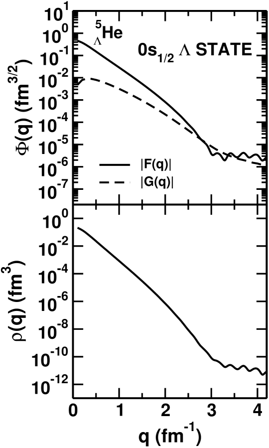
Figure 4: (Upper panel) Momentum space spinors [$\Phi(q)$] for $0s_{1/2}$ $\Lambda$ orbit in ${}^{5}\!\!\!_{\Lambda}$He hypernucleus. $|F(q)|$ and $|G(q)|$ are the upper and lower components of the spinor, respectively. (Lower panel) Momentum distribution [$\rho(q)=|F(q)|^{2}+|G(q)|^{2}$] for the same hyperon state calculated with these wave functions.

The spinors for the final bound hypernuclear state (corresponding to momentum $p_{\Lambda}$) and for two intermediate nucleonic states (corresponding to momenta $p_{1}$ and $p_{2}$) are required to perform numerical calculations of various amplitudes. We assume these states to be of pure-single particle or single-hole configurations with the core remaining inert. To simplify the nuclear structure problem the quantum numbers of the two intermediate states are taken to be the same although it is straight forward to include also those cases where they may occupy different orbits. The spinors in the momentum space are obtained by Fourier transformation of the corresponding coordinate space spinors which are the solutions of the Dirac equation with potential fields consisting of an attractive scalar part ($V_{s}$) and a repulsive vector part ($V_{v}$) having a Woods-Saxon form. This choice appears justified as the Dirac Hartree-Fock calculations [53, 54] suggest that these potentials tend to follow the nuclear shape. The same potential form has also been used in the relativistic ONM [15] and TNM calculations [19] of the $(p,\pi)$ reaction.

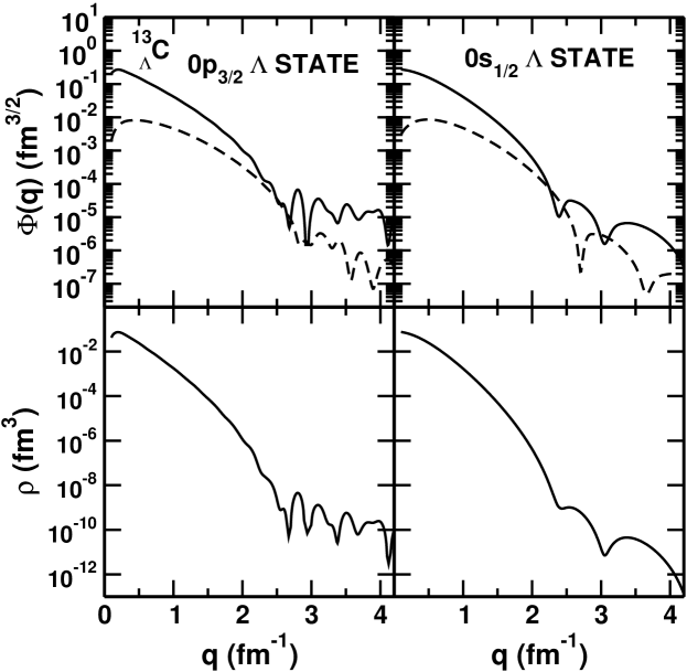
Figure 5: same as in Fig. 4 for $0p_{3/2}$ $\Lambda$ and $0s_{1/2}$ $\Lambda$ orbits in ${}^{13}\!\!\!_{\Lambda}$C hypernucleus.

With a fixed set of the geometry parameters (reduced radii $r_{s}$ and $r_{v}$ and diffusenesses $a_{s}$ and $a_{v}$), the depths of the potentials were searched in order to reproduce the binding energies of the particular state (the corresponding values are given in Table 2). We use the same geometry for the scalar and vector potentials. The depths of potentials $V_{s}$ and $V_{v}$ were further constrained by requiring that their ratios are equal to -0.81 as suggested in Ref. [55]. Experimental inputs have been used for the configurations and the single baryon binding energies of the states in hypernuclei ⁵$\!\!\!{}_{\Lambda}$He [2] and ¹³$\!\!\!{}_{\Lambda}$C [2, 3]. However, the quantum numbers as well as the single baryon binding energies for states in ⁴¹$\!\!\!{}_{\Lambda}$C hypernucleus have been taken from the density dependent relativistic hadron field (DDRH) theory predictions of Ref. [7], which reproduce the corresponding experimental binding energies reasonably well. In this case, we have compared, for each state, the spinors calculated by our well-depth search method with those calculated within the DDRH [7] theory and find an excellent agreement between the two.

Table 2: Searched depths of vector and scalar potentials and the binding energies of the $\Lambda$ and nucleon bound states.

State	Binding Energy ($\epsilon$)	$V_{v}$	$r_{v}$	$a_{v}$	$V_{s}$	$r_{s}$	$a_{s}$
	(MeV)	(MeV)	(fm)	(fm)	(MeV)	(fm)	(fm)
${}^{5}\!\!\!_{\Lambda}$He$(0s_{1/2})$	3.12	135.424	0.983	0.578	-167.190	0.983	0.606
4He$(0s_{1/2})$	19.814	384.053	0.983	0.578	-429.695	0.983	0.606
${}^{13}\!\!\!_{\Lambda}$C$(0p_{3/2})$	0.860	180.712	0.983	0.578	-223.101	0.983	0.606
${}^{13}\!\!\!_{\Lambda}$C$(0p_{1/2})$	0.708	206.161	0.983	0.578	-254.520	0.983	0.606
${}^{13}\!\!\!_{\Lambda}$C$(0s_{1/2})$	11.690	166.473	0.983	0.578	-205.522	0.983	0.606
12C$(0p_{3/2})$	15.957	382.598	0.983	0.578	-472.343	0.983	0.606
${}^{41}\!\!\!_{\Lambda}$Ca$(0s_{1/2})$	17.882	154.884	0.987	0.676	-191.215	0.982	0.700
${}^{41}\!\!\!_{\Lambda}$Ca$(0p_{3/2})$	9.677	179.485	0.987	0.676	-221.587	0.982	0.700
${}^{41}\!\!\!_{\Lambda}$Ca$(0p_{1/2})$	9.140	188.188	0.987	0.676	-232.331	0.982	0.700
${}^{41}\!\!\!_{\Lambda}$Ca$(0d_{5/2})$	1.544	207.490	0.987	0.676	-256.160	0.982	0.700
${}^{41}\!\!\!_{\Lambda}$Ca$(1s_{1/2})$	1.108	192.044	0.987	0.676	-237.091	0.982	0.700
${}^{41}\!\!\!_{\Lambda}$Ca$(0d_{3/2})$	0.753	230.206	0.987	0.676	-284.205	0.982	0.700
40Ca$(0d_{3/2})$	8.333	360.980	0.987	0.676	-445.660	0.982	0.700

In Figs. (4)-(6) we show the lower and upper components of the Dirac spinors in momentum space for the $0s_{1/2}$ hyperon in ${}^{5}\!\!\!_{\Lambda}$He, $0p_{3/2}$ and $0s_{1/2}$ hyperons in ${}^{13}\!\!\!_{\Lambda}$C, and $0d_{3/2}$ and $0p_{1/2}$ hyperons in ${}^{41}\!\!\!_{\Lambda}$Ca, respectively. In each case, we note that only for momenta $<$ 1.5 fm^-1, is the lower component of the spinor substantially smaller than the upper component. In the region of momentum transfer pertinent to exclusive kaon production in proton-nucleus collisions, the lower components of the spinors are not negligible as compared to the upper component which clearly demonstrates that a fully relativistic approach is essential for an accurate description of this reaction.

The spinors calculated in this way provide a good description of the experimental nucleon momentum distributions for various nucleon orbits as is shown in Ref. [19]. In the lower panel of each of Figs. (4)-(6), we show momentum distribution $\rho(q)\,[=F(q)|^{2}+|G(q)|^{2}]$ [16] of the corresponding $\Lambda$ hyperon. It can be noted that in each case the momentum density of the hyperon shell, in the momentum region around 0.35 GeV/c, is at least 2-3 orders of magnitude larger that around 1.0 GeV/c. Since, in the TNM the large momentum is shared among three baryons, the model is sensitive to the bound state spinors in the momentum regime where they are well described and are quite large. Therefore, one expects to get a larger cross section for exclusive meson production reactions within this model.

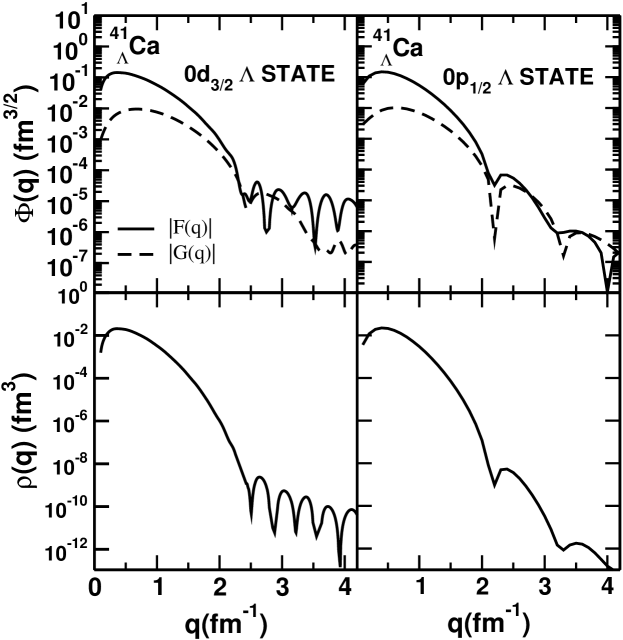
Figure 6: Same as in Fig. 4 for $0d_{3/2}$ $\Lambda$ and $0p_{1/2}$ $\Lambda$ orbits in ${}^{41}\!\!\!_{\Lambda}$Ca hypernucleus.

3.2 Cross sections for A($p,K^{+})_{\Lambda}$B reaction

3.2.1 Results within the plane wave approximation

The self-energies $\Pi_{\pi}$, $\Pi_{\rho}$ and $\Pi_{\omega}$ of pion, rho and omega mesons, respectively, are another input quantities required in the calculations of the kaon production amplitudes. They take into account the medium effects on the intermediate meson propagation. The $\rho$ and $\omega$ self energies have been calculated by following the procedure described in Ref. [46]. It may be noted that the intermediate mesons are always space-like and their self energies are functions of the exchanged four momenta.

The pion self energy, which is more crucial as one-pion exchange diagrams dominate the $(p,K^{+})$ cross sections, is the same as that shown in Ref. [25]. $\Pi_{\pi}$ is obtained by calculating the contribution of particle-hole ($ph$) and delta-hole ($\Delta h$) excitations produced by propagating pions [44]. This has been renormalized by including the short-range repulsion effects by introducing the constant Landau-Migdal parameter $g^{\prime}$ which is taken to be the same for $ph-ph$ and $\Delta h-ph$ and $\Delta h-\Delta h$ correlations which is a common choice. The parameter $g^{\prime}$, acting in the spin-isospin channel, is supposed to mock up the complicated density dependent effective interaction between particles and holes in the nuclear medium. Most estimates give a value of $g^{\prime}$ between 0.5 - 0.7. The sensitivity of the $(p,K^{+})$ cross sections to the parameter $g^{\prime}$ is discussed in Ref [25] where a detailed discussion is presented of the effect of the self-energy correction (to the pion propagator) on various amplitudes.

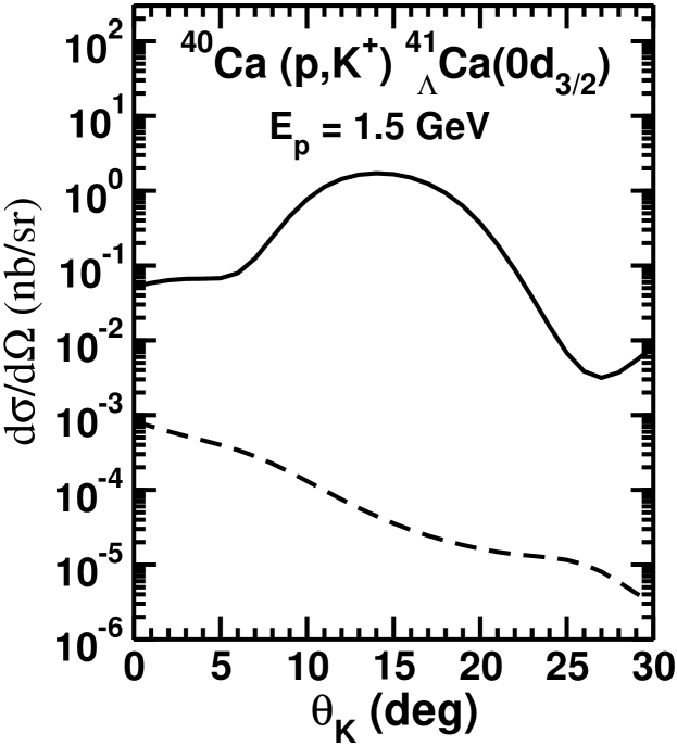
Figure 7: Relative contributions of target emission (TE) (solid line) and projectile emission (PE) (dashed line) graphs to the differential cross section for the ⁴⁰Ca$(p,K^{+})$${}^{41}\!\!\!_{\Lambda}$Ca$(0d_{3/2})$ reaction at the beam energy of 1.5 GeV. Only pion-exchange graphs are included in these calculations. The pion self-energy used in these calculations has been renormalized by using the Landau parameter $g^{\prime}=0.5$.

In the PE graph the values of the time-like momentum component $q_{0}$ in the meson propagator is taken to be $q_{0}=E_{i}$, where the latter is the energy of the incident proton (ignoring the nucleon binding energies) by the energy conservation at the vertices. Due to this the meson propagator in this diagrams [Fig. 2(c)] may develop a pole in the integration at $|q|=\sqrt{|q|^{2}+m_{\lambda}^{2}}$ ($m_{\lambda}$ is the mass of the meson). With the inclusion of the self-energy (which, in general, is complex at non-zero energies), the pole is automatically removed from the real axis and the pole integration problem disappears and the graph 2(c) becomes well behaved. Furthermore, this leads to a strong reduction in the contributions of this graph.

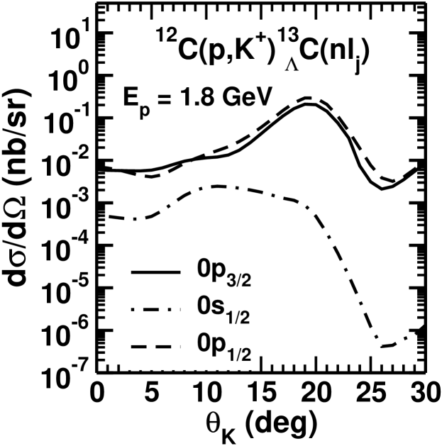
Figure 8: Differential cross section for the ¹²C$(p,K^{+})$${}^{13}\!\!\!_{\Lambda}$C reaction for the incident proton energy of 1.8 GeV for various bound states of final hypernucleus as indicated in the figure. The $\Lambda$ separation energies for various states were the same as those shown in Table 2.

On the other hand, such a pole does not develop in the TE diagram [Fig. 2(b)] since in this case the pion self-energy is real and attractive due to $q_{0}\approx 0$ [as can be seen from Fig. 3 of Ref. [25]]. This leads to a small denominator of the pion propagator leading to a consequent increase in the contribution of this graph. In fact this amplitude dominates the $(p,K^{+})$ cross sections as can be seen from Fig. 7 where we show the relative contributions of graph 2(b) and 2(c) to this cross section considering only the one pion exchange mechanism. Similar domination of the TE amplitudes have also been seen in case of the TNM calculations of the ($p,\pi$) reaction [19].

In Figs. 8 and 9, we show the kaon angular distributions corresponding to various final hypernuclear states excited in reactions ¹²C$(p,K^{+})$${}^{13}\!\!\!_{\Lambda}$C and
⁴⁰Ca$(p,K^{+})$${}^{41}\!\!\!_{\Lambda}$Ca, respectively. The incident proton energies in the two cases are taken to be 1.8 GeV and 1.5 GeV, respectively where the angle integrated cross sections for the two reactions are maximum. In both the cases we have taken the Landau parameter $g^{\prime}=0.5$ in the calculations of the pion self energy. The calculations are the coherent sum of all the amplitudes corresponding to the various meson exchange processes and intermediate resonant states. Clearly, the cross sections are quite selective about the excited hypernuclear state, being maximum for the state of largest orbital angular momentum. This is due to the large momentum transfer involved in this reaction. It may be noted that in each case the angular distribution has a maximum at angles larger than 0^∘. This is due to the fact that there are several maxima in the upper and lower components of the momentum space bound spinors in the region of large momentum transfers. Therefore, in the kaon angular distribution the first maximum may shift to larger angles reflecting the fact that the bound state wave functions show diffractive structure at higher momentum transfers.

We see that while in Fig. (8) there is a difference of more than an order of magnitude between the cross sections for the $p$-shell and the $s$-shell excitations, the two are almost of the same order of magnitude in Fig. 9. To understand this, we note from Table 2 that for the ${}^{13}\!\!\!_{\Lambda}$C hypernucleus, the binding energies of the $p$-shell states are in the range of only 0.70-0.90 MeV as compared to 11.69 MeV of the $s$-shell state. The bound state spinor ($\Phi$) behaves, at larger momentum transfers, approximately as $\frac{1}{k^{2}}$ where $k^{2}\propto\epsilon$. Thus, with increasing binding energies the magnitudes of $\Phi$ decreases at larger momenta. This leads to a decrease in the cross sections of those processes which are more sensitive to the larger momentum transfers. The $p$-shell state spinors in ${}^{13}\!\!\!_{\Lambda}$C, are considerably larger than those of the $s$ state in the relevant momentum transfer ($q$) region ($\sim$ 2-4 fm^-1). Therefore, the $p$-shell transitions are enhanced as compared to the $s$-shell one. Due to this binding energy selectivity, we call the reaction leading to the $p$-shell excitation as a matched transition while that to the $s$-shell a mismatched one.

On the other hand, both $p$- and $s$-shell transitions in Fig. 9 are strongly mismatched due to the fact that for the ${}^{41}\!\!\!_{\Lambda}$Ca hypernucleus both these states have large binding energies as compared to those of the $d$-shell. In this case, the spinors of the $p$- and $s$-states do not differ substantially from each other in the relevant $q$ region, which in turn makes the corresponding cross sections not to differ too much from each other. As a matter of fact, states with larger angular momenta are squeezed in the coordinate space (r-space) due to the centrifugal barrier and hence they are spread out in the momentum space (q-space) which enhances the cross sections for correponding transitions. It should, however, be mentioned here that for a fixed angular momentum, states with larger binding are more compact in r-space, and therefore are wider in q-space. Hence, in such cases cross sections to states with larger binding may actually be larger.

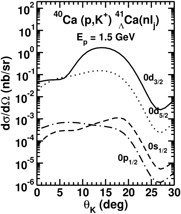
Figure 9: Differential cross section for the ⁴⁰Ca$(p,K^{+})$${}^{41}\!\!\!_{\Lambda}$Ca reaction for the incident proton energy of 1.5 GeV for various bound states of final hypernucleus as indicated in the figure. The $\Lambda$ separation energies for various states were as shown in Table 2.

The absolute magnitudes of the cross sections near the peak is around 1-2 nb/sr, although the distortion effects could reduce these values as is shown below. This order of magnitude estimates should be useful in planning of the future experiments for this reaction. As found in Ref. [25] contributions from the $N^{*}$(1710) resonance dominate the total cross section in each case. We also note that the interference terms of the amplitudes corresponding to various resonances are not negligible. It should be emphasized that we have no freedom in choosing the relative signs of the interference terms.

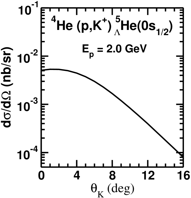
Figure 10: Differential cross section for the ⁴He$(p,K^{+})$${}^{5}\!\!\!_{\Lambda}$He reaction for the incident proton energy of 2.0 GeV for the bound state of final hypernucleus as indicated in the figure. The $\Lambda$ separation energy was as shown in Table 2.

In Fig. (10), we show the kaon angular distributions for reaction ⁴He$(p,K^{+})$${}^{5}\!\!\!_{\Lambda}$He leading to the $0s_{1/2}$ state of the hypernucleus at the proton beam energy of 2.0 GeV. In contrast to Figs 8 and 9, the maximum in the cross section, in this case, occurs at zero degree and it decreases gradually as the angle increases. This difference in the pattern of angular distribution seen in Fig. 10 from that of Figs. 8 and 9 can be understood from the fact that for momentum transfers relevant to this case the Dirac spinors are smoothly varying and are devoid of structures as can be seen in Fig. 4. In any case, from the purely kinematical arguments it is clear that the maximum in the cross section for a $\ell=0$ transition is expected normally to occur at smaller angles as compared that for a $\ell\neq 0$ one. The absolute magnitude of the cross section at the forward angles, in this case, is about 0.02 nb/sr. This value is somewhat smaller than the upper limit of the experimental center of mass cross section deduced for this reaction in a very preliminary study made in Ref. [8] at a similar beam energy [8].

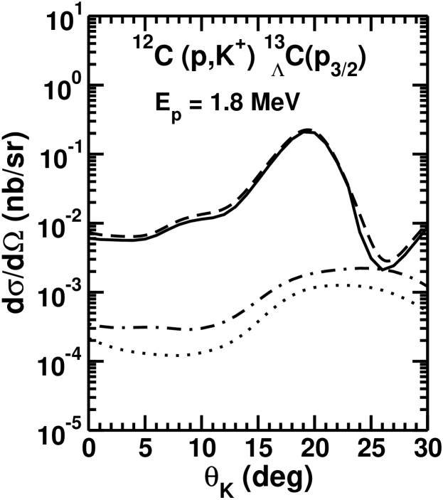
Figure 11: Differential cross section for the ¹²C$(p,K^{+})$${}^{13}\!\!\!_{\Lambda}$C$(0p_{3/2})$ reaction for the incident proton energy of 1.8 GeV. The dashed, dashed-dotted and dotted line show the contributions of $\pi$, $\rho$ and $\omega$ exchange processes, respectively. Their coherent sum is depicted by the full line.

In Fig. (11)-(12), we investigate the role of various meson exchange processes in describing the differential cross sections as a function of outgoing kaon angles for reactions ¹²C$(p,K^{+})$${}^{13}\!\!\!_{\Lambda}$C$(0p_{3/2})$, and ⁴⁰Ca$(p,K^{+})$${}^{41}\!\!\!_{\Lambda}$Ca$(0d_{3/2})$ at beam energies of 1.8 GeV, and 1.5 GeV, respectively. In each case, dashed, dashed-dotted and dotted lines show the contributions of $\pi$, $\rho$ and $\omega$ exchange processes, respectively. Their coherent sum is depicted by the full line. We note that pion exchange graphs dominate the production process for all angles in each case. This result is similar to the observation made in the case of associated kaon production in elementary $pp$ collisions [21, 56]. For the ¹²C$(p,K^{+})$${}^{13}\!\!\!_{\Lambda}$C$(0p_{3/2})$, and ⁴⁰Ca$(p,K^{+})$${}^{41}\!\!\!_{\Lambda}$Ca$(0d_{3/2})$ reactions, contributions of $\rho$ and $\omega$ exchange processes are unimportant at forward angles. However, at backward angles they become relatively more significant. This is understandable as at the backward angles the momentum transfer is larger which leads to greater contributions from the heavier meson exchanges. We see a destructive interference between the $\pi$ and $\rho$ contributions. The $\rho$ and $\omega$ exchange contributions put together do not affect appreciably the pion exchange only cross sections even at the backward angles due their mutual cancellation.

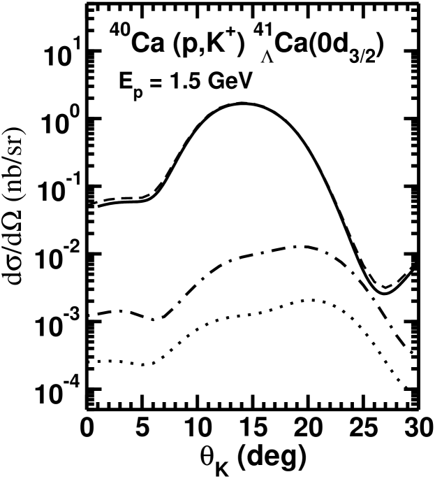
Figure 12: Differential cross section for the ⁴⁰Ca$(p,K^{+})$${}^{41}\!\!\!_{\Lambda}$Ca$(0d_{3/2})$ reaction for the incident proton energy of 1.5 GeV. various curves have the same meaning as in Fig. 11.

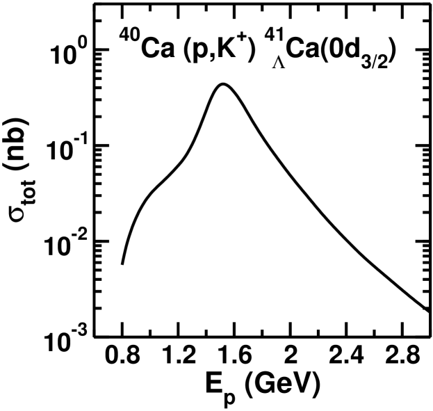
Figure 14: Angle integrated cross section for the ⁴⁰Ca$(p,K^{+})$${}^{41}\!\!\!_{\Lambda}$Ca$(0d_{3/2})$ reaction as a function of the incident proton beam energy.

In Figs. 13 and 14 we show the predicted beam energy dependence of the angle integrated cross sections for ¹²C$(p,K^{+})$${}^{13}\!\!\!_{\Lambda}$C$(0p_{3/2})$ and ⁴⁰Ca$(p,K^{+})$${}^{41}\!\!\!_{\Lambda}$Ca$(0d_{3/2})$ reactions, respectively. The results indicate a substantial dependence on the beam energy of the integrated cross sections. As the beam energy increases beyond the respective threshold energies, $E_{p}^{thres}$, the cross section first increases fast and then after peaking around a given value starts decreasing slowly. This trend is reminiscent of the general nature of the beam energy dependence of associate kaon production cross sections in elementary $pp$ collisions. The slight shift in the peak position towards the smaller value in the case of the heavier nucleus reflects the fact that the value of $E_{p}^{thres}$ is smaller as one goes to heavier target.

3.2.2 Effects of initial and final state interactions

Calculations presented thus far have been done in a plane wave approximation, where the proton-nucleus and kaon-nucleus interactions are ignored. While the essential features of the high momentum transfer reaction $(p,K^{+})$ can be understood in this approach, the nuclear interactions may have some consequences. They produce both absorptive and dispersive effects [57]. However, for large incident energies considered in this calculation, the absorption effects are likely to be the most important; a qualitative estimate of this is provided in the following.

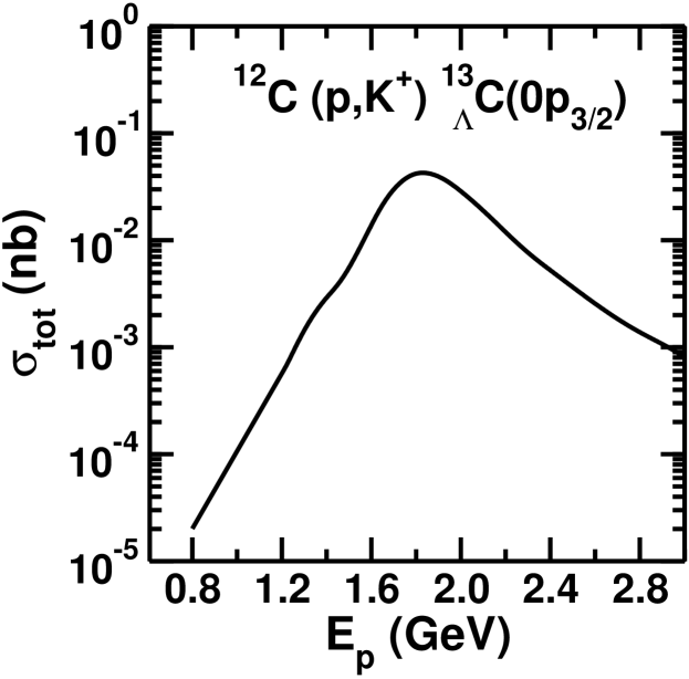
Figure 13: Angle integrated cross section for the ¹²C$(p,K^{+})$${}^{13}\!\!\!_{\Lambda}$C$(0p_{3/2})$ reaction as a function of the incident proton beam energy.

We use the eikonal approximation to estimate the attenuation factor for a particle traveling through the nuclear medium. First, we define a refractive index of the nuclear medium as (see, e.g., [58])

$$\eta(r,E) = \eta(E)\frac{\rho(r)}{\rho_{0}},$$ (39)

where $\rho(r)[\rho(\sqrt{b^{2}+z^{2}}]$ is the nuclear density distribution, and

$$\eta(E) = \frac{\kappa(E)}{k(E)}.$$ (40)

Here $k$ is the external wave number, and $\kappa$ is the wave number in the medium. The imaginary part of this refractive index is defined as $\eta_{0}$. In terms of $\eta_{0}$, the attenuation factor can be written as [45]

$$S(E) = \int\,d{\bf b}\,dz\,\frac{\rho({\bf b},z)exp[-k\,\eta_{0}(E)L(b)]}{\int\,d{\bf b}\,dz\,\rho({\bf b},z)},$$ (41)

where $L(b)$ is the length of the path traveled by the particle in the medium, which is given by

$$L(b) = \int_{0}^{\infty}\frac{\rho(r)}{\rho_{0}}\,dz$$ (42)

If the nuclear density is approximated by a Gaussian function,
$\rho(r)=\rho_{0}\,exp\,(-r^{2}/\alpha^{2})$, the integration in Eq. (41) can be done analytically. In this case the attenuation factor is given by

$$S(E) = \frac{1\,-\,exp[\,-\,\sqrt{\pi}\,\alpha\,k\,\eta_{0}(E)]}{\sqrt{\pi}\,k\,\eta_{0}(E)}$$ (43)

The attenuation due to medium can be calculated if the value of $\eta_{0}(E)$ is known. This can be obtained from the imaginary part of the optical potential $W_{0}$ as

$$\eta_{0}(E) = \frac{1}{\hbar^{2}}\frac{E}{k^{2}}W_{0}\,(E)$$ (44)

We use here the following high energy relations to obtain $W_{0}$

$$W_{0}\,(E) = \hbar^{2}\frac{k\,\sigma_{T}\rho_{0}}{2E},$$ (45)

where $\sigma_{T}$ is the total nucleon-nucleon or meson-nucleon cross section. In order to determine the total attenuation factor for the $(p,K^{+})$ reaction, the total attenuation due to both the proton and kaon distortions has been estimated by replacing the factor $k\eta_{0}$ in Eq. (43) by

$$k\eta_{0} \rightarrow k_{p}\eta_{0}(E_{p})+k_{K}\eta_{0}(E_{K})$$ (46)

In our estimation of the attenuation we have taken the average values of $\sigma_{T}$ as 45 mb and 14 mb for $pp$ [59] and $K^{+}p$ systems [60], respectively. The value of the parameter $\alpha$ is taken to be 1.61 fm, 2.37 fm and 3.52 fm for ⁴He, ¹²C and ⁴⁰Ca targets, respectively [61]. In Table 3, we show the values of the total attenuation $|S(E)|^{2}$ for the three targets discussed in this paper. We see that overall effect of initial and final state interactions is to decrease the peak cross sections relative to the PW calculations by a factor of 3 - 10. We however, would like to emphasize that these estimates only provide an idea of the absorptive effects. In more rigorous calculations, refractive distortion effects also play a role which could influence the shapes of the angular distributions as well.

Table 3: Total attenuation ($|S(E)|^{2}$) due to distortion effects in the initial and final channels.

Reaction	$|S(E)|^{2}$
4He$(p,K^{+})$${}^{5}\!\!\!_{\Lambda}$He$(0s_{1/2})$	0.28
12C$(p,K^{+})$${}^{13}\!\!\!_{\Lambda}$C$(0p_{3/2})$	0.19
40Ca$(p,K^{+})$${}^{41}\!\!\!_{\Lambda}$Ca$(0d_{3/2})$	0.10

At the same time, one should also note that in the distorted wave treatment the continuum wave functions are no longer associated with sharp momenta but are states with a momentum distribution [see Eqs (30)-(31)]. This leads to a redistribution of the large momentum transfer differently from what is allowed in the plane wave approximation. It could shift the sensitivity of the model to even lower momenta leading to enhanced cross sections. The competition between this effect and the absorption effect would ultimately decide the role of distortions in these reactions.

4 Summary and Conclusions

In summary, we have made a study of the $A(p,K^{+}){{}_{\Lambda}}B$ reaction on ⁴He, ¹²C, and ⁴⁰Ca targets within a fully covariant general two-nucleon mechanism where in the initial collision of the incident proton with one of the target nucleons, $N^{*}$(1710), $N^{*}$(1650), and $N^{*}$(1720) baryonic resonances are excited which subsequently propagate and decay into the relevant channel. The initial nucleon-nucleon collisions are mediated by pion and also by rho and omega exchange mechanisms. Expressions for the reaction amplitudes are derived in both distorted wave (DW) and plane wave (PW) approximations. However, the numerical calculations are performed within the latter approximation which helps in understanding the essential features of the $(p,K^{+})$ reaction without requiring very lengthy and cumbersome computations which are necessarily involved in the DW method. Wave functions of baryonic bound states are obtained by solving the Dirac equation with appropriate scalar and vector potentials.

In our model, the $(p,K^{+})$ reaction proceeds predominantly via excitation of the $N^{*}$(1710) resonant state. For reactions on all the three target nuclei, the cross sections are dominated by those graphs in which the intermediate meson originates from the target nucleon and the projectile nucleon gets excited to the baryonic resonance state (target emission graph). The one-pion-exchange processes make up most of the differential cross section at all angles. $\rho$ and $\omega$ exchange graphs individually are relatively more important at backward angles where the momentum transfer to the nucleus is comparatively larger. The effect of the heavier meson exchange is to reduce (although very weakly) the pion exchange only cross sections. However, the $\rho$ and $\omega$ exchange processes put together do not appreciably reduce the pion exchange only cross sections even at the back angles.

The calculated cross sections are maximum for the hypernuclear state with the largest orbital angular momentum. This is the typical of the large momentum transfer reactions [57]. For heavier targets, the angular distributions for the favored transitions peak at angles larger than the $0^{\circ}$ which in contrast to the results of most of the previous nonrelativistic calculations for this reaction. This reflects directly the nature of the Dirac spinors for the bound states which involve several maxima in the region of large momentum transfer. In case of the light target ⁴He, however, the differential cross section still peaks near the zero degree as in this case the momentum transfers are in the region where the bound state spinors are smoothly decreasing with momentum. The energy dependence of the calculated total production cross section follows closely that of the $pp\to p\Lambda K^{+}$ reaction.

The present results have been obtained using the PW approximation. Effects of initial and final state interactions have been estimated from an eikonal approximation for the nuclear elastic scattering interactions of the proton and kaon. The predicted cross sections are reduced by factors ranging between 3 - 10. The reduction is less for the lighter targets. However, In the present treatment we considered the absorptive distortions effects only which influence the absolute magnitudes of the cross sections. In a more rigorous calculation, distortions may also affect the shapes of the angular distributions.

Our results suggest that the study of the $(p,K^{+})$ reaction is attractive as it provides an alternative way to study the the spectroscopy of the $\Lambda$ hypernuclear states. This reaction should be measurable at the COSY facility in the Forschungszentrum Jülich. The characteristics of these cross sections predicted by us should be helpful in planning of such experiments. Such experiments may also lead to more quantitative calculations which should utilize the proper distorted waves.

5 ACKNOWLEDGMENTS

This work has been supported by the Forschungszentrum Jülich. We would like to thank Pascal Mühlich for helping us with the calculations of vector meson self-energies.

Appendix A Expression for the amplitudes in distorted wave and plane wave approximations

In this appendix we present the final form of the amplitude ($M_{2b}$) in both full distorted wave as well as plane wave approximations.

$$M_{2b}^{DW}(N^{*}_{1/2}) = -C_{iso}^{2b}\biggl{(}\frac{g_{NN\pi}}{2m_{N}}\biggr{)}(g_{N_{1/2}^{*}N\pi})(g_{N^{*}_{1/2}\Lambda K^{+}}){1\over{q^{2}-m_{\pi}^{2}-\Pi_{\pi}(q)}}$$ (47)

$$\times {1\over{p_{N^{*}}^{2}-(m_{N^{*}_{1/2}}-i\Gamma_{N^{*}_{1/2}}/2)^{2}}}\Biggl{[}{\mathscr{F}}_{1}(k_{1},k_{2})\sum_{m_{s}}Z_{\ell^{\prime}j}^{m_{j}m_{s}}({\hat{p}}_{1})Z_{\ell j}^{m_{j}m_{s}}({\hat{p}}_{2})^{*}$$

$$+ {\mathscr{F}}_{2}(k_{1},k_{2})\sum_{m_{s}}Z_{\ell j}^{m_{j}m_{s}}({\hat{p}}_{1})Z_{\ell^{\prime}j}^{m_{j}m_{s}}({\hat{p}}_{2})^{*}\Biggr{]}\sum_{L_{p}J_{p}\ell_{K}m_{K}}\sum_{\mu_{i}}(-)^{\ell_{K}}$$

$$\times <L_{p}01/2\mu_{i}|J_{p}\mu_{i}>\sqrt{2L_{p}+1}\,{\bf Y}_{\ell_{K}m_{K}}(\Omega_{K},\Omega_{K}^{\prime})$$

$$\times \Biggl{[}(c_{0}+c_{0}^{\prime}E_{K}){\mathscr{R}}_{\ell_{\Lambda}L_{p}\ell_{K}}Z_{L_{p}J_{P}}^{M_{p}\mu_{i}}({\hat{p}}^{\prime}_{i})Z_{\ell_{\Lambda}m_{j_{\Lambda}}-\mu_{i}}^{m_{j_{\Lambda}}\mu_{i}}({\hat{p}}_{\Lambda})^{*}$$

$$- ic_{0}^{\prime}{\mathscr{R}}_{\ell_{\Lambda}^{\prime}L_{p}\ell_{K}}\{(p_{K_{x}}^{\prime}-ip_{K_{y}}^{\prime})\sqrt{(1/2-\mu_{i})(3/2+\mu_{i})}$$

$$\times Z_{L_{p}J_{P}}^{M_{p}\mu_{i}}({\hat{p}}^{\prime}_{i})Z_{\ell_{\Lambda}^{\prime}m_{j_{\Lambda}}-\mu_{i}-1}^{m_{j_{\Lambda}}\mu_{i}+1}({\hat{p}}_{\Lambda})^{*}+(p_{K_{x}}^{\prime}+ip_{K_{y}}^{\prime})$$

$$\times \sqrt{(1/2+\mu_{i})(3/2-\mu_{i})}Z_{L_{p}J_{P}}^{M_{p}\mu_{i}}({\hat{p}}^{\prime}_{i})Z_{\ell_{\Lambda}^{\prime}m_{j_{\Lambda}}-\mu_{i}+1}^{m_{j_{\Lambda}}\mu_{i}-1}({\hat{p}}_{\Lambda})^{*}$$

$$+ 2p_{K_{z}}^{\prime}Z_{L_{p}J_{P}}^{M_{p}\mu_{i}}({\hat{p}}^{\prime}_{i})Z_{\ell_{\Lambda}^{\prime}m_{j_{\Lambda}}-\mu_{i}}^{m_{j_{\Lambda}}\mu_{i}}({\hat{p}}_{\Lambda})^{*}\}$$

$$- c_{0}^{\prime}{\mathscr{R}}_{\ell_{\Lambda}L_{p}^{\prime}\ell_{K}}\{(p_{K_{x}}^{\prime}-ip_{K_{y}}^{\prime})\sqrt{(1/2-\mu_{i})(3/2+\mu_{i})}$$

$$\times Z_{L_{p}^{\prime}J_{P}}^{M_{p}\mu_{i}}({\hat{p}}^{\prime}_{i})Z_{\ell_{\Lambda}m_{j_{\Lambda}}-\mu_{i}-1}^{m_{j_{\Lambda}}\mu_{i}+1}({\hat{p}}_{\Lambda})^{*}+(p_{K_{x}}^{\prime}+ip_{K_{y}}^{\prime})$$

$$\times \sqrt{(1/2+\mu_{i})(3/2-\mu_{i})}Z_{L_{p}^{\prime}J_{P}}^{M_{p}\mu_{i}}({\hat{p}}^{\prime}_{i})Z_{\ell_{\Lambda}m_{j_{\Lambda}}-\mu_{i}+1}^{m_{j_{\Lambda}}\mu_{i}-1}({\hat{p}}_{\Lambda})^{*}$$

$$+ 2p_{K_{z}}^{\prime}Z_{L_{p}^{\prime}J_{P}}^{M_{p}\mu_{i}}({\hat{p}}^{\prime}_{i})Z_{\ell_{\Lambda}m_{j_{\Lambda}}-\mu_{i}}^{m_{j_{\Lambda}}\mu_{i}}({\hat{p}}_{\Lambda})^{*}\}$$

$$+ i(-c_{0}+c_{0}^{\prime}E_{K}){\mathscr{R}}_{\ell_{\Lambda}^{\prime}L_{p}^{\prime}\ell_{K}}Z_{L_{p}^{\prime}J_{P}}^{M_{p}\mu_{i}}({\hat{p}}^{\prime}_{i})Z_{\ell_{\Lambda}^{\prime}m_{j_{\Lambda}}-\mu_{i}}^{m_{j_{\Lambda}}\mu_{i}}({\hat{p}}_{\Lambda})^{*}\Biggr{]},$$

where we have defined

$${\bf Y}_{\ell_{K}m_{K}}(\Omega_{K},\Omega_{K}^{\prime}) = Y_{\ell_{K}m_{K}}(\theta_{K},0)Y_{\ell_{K}m_{K}}^{*}(\theta_{K}^{\prime},\phi_{K}^{\prime}).$$ (48)

We have, $c_{0}=-m_{\Lambda}+m_{N^{*}}$, and $c_{0}^{\prime}=-1$. Superscript (*) on a function represents the complex conjugate of the function. In Eq. (A.1) we have defined

$$Z_{\ell j}^{m_{j}\mu}({\hat{p}}_{\lambda}) = <\ell m_{j}-\mu 1/2\mu|jm_{j}>Y_{\ell m_{j}-\mu}({\hat{p}}_{\lambda}),$$ (49)

$${\mathscr{F}}_{1}(k_{1},k_{2}) = 2Ag(k_{1})f(k_{2})+B\xi^{\prime}(k_{1})f(k_{2})+Bg(k_{1})\xi(k_{2}),$$ (50)

$${\mathscr{F}}_{2}(k_{1},k_{2}) = 2Af(k_{1})g(k_{2})+B\xi(k_{1})g(k_{2})+Bf(k_{1})\xi^{\prime}(k_{2}),$$ (51)

$${\mathscr{R}}_{\ell_{\Lambda}L_{p}\ell_{K}} = f_{\ell_{\Lambda}}(k_{\Lambda})F_{L_{p}J_{P}}(k^{\prime}_{i},k_{i})f_{\ell_{K}}(k_{K}^{\prime},k_{K}),$$ (52)

$${\mathscr{R}}_{\ell^{\prime}_{\Lambda}L_{p}\ell_{K}} = g_{\ell^{\prime}_{\Lambda}}(k_{\Lambda})F_{L_{p}J_{P}}(k^{\prime}_{i},k_{i})f_{\ell_{K}}(k_{K}^{\prime},k_{K}),$$ (53)

$${\mathscr{R}}_{\ell_{\Lambda}L_{p}^{\prime}\ell_{K}} = f_{\ell_{\Lambda}}(k_{\Lambda})G_{L_{p}^{\prime}J_{P}}(k^{\prime}_{i},k_{i})f_{\ell_{K}}(k_{K}^{\prime},k_{K}),$$ (54)

$${\mathscr{R}}_{\ell^{\prime}_{\Lambda}L_{p}^{\prime}\ell_{K}} = g_{\ell^{\prime}_{\Lambda}}(k_{\Lambda})G_{L_{p}^{\prime}J_{P}}(k^{\prime}_{i},k_{i})f_{\ell_{K}}(k_{K}^{\prime},k_{K}).$$ (55)

In Eqs. (A.4) and (A.5), $A=m_{N}$ and $B=1$. There is one more similar term in Eq. (A.1) involving wave function $\xi_{\ell}(k_{\Lambda})$ and $\xi_{\ell^{\prime}}^{\prime}(k_{\Lambda})$ in place of $f_{\ell}(k_{\Lambda})$ and $g_{\ell^{\prime}}(k_{\Lambda})$. In this term, coefficients $c_{0}$ and $c_{o}^{\prime}$ are replaced by $c_{1}$ and $c_{1}^{\prime}$ which are -1 and 0, respectively.

The form of the amplitude $M_{2b}$ in the plane wave approximation is

$$M_{2b}^{PW}(N^{*}_{1/2}) = -C_{iso}^{2b}\biggl{(}\frac{g_{NN\pi}}{2m_{N}}\biggr{)}(g_{N_{1/2}^{*}N\pi})(g_{N^{*}_{1/2}\Lambda K^{+}}){1\over{q^{2}-m_{\pi}^{2}-\Pi_{\pi}(q)}}$$ (56)

$$\times {1\over{p_{N^{*}}^{2}-(m_{N^{*}_{1/2}}-i\Gamma_{N^{*}_{1/2}}/2)^{2}}}\Biggl{[}{\mathscr{F}}_{1}(k_{1},k_{2})\sum_{m_{s}}Z_{\ell^{\prime}j}^{m_{j}m_{s}}({\hat{p}}_{1})Z_{\ell j}^{m_{j}m_{s}}({\hat{p}}_{2})^{*}$$

$$+ {\mathscr{F}}_{2}(k_{1},k_{2})\sum_{m_{s}}Z_{\ell j}^{m_{j}m_{s}}({\hat{p}}_{1})Z_{\ell^{\prime}j}^{m_{j}m_{s}}({\hat{p}}_{2})^{*}\Biggr{]}\Biggl{[}Z_{\ell_{\Lambda}j_{\Lambda}}^{m_{j_{\Lambda}}\mu_{i}}({\hat{p}}_{\Lambda})^{*}\,\,T_{1}$$

$$+ Z_{\ell_{\Lambda}^{\prime}j_{\Lambda}}^{m_{j_{\Lambda}}\mu_{i}}({\hat{p}}_{\Lambda})^{*}\,\mu_{i}\,\,T_{4}$$

$$+ Z_{\ell_{\Lambda}j_{\Lambda}}^{m_{j_{\Lambda}}\mu_{i}+1}({\hat{p}}_{\Lambda})^{*}\sqrt{(1/2-\mu_{i})(3/2+\mu_{i})}\,\,T_{2}$$

$$+ Z_{\ell_{\Lambda}j_{\Lambda}}^{m_{j_{\Lambda}}\mu_{i}-1}({\hat{p}}_{\Lambda})^{*}\sqrt{(1/2+\mu_{i})(3/2-\mu_{i})}\,\,T_{3}$$

$$+ Z_{\ell_{\Lambda}^{\prime}j_{\Lambda}}^{m_{j_{\Lambda}}\mu_{i}+1}({\hat{p}}_{\Lambda})^{*}\sqrt{(1/2-\mu_{i})(3/2+\mu_{i})}\,\,T_{5}$$

$$+ Z_{\ell_{\Lambda}^{\prime}j_{\Lambda}}^{m_{j_{\Lambda}}\mu_{i}-1}({\hat{p}}_{\Lambda})^{*}\sqrt{(1/2+\mu_{i})(3/2-\mu_{i})}\,\,T_{6}\Biggr{]},$$

where we have defined

$$T_{1} = (c_{0}+c_{0}^{\prime}\,E_{K})\,f(k_{\Lambda})-c_{0}^{\prime}{\frac{\hbar c}{E_{i}+m_{N}}}\,p_{i}p_{K}\,sin\,\theta_{K}\,f(k_{\Lambda})$$ (57)

$$+ (c_{1}+c_{1}^{\prime}\,E_{K})\,\xi(k_{\Lambda})c_{1}^{\prime}{\frac{\hbar c}{E_{i}+m_{N}}}\,p_{i}p_{K}\,cos\,\theta_{K}\,\xi(k_{\Lambda}),$$

$$T_{2} = c_{0}^{\prime}{\frac{\hbar c}{E_{i}+m_{N}}}\,p_{i}p_{K}\,sin\,\theta_{K}\,f(k_{\Lambda})$$ (58)

$$+ c_{1}^{\prime}{\frac{\hbar c}{E_{i}+m_{N}}}\,p_{i}p_{K}\,sin\,\theta_{K}\,\xi(k_{\Lambda}),$$

$$T_{3} = -T_{2},$$ (59)

$$T_{4} = -2i\,c_{0}^{\prime}\,p_{K}\,cos\,\theta_{K}\,g(k_{\Lambda})+2i\,{\frac{\hbar c}{E_{i}+m_{N}}}\,(-c_{0}+c_{0}^{\prime}\,E_{K})\,p_{i}\,g(k_{\Lambda})$$ (60)

$$- 2i\,c_{1}^{\prime}\,p_{K}\,cos\,\theta_{K}\,\xi^{\prime}(k_{\Lambda})+2i\,{\frac{\hbar c}{E_{i}+m_{N}}}\,(-c_{1}+c_{1}^{\prime}\,E_{K})\,p_{i}\,\xi^{\prime}(k_{\Lambda}),$$ (61)

$$T_{5} = -i\,c_{0}^{\prime}\,p_{K}\,sin\,\theta_{K}\,g(k_{\Lambda})--i\,c_{1}^{\prime}\,p_{K}\,sin\,\theta_{K}\,\xi^{\prime}(k_{\Lambda}),$$ (62)

$$T_{5} = T_{6}$$ (63)

The coefficients $c_{0}$, $c_{0}^{\prime}$, $c_{1}$ and $c_{1}^{\prime}$ are the same as defined above.

The amplitude for the graph 2(c) can be written in the analogous way. Those involving the excitation of other two resonances and vector meson exchanges have similar structure even though they may be a bit more complicated.

Appendix B Continuum distorted wave functions in momentum space

In this appendix we present a short derivation of Eqs. (30)-(31).

The incident and outgoing particles are described by stationary continuum wave functions $\Psi(r_{\alpha})=\psi_{\alpha}({\bf p}_{\alpha},{\bf r}_{\alpha})\,exp(-iE_{\alpha}t)$ where $\alpha$ = $i$ represents the incident channel and $K$ the outgoing one. $\psi_{\alpha}({\bf p}_{\alpha},{\bf r}_{\alpha})$ are given, in the partial wave representation, by

$$\psi_{i}^{(+)}({\bf p}_{i},{\bf r}_{i}) = \sum_{J_{p}L_{p}M_{p}}i^{L_{p}}<L_{p}M_{p}-\mu 1/2\mu|J_{p}M_{p}>Y^{*}_{L_{p}M_{p}-\mu}(\hat{p}_{i})$$ (64)

$$\times {{F^{C}_{L_{p}J_{p}}(k_{i},a_{i}){\mathscr{Y}}_{L_{p}1/2J_{p}}^{M_{p}}({\hat{r}}_{i})}\choose{G^{C}_{L^{\prime}_{p}J_{p}}(k_{i},a_{i}){\mathscr{Y}}_{L^{\prime}_{p}1/2J_{p}}^{M_{p}}({\hat{r}}_{i})}},$$

$$\phi_{K}^{(-)*}({\bf p}_{K},{\bf r}_{K}) = \sum_{\ell_{K}m_{K}}i^{-\ell_{K}}Y_{\ell_{K}m_{K}}({\hat{p}}_{K})f_{\ell_{K}}(k_{K},a_{K})Y_{\ell_{K}m_{K}}^{*}({\hat{r}}_{K}),$$ (65)

where various symbols have the same meaning as those described in the main text. Having chosen a momentum space formalism, we need to calculate the Fourier transforms

$$\Psi_{\alpha}(p^{\prime},p_{\alpha}) = \int\frac{d^{4}r_{\alpha}}{(2\pi)^{4}}e^{ip^{\prime}r_{\alpha}}\Psi_{\alpha}(r_{\alpha}),$$ (66)

depending on the unconstrained Fourier four momentum $p^{\prime}=(p^{\prime}_{0},{\bf p}^{\prime})$ and the asymptotic on-shell momenta $p_{\alpha}=(E_{\alpha},{\bf p}_{\alpha})$. The time integral in Eq. (B.3), can be trivially performed, leading to

$$\Psi_{\alpha}(p^{\prime},p_{\alpha}) = \delta(p^{\prime}_{0}-E_{\alpha})\int\frac{d^{3}{\bf r}_{\alpha}}{(2\pi)^{3}}e^{-i{\bf p}^{\prime}\cdot{\bf r_{\alpha}}}\psi_{\alpha}({\bf p}_{\alpha},{\bf r}_{\alpha}).$$ (67)

Further integrations in Eq. (B.4) can be carried out by using the relation

$$e^{-i{\bf p^{\prime}}\cdot{\bf r}_{\alpha}} = 4\pi\sum_{LM}i^{-L}j_{L}(k^{\prime}a_{\alpha})\,\,Y_{LM}({\hat{p}}^{\prime})\,\,Y_{LM}^{*}({\hat{r}}_{\alpha}),$$ (68)

which lead to Eqs. (30)-(31).

References

- [1] R. E. Chrien and C. B. Dover, Annu. Rev. Nucl. Part. Sci. 39 (1989) 113.
- [2] H. Bandō, T. Motoba and J. Žofka, Int. J. Mod. Phys. 5 (1990) 4021.
- [3] M. May et al., Phys. Rev. Lett. 47 (1981) 1106; E. H. Auerbach, A. J. Baltz, C. B. Dover, A. Gal, S. H. Kahana, L. Ludeking, and D. J. Milner, Phys. Rev. Lett. 47 (1981) 1110; M. May et al., Phys. Rev. Lett. 78 (1997) 4343; H. Kohri et al., Phys. Rev. C. 65 (2002) 034607.
- [4] C. Milner et al., Phys. Rev. Lett. 54 (1985) 1237; P. H. Pile et al., Phys. Rev. Lett. 66 (1991) 2585.
- [5] T. Hasegawa et al., Phys. Rev. C 53 (1996) 1210; H. Hotchi et al., Phys. Rev. Lett. 64 (2001) 044302.
- [6] E. Hiyama, M. Kamimura, T. Motoba, T. Yamada, and Y. Yamamoto, Phys. Rev. Lett. 85 (2000) 270; H. Nemura, Y. Akaishi, and Y. Suzuki, Phys. Rev. Lett. 89 (2002) 142504; F. Ineichen, D. Von-Eiff, and M.K. Weigel, J. Phys. G: Nucl. Part. Phys. 22 (1996) 1421; D. Vretenar, W. Poschl, G. A. Lalazissis, and P. Ring, Phys. Rev. C 57 (1998) 1060; P. Papazoglou, D. Zschiesche, S. Schramm, J. Schaffner-Bielich, H. Stöcker, and W. Greiner, Phys. Rev. C 59 (1999) 411; K. Tsushima, K. Saito, and A.W. Thomas, Phys. Lett. B 411 (1997) 9.
- [7] C. M. Keil, F. Hofmann, and H. Lenske, Phys. Rev. C 61 (2000) 064309; C. M. Keil and H. Lenske, Phys. Rev. C 66 (2002) 054307.
- [8] J. Kingler et al., Nucl. Phys. A634 (1998) 325.
- [9] O. B. W. Schult et al., Nucl. Phys. A585 (1995) 247c.
- [10] S. Shinmura, Y. Akaishi, and H. Tanaka, Prog. Theo. Physik 76 (1986) 157.
- [11] V. I. Komarov, A. V. Lado, and Yu. N. Uzikov, J. Phys. G: Nucl. Part. Phys. 21 (1995) L69.
- [12] V. N. Fetisov, Nucl. Phys. A639 (1998) 177c.
- [13] B. V. Krippa, Z. Phys. A 351 (1995) 411.
- [14] D. F. Fearing and G. Miller, Annu. Rev. Nucl. Part. Sci. 29 (1979) 121.
- [15] E. D. Cooper and H. S. Sherif, Phys. Rev. Lett. 47 818 (1982); Phys. Rev. C 25 (1982) 3024.
- [16] S. Frullani and J. Mougey, Adv. Nucl. Phys. 14 (1984) 1.
- [17] P. W. F. Alons, R. D. Bent, J. S. Conte, and M. Dillig, Nucl. Phys. A480 (1988) 413.
- [18] W. Peters, H. Lenske, and U. Mosel, Nucl. Phys. A640 (1998) 89; Nucl. Phys. A642 (1998) 506.
- [19] R. Shyam, W. Cassing and U. Mosel, Nucl. Phys. A586 (1995) 557.
- [20] M. V. Barnhill III, Nucl. Phys. A131 (1969) 106; L. D. Miller and H. J. Weber, Phys. Lett. 64B (1976) 279; R. Brockmann and M. Dillig, Phys. Rev. C 15 (1977) 361.
- [21] R. Shyam, Phys. Rev. C 60 (1999) 055213.
- [22] R. Shyam, G. Penner, and U. Mosel, Phys. Rev. C 63 (2001) 022202(R).
- [23] R. Shyam, Schriften des Forschungszentrum Jülich (series Matter and Materials) Vol. 21 (2004) 15.
- [24] R. Reuber, K. Hollinde, and J. Speth, Nucl. Phys. A570 (1994) 543.
- [25] R. Shyam, H. Lenske and U. Mosel, Phys. Rev. C 69 (2004) 065205.
- [26] N. Kaiser, Eur. Phys. J. A 5 (1999) 105.
- [27] A. Gasparian, J. Heidenbauer, C, Hanhart, L. Kodratyuk, and J. Speth, Phys. Lett. B 480 (2000) 273.
- [28] J. M. Laget, Phys. Lett. B 259 (1991) 24.
- [29] W. Schröder et al., Eur. Phys. J. A 18 (2003) 347.
- [30] M. Büscher, arXiv:nucl-exp/041010, Nucl. Phys. A754 (2005) 231c.
- [31] Göran Fäldt and Colin Wilkins, arXiv:nucl-th/0411019.
- [32] P. Moskal, M. Wolke, A. Khoukaz, and W. Oelert, Prog. Part. Nucl. Phys. 49 (2002) 1.
- [33] Landolt-Börnstein, New Series, edited by H. Schopper, I/12 (1988).
- [34] S. Sewerin et al., Phys. Rev. Lett. 83 (1999) 682; P. Kowina et al., arXiv:nucl-ex/0402008, Eur. Phys. J. A 22 (2004) 293.
- [35] J. D. Bjorken and S. D. Drell, Relativistic Quantum Mechaniscs, (McGraw-Hill, New York, 1964).
- [36] M. Benmerrouche, N.C. Mukhopadhyay, and J.F. Zhang, Phys. Rev.D 51 (1995) 3237.
- [37] M. Benmerrouche, R.M. Davidson and N.C. Mukhopadhyay, Phys. Rev.C 39 (1989) 2339.
- [38] T. Feuster and U. Mosel, Nucl. Phys.A 612 (1997) 375.
- [39] T. Feuster and U. Mosel, Phys. Rev.C 58, 457 (1998)
- [40] G. Penner and U. Mosel, Phys. Rev. C 66 (2002) 055211 (2002); 66 (2002) 055212.
- [41] V. Pascalutsa, Phys. Rev. D 58 (1998) 0960002; V. Pascalutsa and R. Timmermans, Phys. Rev. C 60 (1999) 042201(R); V. Pascalusta, Phys. Lett. B 503 (2001) 85.
- [42] R. Shyam and U. Mosel, Phys. Rev. C 67 (2003) 065202.
- [43] R. Shyam, A. Engel, W. Cassing, and U. Mosel, Phys. Lett. B273 (1991) 26.
- [44] V. F. Dmitriev and Toru Suzuki, Nucl. Phys. A438 (1985) 697.
- [45] B.K. Jain,J. T. Londergan, and G. E. Walker, Phys. Rev. C 37 (1988) 1564.
- [46] P. Mühlich, T. Falter and U. Mosel, Eur. Phys. J. A20 (2004) 499.
- [47] C. L. Korpa and M. F. M. Lutz, Nucl. Phys. A 742 (2004) 305.
- [48] S. Mallik, Eur. Phys. J. C 24 (2002) 143.
- [49] M. Effenberger, A. Hombach, S. Teis, and U. Mosel, Nucl. Phys. A613 (1997) 353.
- [50] H. Bethe and E.E. Saltpeter, Quantum mechanics of one and two electron atoms, springer, Berlin, 1957, p. 78.
- [51] A. S. Rosenthal and F. Tabakin, Phys. Rev. C 22 (1980) 711; S. R. Cotanch and F. Tabakin, Phys. Rev. C 15 (1977) 1379.
- [52] K. T. R. Davies, M. R. Strayer and G. D. White, J. Phys. G. 14 (1988) 961.
- [53] L. D. Miller and A. E. S. Green, Phys. Rev. C 5 (1972) 241.
- [54] R. Brockman, Phys. Rev. C 18 (1978) 1510.
- [55] B. D. Serot and J. D. Walecka, Adv. Nucl. Phys. 16 (1986) 1.
- [56] G. Fäldt and C. Wilkins, Z. Phys. A357 (1997) 241.
- [57] C. B. Dover, L. Ludeking and G. E. Walker, Phys. Rev.C 22 (1980) 2073.
- [58] T. E. O. Ericson and W. Weise, Pions and Nuclei, (Clarendon, Oxford, 1988).
- [59] D. V. Bugg, D. C. Salter, G. H. Stafford, R. F. George, K. F. Riley, and R. J. Tapper, Phys. Rev. C 146 (1966) 980.
- [60] P. K. Saha et al., Phys. Rev. C 70 (2004) 044613.
- [61] R. Hofstadter, Rev. Mod. Phys. 28 (1956) 214.