Abstract

The reaction $\gamma d\to\pi^{+}nn$ is calculated up to order $\chi^{5/2}$ in chiral perturbation theory, where $\chi$ denotes the ratio of the pion to the nucleon mass. Special emphasis is put on the role of nucleon–recoil corrections that are the source of contributions with fractional power in $\chi$. Using the known near threshold production amplitude for $\gamma p\to\pi^{+}n$ as the only input, the total cross section for $\gamma d\to\pi^{+}nn$ is described very well. A conservative estimate suggests that the theoretical uncertainty for the transition operator amounts to 3 % for the computed amplitude near threshold.

1 Introduction

Low–energy meson–nucleus reactions are of great interest for they are one of the best tools to deepen our understanding of the nuclear few–body problem. In particular, reaction involving the lightest member of the Goldstone octet, i.e. the pion, are subject of special experimental and theoretical efforts since they can be treated within chiral perturbation theory (ChPT). In this scheme high accuracy calculations in connection with reliable error estimates are possible. Indeed, since the pioneering works by Weinberg [1] and Gasser and Leutwyler [2] ChPT has developed into a powerful tool for investigations of the $\pi\pi$ [3], $\pi N$ [4] as well as few nucleon systems [5]. In addition, it was also Weinberg who pointed out how to calculate in an equally controlled way pion scattering off as well as inelastic reactions on nuclei [6]. There is also a large amount of work in the literature on neutral pion production (see Refs. [7, 8] and references therein) as well as on Compton scattering (see Refs. [9] and references therein) on the deuteron within ChPT.

In this paper we will present, for the first time, a complete calculation within ChPT up to order $\chi^{5/2}$ for the reaction $\gamma d\to\pi^{+}nn$, where the expansion parameter for the chiral expansion is denoted by $\chi=m_{\pi}/M_{N}$. Here $m_{\pi}$ ($M_{N}$) denotes the pion (nucleon) mass. Data on this channel exist for excess energies $Q=\sqrt{s}-(2M_{N}+m_{\pi})\leq 20$ MeV [10] which allow us to verify our results. The calculation is of high theoretical interest, because it provides an important test for our understanding of those aspects of $\pi NN$ dynamics that are relevant for pion production reactions on the deuteron. That understanding is a prerequisite for the reliable extraction of the pion photoproduction amplitude on the neutron, commonly done from corresponding deuteron data, but also for the determination of the $nn$ scattering length from $\pi^{+}$ production data.

In view of the high accuracy of the data and also because of the high reliability required for the extraction of the above mentioned quantities involving neutrons it is now time to critically investigate (and avoid whenever possible) the approximations traditionally used in pion reactions on few–nucleon systems. Here we will focus on approximations to the pion rescattering contribution as they are commonly used in both effective field theory calculations (see Ref. [11] and references therein) as well as phenomenological calculations (see Ref. [12] and references therein). Especially for the effective field theory calculations one might wonder how recoil corrections could be an issue, for the formalism allows for a rigorous expansion in $m_{\pi}/M_{N}$ that should build up the recoil corrections perturbatively. However, it was stressed recently [13] that the $\pi NN$ threshold introduces non–analyticities in the transition operators that call for special care: instead of being suppressed by one power in $m_{\pi}/M_{N}$ compared to the formally leading rescattering contributions (static term), as one might expect naively, the nucleon recoil terms turn out to scale as $\sqrt{m_{\pi}/M_{N}}$ relative to the static term as will be demonstrated in this paper. The only publication we are aware of, where the recoil corrections were treated properly for the near threshold region, is a phenomenological calculation for $\gamma d\to\pi^{0}d$ presented in Ref. [14] (so far most phenomenological studies concentrated on the $\Delta$–region, cf. Ref. [15] and references therein).

Recently the effect of the nucleon recoil on rescattering processes of pions in $\pi d$ scattering was studied [13, 16, 17] (for previous investigations on the role of the nucleon recoil see Refs. [18]). In particular, in Ref. [13] we demonstrated that, at least for the $\pi d$ system, the nucleon recoil can be neglected as long as the two–nucleon intermediate state is Pauli forbidden, while the pion is in flight. Thus, in this case the static approximation for the pion exchange is justified. However, as soon as the two–nucleon state is Pauli allowed, the nucleon recoil has to be included. In this case it turned out that the whole rescattering contribution (i.e. static term + recoil corrections) practically canceled completely. It should be stressed that for $\pi d$ elastic scattering the Pauli allowed two–nucleon intermediate states are anyhow suppressed by chiral symmetry.

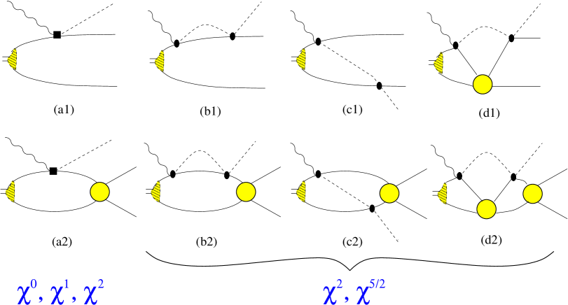
Figure 1: Diagrams for $\gamma d\to\pi^{+}nn$. Shown are one–body terms $\bigl{(}$diagram (a) and (b) $\bigr{)}$, as well as the corresponding rescattering contribution (c)—all without and with final state interaction. The need to include the $NN$ interaction non–perturbatively implies also the inclusion of diagrams with the two nucleon pair interacting, while a pion is in flight—this class is shown in diagrams (d). Solid straight, wiggly and dashed lines denote nucleons, photons and pions, in order. Filled squares and ellipses stand for the various vertices, the hatched area shows the deuteron wave function and the filled circle denotes the $nn$ scattering amplitude. Crossed terms (where the external lines are interchanged) are not shown explicitly. The tree level $\gamma p\to\pi^{+}n$ vertex, as it appears in diagram (a1) and (a2), contributes at leading order (order $\chi^{0}$), and order $\chi^{1}$ and $\chi^{2}$, depending on the one–body operator used. Loops start to contribute at order $\chi^{2}$, the corresponding recoil corrections enter at order $\chi^{5/2}$.

In this paper we will study the reaction $\gamma d\to\pi^{+}nn$ with special emphasis on the abovementioned recoil corrections. In this system the selection rules are such that the S-wave two–nucleon intermediate state during the pion rescattering process is allowed by the Pauli principle. In addition, once the strength of the one–body operator is fixed to the reaction $\gamma p\to\pi^{+}n$, no free parameters occur in the calculation for $\gamma d\to\pi^{+}nn$ to the order where the leading recoil corrections enter and thus we can compare our results to experimental data directly. At the same time we get a better understanding of the few–body corrections to $\gamma d\to\pi^{0}pn$. This reaction will eventually allow one to extract the amplitude of $\gamma n\to\pi^{0}n$ complementary to using $\gamma d\to\pi^{0}d$ discussed in Ref. [7]. Note that up to now no calculation for $\gamma d\to\pi^{+}nn$ exists where the nucleon recoil was properly included.

order	$s$–wave	$p$–wave	$d$–wave
$1$	$\chi_{m}^{0}$
$\chi^{1}$	$\chi_{m}^{1},\,\chi_{Q}^{2}$	$\chi_{Q}$
$\chi^{2}$	$\chi_{m}^{2},\,\chi_{Q}^{2}\chi_{m},\,\chi_{Q}^{4}$	$\chi_{Q}\chi_{m}$	$\chi_{Q}^{2}$
$\chi^{5/2}$	$\chi_{m}^{2}\chi_{Q},\,\chi_{m}^{5/2},\,\chi_{m}^{1/2}\chi_{Q}^{4}$

Table 1: Pattern of appearance of the expansion parameters $\chi_{m}=m_{\pi}/M_{N}$ and $\chi_{Q}=k_{\pi}/m_{\pi}$ on the amplitude level for a given order in $\chi$ for the total cross section. The first column shows the order parameter $\chi$, whereas the other three columns show the order assignments for the amplitudes of the various pion partial waves of relevance. Note, as we here consider the total cross section only, different partial waves do not interfere—this was used in the order assignment.

Before going into the details some comments are necessary regarding the relevant scales of the problem. In the near threshold regime of interest here (excess energies of at most 20 MeV above pion production threshold) the outgoing pion momenta are small compared even to the pion mass. Thus, in addition to the conventional expansion parameters of ChPT $m_{\pi}/\Lambda_{\chi}$ and $q_{\gamma}/\Lambda_{\chi}$, where $\Lambda_{\chi}$ denotes the chiral symmetry breaking scale of order of (and often identified with) the nucleon mass, and $q_{\gamma}$ denotes the photon momentum in the center–of–mass system which is of order of the pion mass, we can also regard $k_{\pi}/m_{\pi}$ as small, where $k_{\pi}$ denotes the outgoing pion momentum. In what follows we will perform an expansion in two parameters, namely

$$\chi_{m}=m_{\pi}/M_{N}\ \mbox{and}\ \chi_{Q}=k_{\pi}/m_{\pi}\ .$$

Obviously, the value of the second parameter depends on the excess energy. The energy regime of interest to us are excess energies up to 20 MeV. The maximum value of $\chi_{Q}$, $\chi_{Q}^{max}=\sqrt{2Q/m_{\pi}}$, possible at maximum energy is thus about 1/2. Since this is numerically close to $\sqrt{\chi_{m}}$ we use the following assignment for the expansion parameter

$$\chi\sim\chi_{m}\sim\chi_{Q}^{2}\ .$$ (1)

In this paper we will concentrate on total cross sections only and thus—up to one important exception—$\chi_{Q}$ appears with even powers only. In table 1 we show the powers of $\chi_{m}$ and $\chi_{Q}$ that appear in the amplitude as well as the corresponding order $\chi$ for the total cross section. The pertinent diagrams will be discussed in detail below. Note that the diagrams with $\pi N$ rescattering (see diagrams (b), (c) and (d) in Fig. 1) contribute at order $\chi_{m}^{2}$ as well as at $\chi_{m}^{2}\chi_{Q}$, $\chi_{m}^{5/2}$ and at $\chi_{m}^{1/2}\chi_{Q}^{4}$. The origin of the non–integer power of $\chi$ are the two–body ($\pi N$) and three–body $\pi NN$ singularities. This issue is discussed in detail in section 3.

The small pion momentum in the exit channel leads to a suppression of higher pion partial waves. As can be seen from table 1 we need to consider at most pion $d$–waves (here and in what follows we denote pion partial waves by small letters and $NN$ partial waves by capital letters). On the other hand, at excess energies of 20 MeV the maximum two nucleon momentum in units of the pion mass is of order 1 and thus there is a priori no suppression of higher $NN$ partial waves. However, since the $nn$ phase shifts are only sizable for $S$- and $P$-waves at the small energies of relevance, we only include the $nn$ final state interaction of those partial waves.

To summarize the scope of this work, it aims to improve the existing calculations for the reaction $\gamma d\to\pi^{+}nn$ in the following important aspects:

• A first complete ChPT calculation for the reaction $\gamma d\to\pi^{+}nn$ up to order $\chi^{5/2}$ is presented. At this order loops contribute and the non–perturbative character of the $NN$ interaction calls for the use of interacting two nucleon Green’s functions (leading to up to 3 loop diagrams as shown in diagram (d2) of Fig. 1).

• The leading nucleon recoil is included without approximation. It enters at order $\chi^{5/2}$.

• As always in effective field theory studies an estimation of the accuracy of the calculation can be given. A conservative estimate points at an accuracy of 2 % for the few–body corrections to the amplitude near threshold which is of the same order as the uncertainty of the input quantity $E_{0+}$—the invariant electric dipole amplitude for $\gamma p\to\pi^{+}n$ at threshold. Adding the two uncertainties in quadrature we arrive at a total uncertainty of 3 % for the full transition operator. In this work we use phenomenological $NN$ wavefunctions and thus we are not in the position to estimate the uncertainty of the complete matrix elements (see the corresponding discussion in the summary).

• For the first time pion $p$– and $d$–waves as well as the final state interaction in the $NN$ $P$–waves are included in a calculation for the near threshold regime. Note that the significance of $NN$ $P$–waves even at photon energies below 20 MeV was established long ago [19], however, so far they were only considered as plane waves in the impulse term (thus only through diagram (a1) of Fig. 1).

Our paper is structured as follows: in the next section we briefly review the central findings of Ref. [13]. The three–body dynamics is discussed in detail in section 3. The same formalism as described for $\pi d$ scattering in section 2 is applied to the reaction $\gamma d\to\pi^{+}nn$ in section 4. In section 5 we present the results followed by a brief summary. The details of the calculation for the various diagrams are given in appendices.

2 Remarks on the $\pi d$ system

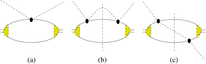
Figure 2: Typical diagrams for $\pi d$ scattering. Shown are one–body terms $\bigl{(}$diagram (a) and (b), as well as the corresponding rescattering contribution (c)$\bigr{)}$. Crossed terms (where the external pion lines are interchanged) are not shown explicitly.

To keep the paper self–contained, in this section we briefly review the findings of Ref. [13]. The relevant diagrams for $\pi d$ scattering are shown in Fig. 2. Diagram (a) denotes the tree level one–body contribution, diagram (b) the loop correction to the one–body piece and diagram (c) the rescattering term. It should be clear that the Pauli principle calls for a consistent simultaneous treatment of (b) and (c), for an interchange of the two nucleons while the pion is in flight (this intermediate state is marked by the perpendicular line in Fig. 2) transforms one diagram into the other.

The calculations of Ref. [13] were based on the effective $\pi N$ vertex,

$$V^{ba}_{\pi N}=\delta^{ba}g_{+}+\frac{i}{\sqrt{2}}\epsilon^{abc}\tau^{c}g_{-}\ ,$$ (2)

where $a,b,$ and $c$ are the Cartesian pion indices. We note that this vertex leads, up to corrections of $O(m_{\pi}/M_{N})$, to identical results for the $\pi d$ scattering length as the leading order chirally symmetric $\pi N$ interaction (the Weinberg–Tomozawa term) if we choose $g_{-}=-\sqrt{2}m_{\pi}/(2f_{\pi}^{2})$ and $g_{+}=0$. However, to keep the expressions simple we will use the notation of Ref. [13].

The main issue of Ref. [13] was to properly isolate the single nucleon contribution (the one that would be measured in $\pi N$ scattering) from the few body corrections. It is clear that part of diagram (b) contributes to the former and part to the latter. As outlined in Ref. [13] the proper prescription to separate these two pieces is to add to the tree level scattering (diagram (a)) the single nucleon one–loop contribution on the free nucleon at rest—this sum is the expression for the $\pi N$ scattering length, $a^{(1-body)}$. The same loop needs to be subtracted from the full contribution depicted in diagram (b). This procedure at the same time renders the expression for the loop finite. This difference is a true two–nucleon operator. To obtain more symmetric, easier to interpret results we subtracted from the rescattering piece the expression for the static exchange, i.e. the contribution from diagram (c) of Fig. 2 calculated in the static limit. In order to leave the final result unchanged, this contribution needs to be added as $a^{(st)}_{LO}$ (and $a^{(st)}_{NLO}$) to the expression for the $\pi d$ scattering length. Thus, the full result for the $\pi d$ scattering length reads

$$a=a^{(1-body)}+a^{(st)}_{LO}+a^{(rec)}+a^{(st)}_{NLO}\ ,$$ (3)

where the individual contributions for the static (st), the recoil (rec) and the NLO corrections to the static term are given by

$$a^{(st)}_{LO}{=}(g_{+}^{2}{-}g_{-}^{2})I_{0}\ ;\ \ a^{(rec)}{=}{g_{+}^{2}}I_{+}{+}{g_{-}^{2}}I_{-}\ ;\ \ a^{(st)}_{NLO}{\simeq}{-}\frac{m_{\pi}}{M_{N}}(g_{+}^{2}{-}g_{-}^{2})I_{0}\ .$$ (4)

The integrals denoted by $I_{0}$ and $I_{\pm}$, given explicitly in Ref. [13], are evaluated numerically using the deuteron wave functions from the Bonn potential [20]:

$$I_{+}=-0.88~{}I_{0}\ ,\ \qquad I_{-}=-0.19~{}I_{0}~{}.$$

These numbers clearly reflect the claim made above: for the $\pi d$ system the isovector $\pi N$ interaction, proportional to $g_{-}$, leads to a Pauli blocked intermediate state and numerically we find that the recoil corrections lead only to a 20% correction (Integral $I_{-}$ is numerically small, $I_{-}\ll I_{0}$.). When the NLO pieces mentioned above are added, the correction resulting from recoil and NLO terms together is only 4% and thus the static pion exchange is a good approximation for the total rescattering contribution. On the other hand, the isoscalar $\pi N$ interaction leads to a Pauli allowed intermediate state and in this case the recoil corrections cancel 90% of the static exchange ($I_{+}$ is large and negative, $(I_{0}+I_{+})\ll I_{0}$). The inclusion of the NLO piece in this case further reduces the total rescattering contribution down to 3 % of the static term. Therefore, in this case estimating the total rescattering contribution by the static exchange only is a very poor approximation.

3 The role of the $\pi NN$ cuts

Figure 3: Notation used in the discussion of the $\pi NN$ intermediate state. The ellipses labeled $O_{1}$ and $O_{2}$ denote the transition operators for the various possible reactions; e.g. for $\gamma d\to\pi^{+}nn$ the operators $O_{1}$ and $O_{2}$ refer to $\gamma d\to\pi^{+}nn$ and $\pi^{+}nn\to\pi^{+}nn$, respectively.

In this section we discuss the role of the three–nucleon cuts in more general terms. All arguments presented for the three–body dynamics apply to pion–nuclear reactions in general (as, e.g., $\pi d$ scattering), however, in this section we will use only the reaction $\gamma d\to\pi^{+}nn$ as illustrative example.

Typical diagrams that contain a $\pi NN$ intermediate state (cf., e.g., diagram (c2) of Fig. 1 and the corresponding Eq. (33) in appendix A), can be cast into the following form by a proper choice of variables (and dropping terms of higher order in $m_{\pi}/M_{N}$)

$$I_{\pi NN}(Q)=\int\frac{dK_{\pi}K_{\pi}^{2}\,dP_{R}P_{R}^{2}}{(2\pi)^{6}}\frac{f(K_{\pi}^{2},P_{R}^{2})}{Q-K_{\pi}^{2}/(2m_{\pi})-P_{R}^{2}/M_{N}+i0}\ ,$$ (5)

where $K_{\pi}$ denotes the pion momentum and $P_{R}$ denotes the relative momentum of the two nucleons while the pion is in flight (c.f. Fig. 3). Using the static approximation means to expand the denominator of the integral in Eq. (5) in powers of $m_{\pi}/M_{N}$ before evaluation of the integral. Thus, we get in the static approximation

$$I_{\pi NN}^{(static)}(Q)=\int\frac{dK_{\pi}K_{\pi}^{2}\,dP_{R}P_{R}^{2}}{(2\pi)^{6}}\frac{f(K_{\pi}^{2},P_{R}^{2})}{Q-K_{\pi}^{2}/(2m_{\pi})+i0}+O\left(\frac{m_{\pi}}{M_{N}}\right)\ .$$ (6)

We will demonstrate now analytically (and in section 5 numerically) that this procedure misses an important contribution to $I_{\pi NN}$.

Above the pion production threshold the denominator in Eq. (5) has a three–body singularity that leads to an imaginary part. This imaginary part of $I_{\pi NN}$ can be calculated by the replacement

$$(Q-K_{\pi}^{2}/(2m_{\pi})-P_{R}^{2}/M_{N}+i0)^{-1}\ \to\ -i\pi\delta(Q-K_{\pi}^{2}/(2m_{\pi})-P_{R}^{2}/M_{N})\ .$$

Thus we find

$$I_{\pi NN}^{(cut)}(Q)=-i\pi m_{\pi}\int\frac{dP_{R}P_{R}^{2}}{(2\pi)^{6}}f(2m_{\pi}(Q-P_{R}^{2}/M_{N}),P_{R}^{2})\sqrt{2m_{\pi}(Q-P_{R}^{2}/M_{N})}\ .$$ (7)

From this formula we see that the imaginary parts of the pion loops in diagram (b2) and (c2) of Fig. 1 are finite and lead to a strongly energy–dependent contribution. As long as the momentum–dependence of the function $f$ can be neglected, this part of the amplitude grows like $Q^{2}$, i.e. like the three–body phase space. These are the contributions at order $\chi_{m}^{1/2}\chi_{Q}^{4}$ given in table 1. Note that the corresponding amplitudes without final state interaction ((b1) and (c1) of Fig. 1) do not have a three–body cut but only a two–body singularity. Thus their imaginary parts scale as $\chi_{m}^{2}\chi_{Q}$.

On the other hand, the unitarity cut contribution of $I_{\pi NN}^{(static)}$ reads

$$I_{\pi NN}^{(cut,static)}(Q)=-i\pi m_{\pi}\sqrt{2m_{\pi}Q}\int\frac{dP_{R}P_{R}^{2}}{(2\pi)^{6}}f(2m_{\pi}Q,P_{R}^{2})\ .$$

The most remarkable difference between $I_{\pi NN}^{(cut)}$ and $I_{\pi NN}^{(cut,static)}$ is that in contrast to the former the latter scales as $\sqrt{Q}$, i.e. like the two body phase space for all diagrams (even for those with final state interaction) and therefore shows an energy dependence that is completely wrong—and at variance even with perturbative three–body unitarity.

For values of $P_{R}$ with $Q>P_{R}^{2}/M_{N}$ the integral $I_{\pi NN}^{(cut)}(Q)$ (cf. Eq. (7)) contributes to the imaginary part of $I_{\pi NN}(Q)$ (cf. Eq. (5)). To evaluate the contribution of the cut to the real part, the square root needs to be analytically continued to negative values of its argument through

$$\sqrt{2m_{\pi}(Q-P_{R}^{2}/M_{N})}\to i\sqrt{2m_{\pi}(P_{R}^{2}/M_{N}-Q)}\ .$$

To demonstrate explicitly the impact of this, let us consider the case $Q=0$. Then we get

$$I_{\pi NN}^{(cut)}(0)=\pi m_{\pi}\sqrt{\frac{2m_{\pi}}{M_{N}}}\int\frac{dP_{R}P_{R}^{2}}{(2\pi)^{6}}f(-2m_{\pi}P_{R}^{2}/M_{N},P_{R}^{2})P_{R}\ .$$ (8)

The corresponding expression for $I_{\pi NN}^{(cut,static)}(0)$ vanishes. On the other hand, the expression for the leading static approximation (cf. Eq. (6)) gives at threshold

$$I_{\pi NN}^{(static)}(0)=-2m_{\pi}\int\frac{dP_{R}P_{R}^{2}dK_{\pi}}{(2\pi)^{6}}f(K_{\pi}^{2},P_{R}^{2})\ .$$ (9)

The static approximation Eq. (9) only acquires corrections analytic in $(m_{\pi}/M_{N})$ and thus misses the contribution of Eq. (8). In fact, Eq. (8) corresponds to the threshold value of the mentioned non–analytic contribution from the three–body intermediate state that is dropped in the static approxi-mation—the extension to arbitrary values of $Q$ is straightforward. However, the contribution from $I_{\pi NN}^{(cut)}$ is significant as one can see from a naive dimensional analysis where all momenta—even those in the integral measure—are replaced by their typical values:

$$I_{\pi NN}^{(cut)}\sim-\sqrt{\frac{m_{\pi}}{M_{N}}}I_{\pi NN}^{(static)}\ ,$$ (10)

as claimed in the introduction. Therefore, in general the static approximation is to be avoided! As one can see, the contributions from the nucleon recoil through the three–body singularities to both the real and the imaginary part of the amplitude appear to be down by $\sqrt{\chi}$ compared to the leading loop contribution (the static piece). To be more explicit they contribute at orders $\chi_{m}^{5/2}$ and $\chi_{m}^{1/2}\chi_{Q}^{4}$ (cf. table 1). On the other hand, if we expand the propagator in Eq. (5) before the integration, we only get terms analytic in the pion mass (order $\chi$ corrections to the static piece) and miss the most prominent correction.

Now we are in the position to discuss in more detail the conjecture presented in Ref. [13] as well as in the previous section, namely that in general for all those diagrams, where the $S$-wave two–nucleon intermediate state that appears while the pion is in flight is forbidden by the Pauli principle, the various recoil corrections largely cancel, while in case of Pauli allowed S-wave intermediate states they add coherently. In the latter case the net effect of the rescattering diagrams was claimed to be small due to a destructive interference between the recoil corrections and the leading rescattering contribution (the static term—cf. Eq. (6)). We will now discuss the two cases in the light of the discussion above. The essential observation is that the recoil corrections are the analytic continuation of the imaginary parts related to on–shell $\pi NN$ intermediate states.

Pauli forbidden intermediate states: in this case the imaginary contributions stemming from the three-body unitarity cut in diagrams of the type of (b2) and those from the type of (c2) of Fig. 1 need to cancel exactly, for the corresponding $\pi NN$ state is forbidden. As a consequence, there will also be a cancellation for the analytic continuations (see Eq. (7)), i.e. for the corresponding principal value (PV) integrals, and thus the recoil corrections necessarily cancel to a large degree. Since this statement is based solely on the Pauli principle it must hold for all reactions.

Pauli allowed intermediate states: contrary to the first option in this case the corresponding unitarity cut parts of the diagrams (b2) and (c2) of Fig. 1 add coherently and, as above, the same is to be true for their analytic continuation. It is not possible to claim in general that the recoil contribution from the PV integrals completely cancels the whole static term. However, as illustrated by the estimate of Eq. (10), the recoil corrections tend to be of the order of magnitude of the static term and tend to interfere destructively with it. Here we refer to the discussion in section 5 and to Fig. 10.

As we discussed in the previous section, the leading operator for $\pi N$ scattering acting on a deuteron leads to a $\pi NN$ state, where the $S$–wave is forbidden for the $NN$–pair by the Pauli principle. On the other hand, as will be outlined below, the leading operator for $\gamma N\to\pi N$, when acting on a deuteron field, leads to a $\pi NN$ state, where the $NN$–pair is allowed to be in an $S$–wave. Thus, in the reactions $\pi d\to\pi d$, $\pi d\to\gamma NN$, and $\gamma d\to\pi^{0}d$ the static approximation indeed accounts for a significant fraction of the few–body corrections, whereas in $\gamma d\to\pi^{+}nn$ and $\gamma d\to\gamma d$, when evaluated near the pion threshold, the static approximation is expected to work quite poorly. References for the corresponding calculations are given in the introduction.

4 The reaction $\gamma d\to\pi^{+}nn$

Figure 4: Diagrams that contribute to the one–body production operator in diagrams (a1) and (a2) of Fig. 1. Only tree level diagrams that contribute to $\gamma p\to\pi^{+}n$ up to order $\chi^{2}$ are shown. The dots denote loops that contibute to the $s$–wave amplitude at oder $\chi^{2}$ as those shown in Fig. 5 (b) and (c).

We will start with a discussion of the one–body contributions to be used in the diagrams of type (a1) and (a2) of Fig. 1.

At threshold the $\pi\gamma NN$ vertex at leading order ($\chi_{m}^{0}$) and at next–to–leading order ($\chi_{m}^{1}$) is given by the so–called Kroll–Ruderman (KR) term [21] and its recoil correction ,

$$\hat{V}_{\pi\gamma NN}^{KR}=ieg_{\pi N}\left(1-\frac{\omega_{\pi}}{2M_{N}}\right)\left(\vec{\epsilon}_{\gamma}\cdot\vec{\sigma}\right)\epsilon^{3ab}\tau^{b}\ ,$$ (11)

where $\vec{\epsilon}_{\gamma}$ denotes the photon polarization and $\omega_{\pi}$ is the energy of the outgoing pion. The corresponding diagram is shown as diagram (a) in Fig. 4. Note that we use $g_{\pi N}=13.4$ in the calculation and the charge $e$ is normalized such that the fine structure constant is given as $e^{2}/(4\pi)=\alpha=1/137.$ This vertex contributes to the one–nucleon operator (impulse term) as shown in diagram (a1) and (a2) of Fig. 1 and also provides the production vertex for the virtual pion to be rescattered. As the $\pi\gamma NN$ vertex is both spin and isospin dependent, now, in contrast to $\pi d$ scattering, for the rescattering contributions the two–nucleon intermediate state that occurs while the pion is in flight is allowed by the Pauli principle to be in an $S$–wave.

According to table 1 at order $\chi$ we also need to consider the leading correction in $\chi_{Q}^{2}$ to the $s$–wave as well as the leading $p$–wave contribution which is of order of $\chi_{Q}$. Both are provided by the diagram where the photon couples to the pion in flight corresponding to diagram (b) of Fig. 4.The corresponding expression for the effective $\pi\gamma NN$ vertex reads

$$\hat{V}_{\pi\gamma NN}^{(b)}={-ieg_{\pi N}}\vec{\sigma}\cdot\left(\vec{k}_{\pi}-\vec{q}_{\gamma}\right)\frac{\vec{\epsilon}_{\gamma}\cdot\vec{k}_{\pi}}{\omega_{\pi}|\vec{q}_{\gamma}\,|-\vec{k}_{\pi}\cdot\vec{q}_{\gamma}}\epsilon^{3ab}\tau^{b}\ ,$$ (12)

where $\omega_{\pi}$ denotes the energy of the outgoing pion. This vertex contributes to the leading p–waves (order $\chi_{Q}$ for the amplitude — order $\chi_{Q}^{2}=\chi$ for the total cross section), the leading energy dependence of the $s$–wave (order $\chi_{Q}^{2}$ for the amplitude as well as the cross section, for this term can interfere with the contribution of order $\chi^{0}$), as well as the leading $d$–waves (order $\chi_{Q}^{2}$ for the amplitude and thus order $\chi_{Q}^{4}=\chi^{2}$ for the cross section).

Figure 5: Typical pion loops that contribute to $\gamma p\to\pi^{+}n$. Crossed terms for diagrams (a) and (b) are not shown explicitly.

At order $\chi_{m}^{2}$ pion loops start to contribute to the $s$–wave part of the $\gamma p\to\pi^{+}n$ amplitude (see Fig. 5) and thus to the reaction $\gamma d\to\pi^{+}nn$ as well. The only additional vertex needed for the evaluation of these loops is given in Eq. (2) with $g_{-}=-\sqrt{2}m_{\pi}/(2f_{\pi}^{2})$ and $g_{+}=0$. The imaginary part of diagram (a) in Fig. 5 contributes at $\chi_{m}^{2}\chi_{Q}$ whereas the imaginary part of diagram (b) starts to contribute only at higher order ($\chi_{m}^{2}\chi_{Q}^{3}$) and is thus not explicitly included in the calculation. In contrast to the imaginary parts the real parts of some of those pion loops on a single nucleon are divergent and need to be regularized (e.g. diagram (c) of Fig. 5) . In the calculation of the reaction $\gamma d\to\pi^{+}nn$ we use a prescription similar to that used for $\pi d$ scattering, as described in the previous section. In practice this means to replace the expression of Eq. (11) by

$$\hat{V}_{eff}=i\kappa E_{0+}(\vec{\epsilon}_{\gamma}\cdot\vec{\sigma})\epsilon^{3ab}\tau^{b}\ ,$$ (13)

where $\kappa=4\pi\sqrt{2}\left(m_{\pi}+M_{N}\right)$. The experimental value of $E_{0+}$ from the reaction $\gamma p\to\pi^{+}n$ is [25]:

$$E_{0+}=(28.06\pm 0.27\pm 0.45)\times 10^{-3}m_{\pi}^{-1}.$$

This value coincides within errors with the result of ChPT up to order $\chi_{m}^{3}$ [26]:

$$E_{0+}=(28.2\pm 0.6)\times 10^{-3}m_{\pi}^{-1}.$$ (14)

Although this calculation was performed to higher order than what we aim at here, we will use the latter value as input quantity for the threshold value of $E_{0+}$ since the contribution of order $\chi_{m}^{3}$ are of the order of the assigned uncertainty.

It is straightforward to show that the $s$–wave contribution derived from Eq. (12) has the same operator structure as Eq. (13) and we may simply include its effect by replacing $E_{0+}$ in Eq. (13) by $E_{0+}(k_{\pi}^{2})$ defined up to order $\chi_{Q}^{4}$ through

$$E_{0+}(k_{\pi}^{2})=E_{0+}+E_{0+}^{\,\prime}\frac{k_{\pi}^{2}}{m_{\pi}^{2}}+E_{0+}^{\,\prime\prime}\frac{k_{\pi}^{4}}{m_{\pi}^{4}}\ .$$ (15)

The leading contribution to both coefficients $E_{0+}^{\,\prime}$ and $E_{0+}^{\,\prime\prime}$ can be calculated directly from Eq. (12). At next to leading order the energy dependence of the $\gamma\pi NN$ vertex enters as well (c.f. Eq. (11)). Especially, we find

$$E_{0+}^{\,\prime}=-\frac{eg_{\pi N}}{3\kappa}\left(1+\frac{m_{\pi}}{M_{N}}\right)=-11.3\times 10^{-3}m_{\pi}^{-1}\ ,$$

where $|\vec{q}_{\gamma}|=m_{\pi}(1-m_{\pi}/(8M_{N})+O(\chi^{2}))$ was evaluated in the center of mass system of the reaction $\gamma d\to\pi^{+}nn$ at threshold. The slope parameter $E_{0+}^{\,\prime}$ is calculated up to its leading and next–to–leading order. However, we anyhow assign an uncertainty of 10 % to this quantity, for higher order corrections are known to be enhanced by the $\Delta$ resonance [27]. The given value for $E_{0+}^{\,\prime}$ compares well to that from the dispersive analysis of the Mainz group [28] and is consistent with that used as input in Ref. [25] to extract $E_{0+}$ from the data.

At order $\chi^{2}$ for our reaction, additional diagrams contribute to the transition $\gamma p\to\pi^{+}n$ where the photon gets absorbed on the nucleon, e.g. through the magnetic moment, followed by pion emission (diagrams (c) in Fig. 4). Thus, they are accompanied by a one–nucleon intermediate state. These diagrams, when used as the one–body operator in diagram (a2) of Fig. 1, acquire a two–nucleon cut that leads to an imaginary amplitude even at threshold due to the kinematically allowed transition $\gamma d\to pn$ followed by $pn\to\pi^{+}nn$. However, this two–nucleon cut introduces a new (large) momentum scale $p\simeq\sqrt{m_{\pi}M_{N}}$ into the problem that calls for special care. According to the counting rules for pion production in $NN$ collisions [29], the contribution of this two–nucleon cut is therefore suppressed by $\chi_{m}^{3/2}$ compared to the rescattering diagram (c2) of Fig. 1. It is therefore justified within the ordering scheme used to replace the two–nucleon propagator by its static limit. The resulting contribution from the magnetic couplings to the $s$–wave pion production on the nucleon is already included in the effective operator of Eq. (13). For the pion $p$–waves we get the following expression for the sum of the $s$– and $u$–channel contributions of Fig. 4(c)

$$\hat{V}_{\pi\gamma NN}^{(c)}=-\frac{ieg_{\pi N}}{\sqrt{2}M_{n}m_{\pi}}\left(A+\vec{\sigma}\cdot\vec{B}\right)\ ,$$ (16)

where

$$A = i(\mu_{p}-\mu_{n})\vec{k}_{\pi}\cdot(\vec{\epsilon}_{\gamma}\times\vec{q}_{\gamma})\ ,$$ (17)

$$\vec{B} = -2\left(\vec{\epsilon}_{\gamma}\cdot\vec{p}\right)\vec{k}_{\pi}+(\mu_{p}+\mu_{n})\left((\vec{\epsilon}_{\gamma}\cdot\vec{k}_{\pi})\vec{q}_{\gamma}-(\vec{q}_{\gamma}\cdot\vec{k}_{\pi})\vec{\epsilon}_{\gamma}\right)\ .$$ (18)

Here $\vec{p}$ denotes the momentum of the incoming nucleon and $\mu_{p}=2.79$ and $\mu_{n}=-1.91$ denote the magnetic moments of the proton and the neutron, respectively. The operator $\hat{V}_{\pi\gamma NN}^{(c)}$ given by Eq. (16) was evaluated directly for the channel $\gamma p\to\pi^{+}n$. As a consequence the expression does not show any explicit isospin dependence and an isospin factor of $\sqrt{2}$ appears.

In Ref. [27] it is shown that the pion $p$–waves converge quite slowly: the next–to–leading order correction to the dominant $p$–wave multipoles $M_{1^{+}}$ and $M_{1^{-}}$ change the leading result by a factor of 2. The reason for this sizable correction is the large numerical value of $(\mu_{p}-\mu_{n})=4.7$. On the other hand, the contribution of the $A$–term to $\gamma d\to\pi^{+}nn$ is suppressed. One reason can be read off from Eq. (16) almost directly: since the $A$–term is a scalar in spin space, it will not change the total spin of the two nucleon system, when used as the one–body operator in diagram (a) of Fig. 1. Thus the final $nn$ state is in a spin–triplet state. However, in the near threshold regime of interest here, the simultaneous appearance of an $nn$ $P$–wave ($nn$ spin–triplet states are to have odd angular momenta as a consequence of the Pauli principle) and a pion $p$–wave is suppressed. In addition, it turns out that for the total cross section the $A$–term does not interfere with the leading pion $p$–wave contributions (the term proportional to $\vec{q}_{\gamma}$ in Eq. (12)) which leads to an additional suppression. For details on the latter point we refer to the explicit expressions given in appendix A. One should also note that like for the slope of the $s$–wave amplitude, the $\Delta$–isobar gives potentially large corrections to the $p$–wave amplitudes [27]. Thus we assign an uncertainty of 10% also to those.

At order $\chi^{2}$, pion rescattering diagrams (see diagrams (b), (c) and (d) in Fig. 1) start to contribute. Here the same diagrams contribute as previously discussed for $\pi d$ scattering, but with the first $\pi N$ interaction being replaced by the $\gamma N\to\pi N$ transition vertex. These diagrams are depicted in Fig. 1 (b2) and (c2). However, there is in addition a whole new class of diagrams, namely those without final state interaction (depicted as (b1) and (c1)). Another important difference to $\pi d$ scattering is that, as already mentioned above, the S-wave two–nucleon state—while the pion is in flight—is now allowed by the Pauli principle. This has two consequences: first of all we expect that the static approximation will not work for the rescattering contribution and, as a second consequence, now nothing prevents the two–nucleon system to interact while the pion is in flight. As the $NN$ interaction is to be taken into account to all orders, these diagrams are also potentially important. The latter statement becomes especially clear when observing that the scattering length in the $nn$ channel is quite large; note that in the limit of an infinite scattering length the diagrams (d1) and (d2) acquire a logarithmic infrared divergence. In fact, then the two–nucleon propagator behaves as if it would describe the propagation of a massless particle.

Starting from the vertices given by Eq. (11) and in the appendix of Ref. [22] it is straightforward to write down the corresponding matrix elements for the diagrams shown in Fig. 1. Note that all diagrams are evaluated in Coulomb gauge. This is a standard choice in ChPT calculations, for many diagrams with single photons are relegated to higher orders, such as those where the photon couples to the charge of the nucleon and of the deuteron, respectively.

Figure 6: Diagrams where the photon couples to the structure of the deuteron. These diagrams start to contribute only at order $\chi^{3}$ and are therefore not considered here.

Diagrams, where the photon couples to a rescattered pion in flight turn out to be strongly suppressed numerically compared to those shown in Fig. 1. The reason for this is twofold: their imaginary part is suppressed as a consequence of gauge invariance that forces the photon–pion coupling to be of the order of the (small) pion momentum in the loop and the appearance of a second pion propagator leads to an additional suppression. This is in complete analogy to $\pi d$ scattering as discussed in detail in Ref. [31]. In addition gauge invariance in principle also calls for the inclusion of diagrams, where the photon couples to the internal structure of the deuteron. Typical representatives of this class are shown in figure 6. However, it is easy to show that these diagrams are suppressed by at least one power of $\chi$ compared to the leading rescattering contribution and therefore start to contribute at most at order $\chi^{3}$ to $\gamma d\to\pi^{+}nn$. Therefore these diagrams are not included in the calculation. As a consequence, the diagrams given in Fig. 1 (together with Figs. 4 and 5) are all that contribute to the given order.

Details on how the various diagrams are evaluated are given in the appendix A. Especially, there it is explained how we dealt with the three–body singularities that occur in diagrams (c2), (b2), (d1), and (d2). We want to mention that we evaluated the loop diagrams for non–relativistic pions (see appendix A) for that largely simplified the numerics. We checked by direct evaluation of diagrams (c1) and (c2) for threshold kinematics that switching to relativistic pions changes the individual contributions to the amplitude by less than 4 %.

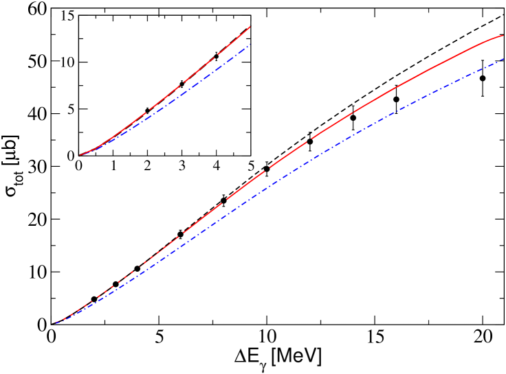
Figure 7: Total cross section of the reaction $\gamma d\to\pi^{+}nn$ at LO (dashed line), NLO (dash–dotted line) and $\chi^{5/2}$ order (solid line) together with experimental data from Ref. [10].

5 Results and discussion

In our calculations we use the standard values for the various constants, namely $f_{\pi}=92.4$ MeV, $m_{\pi}=139.57$ MeV (only the charged pions contribute to the order we are working) and $M_{N}=938.27$ MeV. The deuteron wave function and also the scattering wave functions needed for the $nn$ scattering amplitudes (in the ${}^{1}S_{0}$, ${}^{3}P_{0}$, ${}^{3}P_{1}$, and ${}^{3}P_{2}$ partial waves) are generated from the (charge–dependent) CD-Bonn potential [32]. Specifically, for the former we employ the analytical representation of the deuteron wave function provided in that reference because it allows us to perform some integrations analytically—see appendix B. For the same reason the scattering wave functions are computed from rank-1 separable representations of the CD-Bonn model, constructed along the lines of Ref. [33] utilizing the so-called Ernst–Shakin–Thaler method [34], cf. also appendix B. Note that the scattering length predicted by the CD-Bonn potential for the ${}^{1}S_{0}$ partial wave in the $nn$ system is $a_{nn}=-18.97$ fm [32], which is in line with most of the recent experimental information [35, 36] (note, the analysis of Ref. [37] gave a significantly lower value). We want to point out that in our calculation the contribution of the deuteron D-wave is included. This contribution to the leading diagrams is rather important, because it guarantees the correct normalization of the S-wave component for the potential used.

Although it would be desirable to use wave functions consistent with the transition operator, as provided, e.g., in Ref. [38], various studies show a low sensitivity to the wave function employed (see, e.g., [31]). In addition, the current operators have not yet been worked out to the same order and within the same unitary transformation as the $NN$ wave functions. We postpone this to a future study.

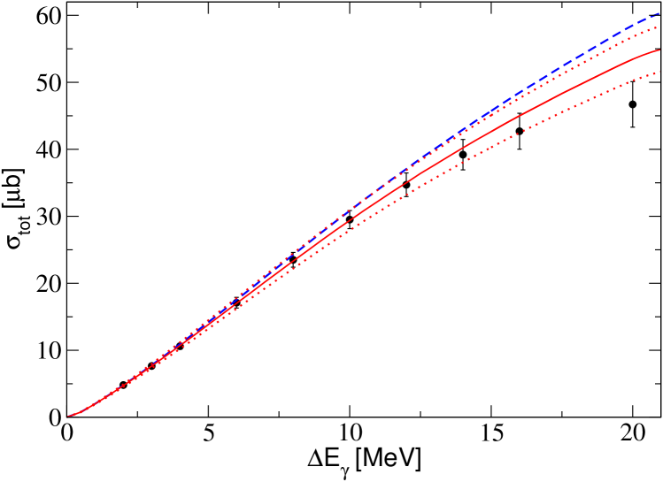
Figure 8: Importance of the slope parameter $E_{0+}^{\,\prime}$ defined in Eq. (15): The solid line shows the full result, whereas the long dashed line is produced with $E_{0+}^{\,\prime}=0$. The two dotted lines show the estimated uncertainty of full result as described in the text. The data are from Ref. [10].

The reaction $\gamma d\to\pi^{+}nn$ was calculated in the DWBA approximation by many authors in the middle of the seventies (cf., e.g., the review paper by Laget [19] and references therein). The approach used in those investigations corresponds to the evaluation of diagrams (a1) and (a2) of Fig. 1 using the $\gamma p\to\pi^{+}n$ vertex of Eq. (11); thus, in our language those were incomplete calculations up to next–to–leading order ($\chi$), because the energy dependence of the $\gamma\pi NN$ vertex and higher pion partial waves were neglected. Since the most important contribution to the $\gamma p\to\pi^{+}n$ operator in the near threshold region originates from the Kroll-Rudermann operator and its first correction (see Eq. (11)), which is known, and the convergence of diagram (a2) of Fig. 1 is provided by the universal fall-off of the deuteron wave function for small momenta (fixed by the deuteron binding energy) all those calculations led to very similar results (that we reproduce). To improve the calculations, some authors used instead of the prefactors of Eq. (11) the experimental input for $E_{0+}(k_{\pi}^{2})$ at threshold as the strength parameter for the one–body term (see, e.g., Ref. [10]). This, however, corresponds to an incomplete order-$\chi^{2}$ calculation, as discussed above. In addition, none of the works reported in Ref. [19] considered the $D$–wave of the deuteron consistently. The slope of $E_{0+}(k_{\pi}^{2})$, pion $p$–waves, or the $NN$ final state interaction in the $P$–waves were also not considered. The only attempt to improve the mentioned calculations via inclusion of a pion rescattering contribution was made in Ref. [39], where diagram (c2) of Fig. 1 was evaluated in the static limit, i.e. without nucleon recoil. This contribution was found to be large, amounting to an increase of around 10% of the total cross section (see the discussion of this question in Ref. [19]). However, as we stressed above, the static approximation is expected to work very poorly in this reaction.

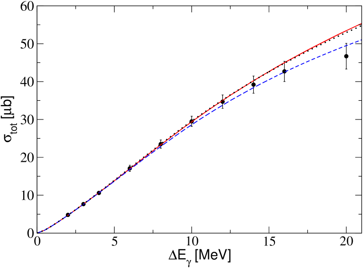
Figure 9: The role of the higher pion partial waves and effect of the $NN$ interaction in the $P$–wave. The dashed line shows the calculation where only the S-wave interactions are taken into account, the dotted line includes also the higher pion partial waves and the solid line includes in addition the contribution of the $NN$ final state interaction in the three possible included in diagram (a2) of Fig. 1.

Our results at order $\chi^{0}$, $\chi$ and combined order $\chi^{2}$ and $\chi^{5/2}$ are shown in Fig. 7 by the dashed, dash–dotted and solid lines, respectively. The data are taken from Ref. [10] and the energy is measured in terms of $\Delta E_{\gamma}=(1{+}m_{\pi}/(2M_{N}))Q$—the photon lab energy subtracted by its threshold value. Up to order $\chi^{1}$ the result is parameter free, i.e. it is determined by the value of $g_{\pi N}$ only. For the value of $E_{0+}(k_{\pi}^{2})$ at threshold that is needed as the only input quantity at order $\chi^{2}$, we use the central values of the ChPT calculation of Ref. [26] (that agrees with the experimental number, as mentioned in the previous section).

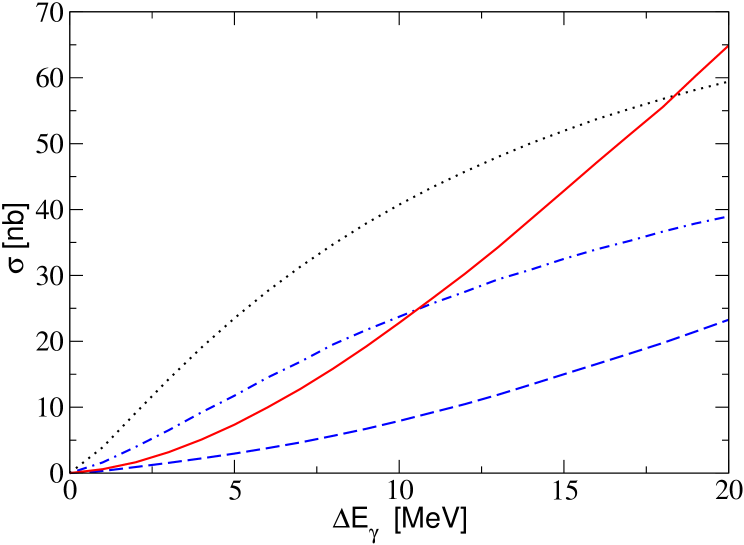
Figure 10: Quality of the static approximation for diagram (c2) of Fig. 1: The dash–dotted line shows the full calculation for diagram (c2), the dashed one that for diagram (b2), and the solid line the sum of the two. On the other hand, the result for diagram (c2) evaluated in the static approximation is given by the dotted line.

To illustrate the importance of the slope $E_{0+}^{\,\prime}$ we show in Fig. 8 both the full result as well as the one we get for a vanishing slope. For $\Delta E_{\gamma}$ larger than 10 MeV we observe a quite large sensitivity to the energy dependence of $E_{0+}(k_{\pi}^{2})$.

The counting scheme of Eq. (1) calls for an inclusion of $p$– and $d$–waves for the pion. The explicit expressions for the vertices are given in Eqs. (12) and (16). These vertices are to be considered embedded in diagrams (a1) and (a2) for Fig. 1 only. The contribution of the higher pion partial waves can be read off the difference of the dashed and the dotted line in Fig. 9.

The significance of $NN$ $P$–waves, even for $\Delta E_{\gamma}\leq 20$ MeV, was established long ago [19], however, so far they were only included as plane waves (through diagram (a1) of Fig. 1). In this work for the first time the final state interaction in the $NN$ $P$–waves is considered as well: we include the $NN$ interaction in the three possible $P$–waves (${}^{3}P_{0},^{3}P_{1}$ and ${}^{3}P_{2}$) in diagram $(a2)$. The effect of the nucleon $P$–waves on the total cross section is shown in Fig. 9. It is interesting to note that although the resulting effect of the $P$-wave $NN$ interaction is not significant for the total cross section the individual contributions of different partial waves are quite large (e.g., the ${}^{3}P_{1}$ partial wave enhances the cross section by about 15% at $\Delta E_{\gamma}=20$ MeV). It turns out that the contribution of the ${}^{3}P_{1}$ partial wave, which is enhanced due to constructive interference of the diagram (a1) and (a2) of Fig. 1 for this particular $NN$ partial wave, cancels to a large extent the contributions of the ${}^{3}P_{0}$ and ${}^{3}P_{2}$ partial waves. Note that the interference pattern of the various $NN$ $P$–waves can be traced to the fact that ${}^{3}P_{1}$ is repulsive, whereas ${}^{3}P_{0}$ and ${}^{3}P_{2}$ are attractive for small relative momenta. We have to mention that in the present calculation we neglect the coupling of the ${}^{3}P_{2}$ partial wave to the ${}^{3}F_{2}$. However, in view of the cancellation mentioned above this coupling might play a role, specifically because the mixing parameter $\epsilon_{2}$ is already about one third of the corresponding ${}^{3}P_{2}$ phase shift at $NN$ energies corresponding to $Q=20$ MeV. Also the $NN$ ${}^{1}D_{2}$ partial wave, which is likewise not included in the present calculation, should start to play a role with increasing energy. As mentioned above, the $NN$ wavefunctions used are not consistent with the transition operator. As long as this is not the case we do not think that including these probably minor effects is worth the effort. However, once wave functions consistent with the chiral counting are used, also the mentioned approximations need to be abandoned.

To summarize the results, we have calculated higher order chiral corrections to the impulse term used, e.g., in Ref. [19]. We found that due to a compensation amongst the effects of the various $NN$ $P$–waves, their net effect on the total cross section is negligible. In addition, the effect of the energy dependence of the pion $s$–wave production (parametrized by the slope $E_{0+}^{\prime}$) and of the pion $p$–waves compensated each other largerly as well. In view of this findings, the good agreement of the results of, e.g., Ref. [19] for the total cross section for photon energies above 10 MeV with the data should be considered accidental. However, for differential observables and especially for polarization observables we expect sizable effects from the chiral corrections calculated in this work.

Let us now discuss some of the results in detail. We found that all rescattering contributions of order $\chi^{2}$ and of order $\chi^{5/2}$ contribute with similar strength. This is true also for those diagrams where the $NN$ interaction appears inside the loop (diagrams (d1) and (d2) of Fig. 1). This clearly demonstrates the need to take into account the $NN$ $S$–wave interaction non–perturbatively also in intermediate states (as it is done routinely in three-nucleon calculations anyway).

Let us now compare in detail the results of different diagrams at the threshold. Here contributions from higher partial waves as well as those from the slope parameter $E_{0+}^{\prime}$ vanish. Therefore the uncertainty of the calculation in this regime can be estimated much more accurately than at higher energies. The results of the calculation of all possible contributions to the reaction amplitude at threshold are given in table 2. Evidently, the total contribution from few–body (rescattering) corrections to the full amplitude at threshold is about 5 % of the contribution from the distorted wave impulse approximation. One can also see from this table that the net contribution of the orders $\chi_{m}^{2}$ and $\chi_{m}^{5/2}$ cancels largely the NLO contribution (see also the corresponding results in Fig. 7 at low energies). Due to this one might speculate that corrections to this result from higher orders, especially from $\chi_{m}^{3}$, may influence the results stronger than suggested by the power counting. However we think that the uncertainty of the calculation at low energies is indeed within the uncertainty for $E_{0+}$ given by Eq. (14). Actually, no additional diagrams to those shown in Fig. 1 appear at order $\chi_{m}^{3}$. Thus, the contributions to the amplitude at this order originate basically from three sources:

1. NLO correction to the Kroll-Rudermann vertex when being used as a one–body operator in diagrams (b),(c) and (d) of Fig. 1 and the recoil corrections to the Weinberg–Tomozawa term. These corrections are of order $(m_{\pi}/2M_{N})\cdot 5\%=0.4\%$.

2. Relativistic corrections to the diagrams with pion rescattering. For diagram (c2) the relativistic correction gives only about 4% (to the 3 % contribution to the amplitude from diagram (c2)). Since there are no reasons a priori which could enhance the corresponding corrections to the other rescattering diagrams, we assign an uncertainty of order of 0.5 % to this effect.

3. The contributions from the coupling to the deuteron structure and the $nn$ scattering $T$–matrix. These are the hardest to estimate. However, as argued above, they are expected to be numerically quite small (see footnote # 6).

To summarize, we assign an uncertainty of 2 % to the few–body corrections of the amplitude. On the other hand the contribution at order $\chi_{m}^{3}$ to $E_{0+}$ at threshold is also about 2 % [26]. Adding these two uncertainties in quadrature we end up with a total uncertainty of 3 % for the transition operator near threshold. Unfortunately we are not in the position to estimate the uncertainty from the $NN$ interaction used—this has to be postponed until a calculation with fully consistent wave functions is performed.

In Fig. 8 the resulting uncertainty for the full calculation is shown by the two dotted lines. This range of uncertainties contains besides the 3 % just discussed also the 10 % uncertainties on both the pion $p$–waves as well as the slope parameter.

operator	order	diagrams	contribution
	$\chi_{m}^{0}$	(a1)+(a2)	1
one-body	$\chi_{m}^{1}$	(a1)+(a2)	$-$0.07
	$\chi_{m}^{2}$	(a1)+(a2)	$+$0.028
	$\chi_{m}^{5/2}$	(b2)	$-$0.016
	$\chi_{m}^{2}$,$\chi_{m}^{5/2}$	(c1)+(c2)	$+$0.039
few-body
	$\chi_{m}^{2}$,$\chi_{m}^{5/2}$	(d1)	$+$0.008
	$\chi_{m}^{2}$,$\chi_{m}^{5/2}$	(d2)	$+$0.024

Table 2: Contributions of different diagrams and operators to the reaction amplitude at threshold are given at different orders. The results in table are normalized to that of the calculation of diagrams (a1) + (a2) with the leading order Kroll-Rudermann vertex. Note that diagram (b1) does not contribute at threshold.

To show that the static exchange is indeed a poor approximation to the exact result for diagram (c2) of Fig. 1, as conjectured above, we compare in Fig. 10 the results for the static approximation with those from the exact calculation as well as with those for the one–body term (b2). As can be clearly seen, the static approximation fails to describe the full result in both strength as well as energy dependence. Evidently, for the exact calculation the total contribution of the sum of the results for (b2) and (c2) is extremely small near threshold, i.e. in the region where the real parts of both diagrams dominate. With increasing energy the contribution from the sum of these two diagrams increases rapidly. The reason for this effect is that at higher energies the role of the imaginary parts of both diagrams, which contribute coherently for the Pauli allowed $NN$ states, is growing rapidly. The resulting contribution for the sum of both diagrams of Figs. 2 (b2) and 2 (c2) to the total cross section does not exceed 4%.

6 Summary

In this paper we presented for the first time a ChPT calculation for the reaction $\gamma d\to\pi^{+}nn$. We calculated the diagrams displayed in Fig. 1—keeping explicitly the nucleon–recoil for the intermediate states. This corresponds to a complete calculation up to order $\chi^{5/2}$, where $\chi=m_{\pi}/M_{N}$.

The results of the full calculation are shown in Fig. 7 by the solid line. A good agreement between theory and experiment at low energies is obtained without any free parameter. The only input parameter was the threshold value for $E_{0+}$, taken from an N³LO calculation for $\gamma p\to\pi^{+}n$ [26]. Estimated conservatively, the uncertainty for the transition operator of our calculation is about 3 % in the amplitude for photon energies $\Delta E_{\gamma}$ below 5 MeV. Unfortunately we are not in the position to estimate the uncertainty from the $NN$ interaction used—this has to be postponed until a calculation with fully consistent wave functions is performed.

We found a strong suppression of the pionic rescattering contributions in comparison to the calculation in the frozen-nucleon approximation, i.e. in the static limit. This confirms the suggestion made in Ref. [19] and is in line with the general remark of our recent paper [13] where it was conjectured that the static limit is not adequate for pion rescattering processes with Pauli–allowed S-wave intermediate $NN$ states.

As a next step a fully consistent chiral perturbation theory calculation for the given reaction should be performed. It should include not only the use of wave functions constructed within this framework, as provided in Ref. [38], but also a re-evaluation of the transition operator within the same unitary transformation used to calculate the wave functions. Only then one can reliably asign a theoretical uncertainty to the full calculation and address questions raised in Ref. [42] for the consistency of the counting scheme and the scaling of four–nucleon operators. Although we do not expect the latter effects to be numerically significant for the reaction considered here, they are potentially important for $\gamma d\to\pi^{0}pn$, where the leading contribution vanishes.

Once a fully consistent ChPT calculation and better data are available for the reaction $\gamma d\to\pi^{+}nn$ one can consider to extract the energy dependence of $E_{0+}$ from this reaction, for the total cross section is very sensitive to the slope of $E_{0+}$, as illustrated in Fig. 8. However, before more definite conclusions can be drawn on this issue better data on the total cross section as well as the differential cross section in the energy regime of 15–25 MeV is needed.

The work presented allows one, amongst other things, to address the theoretical uncertainty of the $nn$ scattering length extracted from $\gamma d\to\pi^{+}nn$ analogously to the studies of Ref. [11] for $\pi^{-}d\to\gamma nn$. These studies are of high interest in the light of the significant differences in the values for $a_{nn}$ extracted from different groups in different reactions—c.f., e.g., Refs. [35, 36] and Ref. [37].

Acknowledgment

We are thankful to A.Gasparyan and L. Tiator for useful discussions. We also thank D.R. Phillips for a stimulating discussion and useful comments to the manuscript. This research is part of the EU Integrated Infrastructure Initiative Hadron Physics Project under contract number RII3-CT-2004-506078, and was supported also by the DFG-RFBR grant no. 02-02-04001 (436 RUS 113/652) and the DFG–Transregionaler–Sonderforschungsbereich SFB/TR 16 ”Subnuclear Structure of Matter”. A.E.K, and V.B. acknowledge the support of the Federal Programme of the Russian Ministry of Industry, Science, and Technology No 40.052.1.1.1112.

Figure 11: Definition of the various vectors of the problem.

Appendix A Matrix elements and observables

The differential cross section is related to the reaction amplitude via [40]

$$d\sigma=(2\pi)^{4}\delta^{(4)}(P_{f}-P_{i})\frac{1}{2}\frac{1}{4q_{\gamma}\sqrt{s}}|M_{fi}|^{2}\frac{d^{3}p_{1}}{(2\pi)^{3}2E_{1}}\frac{d^{3}p_{2}}{(2\pi)^{3}2E_{2}}\frac{d^{3}k_{\pi}}{(2\pi)^{3}2\omega_{\pi}},$$ (19)

where the indices 1 and 2 label momenta and energies of the final nucleons, and $k_{\pi}$ ($\omega_{\pi}$) denotes the pion three–momentum (energy), and $M_{fi}$ stands for the sum of all amplitudes given below: $M_{fi}=M_{a1}+M_{a2}+M_{b1}+\dots$  . The photon momentum is denoted by $q_{\gamma}$ and $\sqrt{s}=2M_{N}+m_{\pi}+Q$ where $M_{N}$ ($m_{\pi}$) and $Q$ are the nucleon (pion) mass and the excess energy, respectively. The choice of variables is illustrated in Fig. 11. The factor of 1/2 accounts for the two identical nucleons in the final state.

Let us now present the explicit expressions for the amplitudes corresponding to the diagrams in Fig. 1. All calculations are done in the center–of–mass system of the reaction. Note that in the calculation of the leading diagrams (a1) and (a2) in Fig. 1 the D-wave component of the deuteron wave function was taken into account, whereas in all other diagrams which are already suppressed by $\chi_{m}^{2}$ as compared to the leading ones, the inclusion of the D-wave is not necessary. This is also true for the diagrams with $NN$ $P$-wave final state interaction. The loops are evaluated using nonrelativistic kinematics even for the pion.

The calculation of the diagrams of Fig.1 were done using the standard Feynman rules with deuteron vertices (for details see, e.g., the appendix in Ref.[41] ). The explicit expressions for each individual term are:

1. Diagram a1.

$$M_{a1}=C_{NNLO}\ \chi_{1}^{\dagger}(\vec{\sigma}\vec{\epsilon}_{\gamma})\left[u(\vec{q}_{2})(\vec{\sigma}\vec{\epsilon}_{D}){-}\frac{w(\vec{q}_{2})}{\sqrt{2}}\left(3\frac{(\vec{\sigma}\vec{q}_{2})(\vec{q}_{2}\vec{\epsilon}_{D})}{q_{2}^{2}}-(\vec{\sigma}\vec{\epsilon}_{D})\right)\right]\frac{\sigma_{2}}{\sqrt{2}}\chi_{2}^{*}\ -(1\leftrightarrow 2)\ ,$$ (20)

where $C_{NNLO}=16\pi\sqrt{M_{N}}\left(M_{N}+m_{\pi}\right)E_{0+}$ , $\vec{q}_{1,2}=\vec{p}_{1,2}{+}\vec{q}_{\gamma}/2$, and $\vec{\epsilon}_{\gamma}$ and $\vec{\epsilon}_{D}$ are polarization vectors of the photon and the deuteron, respectively. The notation $-(1\leftrightarrow 2)$ points that one has to subtract the same term with spin and momentum variables of the two nucleons interchanged, in order to get properly anti–symmetrized amplitude.

Here $u(\vec{p})$ and $w(\vec{p})$ are the S-wave and D-wave deuteron wave functions defined in appendix B. The expression $\chi_{1}^{\dagger}\;\hat{O}\;\chi_{2}^{*}$ corresponds to the spin structure of the final $NN$ pair:

$$\chi_{1}^{\dagger}\;(\vec{\sigma}\vec{\epsilon}_{\gamma})(\vec{\sigma}\vec{\epsilon}_{D})\frac{\sigma_{2}}{\sqrt{2}}\;\chi_{2}^{*}=(\vec{\epsilon}_{\gamma}\vec{\epsilon}_{D})\left(\chi_{1}^{\dagger}\;\frac{\sigma_{2}}{\sqrt{2}}\;\chi_{2}^{*}\right){+}i(\vec{\epsilon}_{\gamma}\times\vec{\epsilon}_{D})\left(\chi_{1}^{\dagger}\;\vec{\sigma}\frac{\sigma_{2}}{\sqrt{2}}\;\chi_{2}^{*}\right)$$ (21)

and analogously for the D-wave part. Here the first and second terms on the r.h.s. are the spin-singlet and spin–triplet contributions, respectively ($\chi^{\dagger}\chi=1$).

2. Diagram (a2).

$$M_{a2}\!\!\! {=} \!\!\!-C_{NNLO}\ \frac{1}{2M_{N}}\int\frac{d^{3}p}{(2\pi)^{3}}\left\{\frac{{\cal M}^{0}_{NN}(\vec{p}{+}\vec{k}_{\pi}/2,\vec{p}_{12},E_{12})}{p_{12}^{2}\!-(\vec{p}{+}\vec{k}_{\pi}/2)^{2}\!+\!i0}u(\vec{p}{+}\vec{q}_{\gamma}/2)\ (\vec{\epsilon}_{\gamma}\vec{\epsilon}_{D})\left(\chi_{1}^{\dagger}\;\frac{\sigma_{2}}{\sqrt{2}}\;\chi_{2}^{*}\right)\right.$$ (22)

$$\qquad\qquad\qquad+\left.\frac{{\cal M}^{1}_{NN}(\vec{p}{+}\vec{k}_{\pi}/2,\vec{p}_{12},E_{12})_{\alpha\beta}}{p_{12}^{2}\!-(\vec{p}{+}\vec{k}_{\pi}/2)^{2}\!+\!i0}u(\vec{p}{+}\vec{q}_{\gamma}/2)\ i(\vec{\epsilon}_{\gamma}\times\vec{\epsilon}_{D})_{\beta}\left(\chi_{1}^{\dagger}\;\sigma_{\alpha}\frac{\sigma_{2}}{\sqrt{2}}\;\chi_{2}^{*}\right)\right\}\ ,$$

where $\vec{p}_{12}=(1/2)(\vec{p}_{1}-\vec{p}_{2})$ and the amplitudes ${\cal M}^{L}_{NN}$ are related to the $NN$ partial wave amplitudes with angular momentum $L$ as given below in this subsection. The energy of the $NN$ system is $E_{12}=p_{12}^{2}/M_{N}$ . The formula for $M_{a2}$ as given shows the contribution from the deuteron $S$–wave only. The inclusion of the $D$–wave in the convolution with ${}^{1}S_{0}$ $NN$ final state interaction is done like in the expression for diagram (a1). Note that this diagram is antisymmetrized as well, but in this case the antisymmetrization reduces just to an additional factor of two, so we have written the resulting expression explicitly. The same is done for all diagrams with the half off-shell $NN$ final state interaction, i.e. for the diagrams (b2), (c2), and (d2), and corresponding diagrams with pion higher partial waves.

The properly anti–symmetrized amplitude ${\cal M}_{NN}$ for the $S-$ and $P$-wave $NN$ interaction with isospin $1$ in the plane wave basis is

$$\langle\lambda_{1}^{\prime}\lambda_{2}^{\prime},\vec{p}\,^{\prime}|M(E)|\lambda_{1}\lambda_{2},\vec{p}\,\rangle\!\!\!\! = \!\!\!\!\!2\left(\chi_{\lambda_{1}^{\prime}}^{\dagger}\;\frac{\sigma_{2}}{\sqrt{2}}\;\chi_{\lambda_{2}^{\prime}}^{*}\right){\cal M}^{0}_{NN}(\vec{p},\vec{p}\,^{\prime},E)\left(\chi_{\lambda_{1}}^{T}\;\frac{\sigma_{2}}{\sqrt{2}}\;\chi_{\lambda_{2}}\right)$$ (23)

$$\qquad\quad+2\left(\chi_{\lambda_{1}^{\prime}}^{\dagger}\;\sigma_{\alpha}\frac{\sigma_{2}}{\sqrt{2}}\;\chi_{\lambda_{2}^{\prime}}^{*}\right){\cal M}^{1}_{NN}(\vec{p},\vec{p}\,^{\prime},E)_{\alpha\beta}\left(\chi_{\lambda_{2}}^{T}\;\frac{\sigma_{2}}{\sqrt{2}}\sigma_{\beta}\;\chi_{\lambda_{1}}\right)\ ,$$

where the first (second) term corresponds to the spin–singlet (spin–triplet) $NN$ states. Here $\lambda^{\prime}$ and $\lambda$ stand for the spin projections of final and initial nucleons, respectively, and $\chi_{\lambda}$ for corresponding spinors. The amplitudes ${\cal M}^{L}_{NN}$ in this formula are related to the standard $NN$ partial wave amplitudes $f^{JL}_{S}$, where $J$ denotes the total angular momentum, $L$ the angular momentum in the initial and final state (we do not consider couplings between partial waves with different angular momenta, e.g., the coupling of the ${}^{3}P_{2}$ to the ${}^{3}F_{2}$ partial wave), and $S$ the total spin, through

$${\cal M}^{0}_{NN}(\vec{p},\vec{p}\,^{\prime},E) = 16\pi M_{N}f^{00}_{0}(p^{\prime},p,E)$$

$${\cal M}^{1}_{NN}(\vec{p},\vec{p}\,^{\prime},E)_{\alpha\beta} = 16\pi M_{N}\sum_{J}(2J+1){\cal P}^{J}_{\alpha\beta}f^{J1}_{1}(p^{\prime},p,E)\ .$$ (24)

The $f^{JL}_{S}(p^{\prime},p,E)$ are related on the mass shell to the partial phase shifts via

$$f^{JL}_{S}(p,p,p^{2}/M_{N})=\frac{1}{2ip}\left(\exp(2i\delta^{JL}_{S})-1\right).$$

The projection operators for the various total angular momenta with $L=L^{\prime}=1$ and for the $S=1$ read

$${\cal P}^{0}_{\alpha\beta} = \hat{p}^{\prime}_{\alpha}\hat{p}_{\beta}\ ,$$

$${\cal P}^{1}_{\alpha\beta} = \frac{1}{2}\,\epsilon^{\alpha\lambda\tau}\epsilon^{\beta\rho\tau}\hat{p}^{\prime}_{\lambda}\hat{p}_{\rho}=\frac{1}{2}\left(\delta_{\alpha\beta}(\hat{p}\cdot\hat{p}^{\prime})-\hat{p}^{\prime}_{\beta}\hat{p}_{\alpha}\right)\ ,$$

$${\cal P}^{2}_{\alpha\beta} = \frac{3}{20}\left(\delta_{\lambda\alpha}\hat{p}_{\rho}^{\prime}+\delta_{\rho\alpha}\hat{p}_{\lambda}^{\prime}-\frac{2}{3}\delta_{\lambda\rho}\hat{p}_{\alpha}^{\prime}\right)\left(\delta_{\lambda\beta}\hat{p}_{\rho}+\delta_{\rho\beta}\hat{p}_{\lambda}-\frac{2}{3}\delta_{\lambda\rho}\hat{p}_{\beta}\right)$$

$$= \frac{3}{10}\left(\delta_{\alpha\beta}(\hat{p}\cdot\hat{p}^{\prime})+\hat{p}^{\prime}_{\beta}\hat{p}_{\alpha}-\frac{2}{3}\hat{p}^{\prime}_{\alpha}\hat{p}_{\beta}\right)\ ,$$

where $\hat{p}=\vec{p}/|\vec{p}\,|$ and analogously for $\hat{p}^{\prime}$. These projectors are normalized such that

$$\int d\Omega_{\vec{p}^{\prime}}{\cal P}^{J}_{\alpha\beta}{\cal P}^{J^{\prime}}_{\alpha\beta} = \frac{4\pi}{2J+1}\ \delta^{JJ^{\prime}},$$

and the total neutron-neutron cross-section reads then

$$\sigma^{nn}_{tot}=\frac{1}{2}\cdot 4\pi\sum_{JLS}\ (2J+1)|f^{JL}_{S}(p^{\prime},p,E)|^{2}\ .$$ (25)

Note that the factor of one half occurs in this expression because the nucleons are identical.

3. Diagram (b1).

The real part of the diagram (b1) renormalizes the bare vertex in the leading diagram (a1) resulting in the experimentally observed value $E_{0}^{+}$ for $\gamma p\to\pi^{+}n$ process. Thus, the real part of this diagram is already included in the expression for diagram (a1). The imaginary part of (b1) is

$$M_{b1}=iC_{LO}\frac{m_{\pi}}{8\pi(1+m_{\pi}/M_{N})f^{2}_{\pi}}\ u(\vec{p}_{2}\!{+}\!\vec{q}_{\gamma}/2)\ k_{\pi N_{1}}\chi_{1}^{\dagger}(\vec{\sigma}\vec{\epsilon}_{\gamma})(\vec{\sigma}\vec{\epsilon}_{D})\frac{\sigma_{2}}{\sqrt{2}}\chi_{2}^{*}-(1\leftrightarrow 2),$$ (26)

where $k_{\pi N_{i}}{=}|M_{N}\vec{k}_{\pi}{-}m_{\pi}\vec{p}_{i}|/(M_{N}{+}m_{\pi})$ is the magnitude of the relative momentum of the final pion and the final nucleon with momentum $p_{i}$ and $C_{LO}=4\sqrt{M_{N}}g_{\pi N}e/(\sqrt{2})$.

4. Diagram (c1).

$$M_{c1}=-C_{LO}\ \frac{m_{\pi}}{2(1+m_{\pi}/M_{N})f^{2}_{\pi}}\;I_{c_{1}}\;\chi_{1}^{\dagger}(\vec{\sigma}\vec{\epsilon}_{\gamma})(\vec{\sigma}\vec{\epsilon}_{D})\frac{\sigma_{2}}{\sqrt{2}}\chi_{2}^{*}\ -(1\leftrightarrow 2),$$ (27)

where the integral $I_{c_{1}}$ is

$$I_{c_{1}}=\int\frac{d^{3}p}{(2\pi)^{3}}\ \frac{u(\vec{p}\!+\!\vec{q}_{\gamma}/2)}{k_{\pi N_{1}}^{2}-(\vec{p}+\frac{M_{N}}{M_{N}+m_{\pi}}\vec{p}_{1})^{2}+i0}\ .$$ (28)

5. Diagram (b2)

$$M_{b_{2}}=C_{LO}\ \frac{1}{8M_{N}f_{\pi}^{2}}I_{b_{2}}(\vec{\epsilon}_{\gamma}\vec{\epsilon}_{D})\left(\chi_{1}^{\dagger}\;\frac{\sigma_{2}}{\sqrt{2}}\;\chi_{2}^{*}\right)\ ,$$ (29)

with

$$I_{b_{2}}=\int\frac{d^{3}pd^{3}l}{(2\pi)^{6}}\frac{{\cal M}^{0}_{NN}(\vec{p}{+}\vec{k}_{\pi}/2,\vec{p}_{12},E_{12})}{p^{2}_{12}{-}(\vec{p}{+}\vec{k}_{\pi}/2)^{2}{+}i0}\;\frac{u(\vec{p}{+}\vec{q}_{\gamma}/2)}{Q{-}\frac{p^{2}}{2M_{N}}{-}\frac{l^{2}}{2M_{N}}{-}\frac{(\vec{l}{+}\vec{p})^{2}}{2m_{\pi}}{+}i0}$$ (30)

The integral with the $\pi N$ loop, i.e. over $d^{3}l$, is divergent and has to be renormalized (cf. discussion of diagram (b1)). After renormalization it takes the form

$$I_{b_{2}}=\frac{-im_{\pi}}{2\pi(1{+}m_{\pi}/M_{N})}\int\frac{d^{3}p}{(2\pi)^{3}}\frac{{\cal M}^{0}_{NN}(\vec{p}{+}\vec{k}_{\pi}/2,\vec{p}_{12},E_{12})}{p^{2}_{12}{-}(\vec{p}{+}\vec{k}_{\pi}/2)^{2}{+}i0}\;u(\vec{p}{+}\vec{q}_{\gamma}/2)\;K(Q,p)\ ,$$ (31)

where $m_{\pi N}=m_{\pi}M_{N}/(M_{N}{+}m_{\pi})$, $\mu_{N}=M_{N}(M_{N}{+}m_{\pi})/(2M_{N}{+}m_{\pi})$, and

$$K(Q,p)=\sqrt{2m_{\pi N}(Q{-}p^{2}/2\mu_{N})}\ .$$

Note that for negative arguments the square root needs to be replaced by $i\sqrt{2m_{\pi N}(p^{2}/2\mu_{N}{-}Q)}$. Thus, we get a purely real, non–vanishing contribution from diagram (b2) even at production threshold.

6. Diagram (c2)

$$M_{c_{2}}=C_{LO}\ \frac{1}{8M_{N}f_{\pi}^{2}}I_{c_{2}}(\vec{\epsilon}_{\gamma}\vec{\epsilon}_{D})\left(\chi_{1}^{\dagger}\;\frac{\sigma_{2}}{\sqrt{2}}\;\chi_{2}^{*}\right)\ ,$$ (32)

with

$$I_{c_{2}}=\int\frac{d^{3}pd^{3}l}{(2\pi)^{6}}\frac{{\cal M}^{0}_{NN}(\vec{p}{+}\vec{k}_{\pi}/2,\vec{p}_{12},E_{12})}{p^{2}_{12}{-}(\vec{p}{+}\vec{k}_{\pi}/2)^{2}{+}i0}\;\frac{u(\vec{l}{+}\vec{q}_{\gamma}/2)}{Q{-}\frac{p^{2}}{2M_{N}}{-}\frac{l^{2}}{2M_{N}}{-}\frac{(\vec{p}{+}\vec{l})^{2}}{2m_{\pi}}{+}i0}.$$ (33)

The integral $I_{c_{2}}$ develops an angle dependent three–body singularity as soon as we move away from the production threshold. Fortunately, for non–relativistic pions, it transformed into an angle independent one. Indeed, rewriting the denominator in $I_{c_{2}}$ that creates the three–body singularity, as follows

$$Q{-}\frac{p^{2}}{2M_{N}}{-}\frac{l^{2}}{2M_{N}}{-}\frac{(\vec{p}{+}\vec{l})^{2}}{2m_{\pi}}=Q{-}\frac{p^{2}}{2\mu_{N}}{-}\frac{(\vec{l}{+}\frac{m_{\pi N}}{m_{\pi}}\ \vec{p})^{2}}{2m_{\pi N}},$$

and shifting the integration variable $\vec{l}$ by $\frac{m_{\pi N}}{m_{\pi}}\ \vec{p}$, we get the integral over $d^{3}l$ in Eq. (33) as

$$\int\frac{d^{3}l}{(2\pi)^{3}}\frac{u(\vec{l}+\vec{q}_{\gamma}/2)}{Q-\frac{l^{2}}{2M_{N}}-\frac{p^{2}}{2M_{N}}-\frac{(\vec{l}+\vec{p})^{2}}{2m_{\pi}}+i0}=2m_{\pi N}\int\frac{d^{3}l}{(2\pi)^{3}}\frac{u(\vec{l}+\vec{q}_{\gamma}/2-\frac{m_{\pi N}}{m_{\pi}}\ \vec{p})}{K^{2}(Q,p)-l^{2}+i0}\ ,$$

from which one can immediately see that the moving three–body singularity turned to the frozen one – the pole position does not depend on $\vec{l}$ angles. This is possible, because in our reaction the initial two nucleons are always off the mass shell – they form a bound state. Therefore, there is no additional propagator which can cause a singularity.

Furthermore, for non–relativistic pions and specific analytical parameterizations of the deuteron wave functions, the three body singuilarity can be integrated analytically. In particular, using the parameterization for the CD-Bonn deuteron wave function [32] (cf. appendix B) we may write

$$\int\frac{d^{3}l}{(2\pi)^{3}}\frac{u(\vec{l}+\vec{q}_{\gamma}/2)}{Q-\frac{l^{2}}{2M_{N}}-\frac{p^{2}}{2M_{N}}-\frac{(\vec{l}+\vec{p})^{2}}{2m_{\pi}}+i0}=-\frac{2m_{\pi}}{1+m_{\pi}/M_{N}}\sum\limits_{j}C_{j}\frac{1}{8\pi ir}\log\left(\frac{\beta_{j}-iK(Q,p)+ir}{\beta_{j}-iK(Q,p)-ir}\right)\ ,$$ (34)

where $\vec{r}=\frac{1}{1+m_{\pi}/M_{N}}\vec{p}-\vec{q}_{\gamma}/2$. The integration in Eq. (34) has been performed similarly to the case of diagram $(a2)$: we applied an inverse Fourier transform separately to the deuteron wave function and to the Green’s function. Then the integration over $d^{3}l$ gives a delta–function, which kills one of the remaining three–dimensional integrations and the integral reduces to a sum of integrals of the type considered, e.g., in Ref.[17]. The three–body singularities of the diagrams (d1) and (d2) can be handled analogously. Also for the $NN$ final state interaction the integration over one of the loops can be performed analytically after applying the procedure outlined in Refs. [33, 34] to the $NN$ amplitudes, for they can then be represented in the same analytical form as the deuteron wave functions, cf. appendix B for details. Moreover, it turns out that in diagram (d2) one can perform analytically two of the three loop integrations, thus reducing the nine–dimensional integral to the three–dimensional one.

7. Diagram (d1)

$$M_{d_{1}}=C_{LO}\ \frac{1}{8M_{N}f_{\pi}^{2}}I_{d_{1}}(\vec{\epsilon}_{\gamma}\vec{\epsilon}_{D})\left(\chi_{1}^{\dagger}\;\frac{\sigma_{2}}{\sqrt{2}}\;\chi_{2}^{*}\right){-}(1\leftrightarrow 2),$$ (35)

with

$$I_{d_{1}}=\int\frac{d^{3}pd^{3}s}{(2\pi)^{6}}\frac{{\cal M}^{0}_{NN}(\vec{p}{+}\vec{s}/2,\vec{p}_{2}{+}\vec{s}/2,E_{NN})}{M_{N}E_{NN}{-}(\vec{p}_{2}+\vec{s}/2)^{2}{+}i0}\frac{u(\vec{p}{+}\vec{q}/2)}{Q{-}\frac{p^{2}}{2M_{N}}{-}\frac{s^{2}}{2m_{\pi}}{-}\frac{(\vec{p}{+}\vec{s})^{2}}{2M_{N}}{+}i0}\,,$$ (36)

where $E_{NN}=Q{-}s^{2}/2\mu_{\pi}$ with $\mu_{\pi}=2M_{N}m_{\pi}/(2M_{N}{+}m_{\pi})$.

8. Diagram (d2)

$$M_{d_{2}}=C_{LO}\ \frac{1}{16M_{N}f_{\pi}^{2}}I_{d_{2}}(\vec{\epsilon}_{\gamma}\vec{\epsilon}_{D})\left(\chi_{1}^{\dagger}\;\frac{\sigma_{2}}{\sqrt{2}}\;\chi_{2}^{*}\right)\ ,$$ (37)

with

$$I_{d_{2}} = -\frac{1}{M_{N}}\int\frac{d^{3}l\;d^{3}s\;d^{3}p}{(2\pi)^{9}}\frac{{\cal M}^{0}_{NN}(\vec{p}{+}\vec{k}_{\pi}/2,\vec{p}_{12},E_{12})}{p_{12}^{2}{-}(\vec{p}{+}\vec{k}_{\pi}/2)^{2}{+}i0}$$ (38)

$$\times \frac{{\cal M}^{0}_{NN}(\vec{l}{+}\vec{s}/2,\vec{p}{+}\vec{s}/2,E_{NN})}{M_{N}E_{NN}{-}(\vec{p}{+}\vec{s}/2)^{2}{+}i0}\frac{u(\vec{l}{+}\vec{q}/2)}{Q{-}\frac{l^{2}}{2M_{N}}{-}\frac{s^{2}}{2m_{\pi}}{-}\frac{(\vec{l}{+}\vec{s})^{2}}{2M_{N}}{+}i0}\,.$$

9. Corrections to diagrams (a1) and (a2) from higher pion partial waves.

We start from the explicit expression for the pion $p$–wave contribution (below labeled as $(\pi{-}p)$) stemming from diagram (b) of Fig. 4. To implement this, the term $(\vec{\sigma}\vec{\epsilon}_{\gamma})$ in the expressions for diagram (a1) and (a2) of Fig. 1 (see above) needs to be replaced by $(\vec{\sigma}\hat{q})(\vec{\epsilon}_{\gamma}\vec{k}_{\pi})/m_{\pi}\ ,$ where $\hat{q}=\vec{q}_{\gamma}/|\vec{q}_{\gamma}\,|$. Thus we get

$$M_{a1}^{(\pi{-}p)}{=}C_{LO}\ \frac{1}{m_{\pi}}(\vec{\epsilon}_{\gamma}\vec{k}_{\pi})\chi_{1}^{\dagger}(\vec{\sigma}\hat{q})(\vec{\sigma}\vec{\epsilon}_{D})\frac{\sigma_{2}}{\sqrt{2}}\chi_{2}^{*}\ u(\vec{q}_{2})\ -(1\leftrightarrow 2)\$$

for the diagram without final state interaction and

$$M_{a2}^{(\pi{-}p)}{=}-C_{LO}\ \frac{1}{m_{\pi}}(\vec{\epsilon}_{\gamma}\vec{k}_{\pi})\frac{1}{2M_{N}}\int\frac{d^{3}p}{(2\pi)^{3}}\frac{{\cal M}^{0}_{NN}(\vec{p}{+}\vec{k}_{\pi}/2,\vec{p}_{12},E_{12})}{p_{12}^{2}\!-(\vec{p}{+}\vec{k}_{\pi}/2)^{2}\!+\!i0}u(\vec{p}{+}\vec{q}_{\gamma}/2)\ (\hat{q}\vec{\epsilon}_{D})\left(\chi_{1}^{\dagger}\;\frac{\sigma_{2}}{\sqrt{2}}\;\chi_{2}^{*}\right)$$

for the diagram with $NN$ final state interaction.

Note, that when the pion is in a $p$–wave, only those terms where the $NN$ final state is in an $S$–wave are to be considered. The simultaneous appearance of two $p$–waves in the final state is strongly suppressed by the centrifugal barrier. Our numerical calculations confirm this statement.

Using the vertex $V_{\pi\gamma NN}^{(c)}$ given by Eq. (16) as input for the diagrams (a1) and (a2) of Fig. 1 one can get the corresponding contribution from the s- and u-channel nucleon pole diagrams (cf. diagrams (c) in Fig. 4) to our reaction as follows

$$M^{nuc-su}=-\frac{C_{LO}}{2m_{\pi}M_{N}}\left\{(A^{nuc-su}+F^{nuc-su})\left(\chi_{1}^{\dagger}\;\frac{\sigma_{2}}{\sqrt{2}}\;\chi_{2}^{*}\right)+\vec{B}^{nuc-su}\left(\chi_{1}^{\dagger}\;\vec{\sigma}\frac{\sigma_{2}}{\sqrt{2}}\;\chi_{2}^{*}\right)\right\},$$ (39)

where

$$A^{nuc-su}=u(\vec{q}_{2})\left\{2(\vec{\epsilon}_{\gamma}\vec{p}_{2})(\vec{k}_{\pi}\vec{\epsilon}_{D}){+}(\mu_{p}+\mu_{n})\left((\vec{\epsilon}_{\gamma}\vec{k}_{\pi})(\vec{q}_{\gamma}\vec{\epsilon}_{D}){-}(\vec{q}_{\gamma}\vec{k}_{\pi})(\vec{\epsilon}_{\gamma}\vec{\epsilon}_{D})\right)\right\}{+}(1\leftrightarrow 2),$$ (40)

$$\vec{B}^{nuc-su} = u(\vec{q}_{2})\left\{2(\vec{\epsilon}_{\gamma}\vec{p}_{2})(\vec{k}_{\pi}\times\vec{\epsilon}_{D})+(\mu_{p}-\mu_{n})(\vec{k}_{\pi}(\vec{\epsilon}_{\gamma}\times\vec{q}_{\gamma}))\vec{\epsilon}_{D}\right.$$ (41)

$$+ \left.(\mu_{p}+\mu_{n})\left((\vec{\epsilon}_{\gamma}\vec{k}_{\pi})(\vec{q}_{\gamma}\times\vec{\epsilon}_{D})-(\vec{q}_{\gamma}\vec{k}_{\pi})(\vec{\epsilon}_{\gamma}\times\vec{\epsilon}_{D})\right)\right\}-(1\leftrightarrow 2),$$

and $F^{nuc-su}$ stands for the contributions from the diagrams with $NN$ final state interaction:

$$F^{nuc-su} = (\mu_{p}+\mu_{n})\left((\vec{\epsilon}_{\gamma}\vec{k}_{\pi})(\vec{q}_{\gamma}\vec{\epsilon}_{D}){-}(\vec{q}_{\gamma}\vec{k}_{\pi})(\vec{\epsilon}_{\gamma}\vec{\epsilon}_{D})\right)F_{1}-(\vec{k}_{\pi}\vec{\epsilon}_{\gamma})(\vec{k}_{\pi}\vec{\epsilon}_{D})F_{2},$$

where

$$F_{1} = -\frac{1}{2M_{N}}\int\frac{d^{3}p}{(2\pi)^{3}}\frac{{\cal M}^{0}_{NN}(\vec{p}{+}\vec{k}_{\pi}/2,\vec{p}_{12},E_{12})}{p_{12}^{2}\!-(\vec{p}{+}\vec{k}_{\pi}/2)^{2}\!+\!i0}u(\vec{p}{+}\vec{q}_{\gamma}/2),$$

$$F_{2} = -\frac{1}{2M_{N}}\int\frac{d^{3}p}{(2\pi)^{3}}\frac{{\cal M}^{0}_{NN}(\vec{p}{+}\vec{k}_{\pi}/2,\vec{p}_{12},E_{12})}{p_{12}^{2}\!-(\vec{p}{+}\vec{k}_{\pi}/2)^{2}\!+\!i0}u(\vec{p}{+}\vec{q}_{\gamma}/2)\left(1-\frac{(\vec{p}+\vec{k}_{\pi}/2)(\vec{k}_{\pi}/2-\vec{q}_{\gamma}/2)}{(\vec{k}_{\pi}/2-\vec{q}_{\gamma}/2)^{2}}\right).$$

Appendix B The $NN$ wave functions

For the deuteron wave function, and for the $nn$ scattering amplitudes that appear in the final-state interaction, we take those of the (charge dependend) CD-Bonn $NN$ potential [32]. In particular, we utilize the analytic parameterization of the deuteron wave function provided in Ref. [32] which is given by

$$u(p)=\sqrt{4\pi}\sum_{j}C_{j}/(p^{2}+m_{j}^{2});\ w(p)=\sqrt{4\pi}\sum_{j}D_{j}/(p^{2}+m_{j}^{2}),$$ (42)

with parameters listed in Table 20 of that reference. The wave function is normalized according to

$$\int\frac{d^{3}p}{(2\pi)^{3}}\;(u^{2}(p){+}w^{2}(p))=1\,.$$ (43)

With this parameterization some of the diagrams can be evaluated analytically. In order to facilitate also an analytic evaluation of the diagrams involving the $nn$ scattering amplitude the CD-Bonn potential in the relevant partial waves (${}^{1}S_{0}$, ${}^{3}P_{0}$, ${}^{3}P_{1}$, ${}^{3}P_{2}$) is cast into a separable representation by means of the so-called EST method [34]. The resulting rank-1 separable interactions exactly reproduce the on- and off-shell properties of the CD-Bonn potential at the chosen approximation energies ($E_{Lab}=0$ MeV for ${}^{1}S_{0}$ and $E_{Lab}=30$ MeV for the $P$ waves) [34] and they provide also an excellent approximation in a broad neighborhood of these energies. The form factors $g(p)$ of these separable representations, that consist of the scattering solutions of the CD-Bonn potential at the specified approximation energies [34], are parameterized in analytical form,

$$g(p)=\sum_{i}c_{i}/(p^{2}+\beta_{i}^{2}),$$ (44)

for ${}^{1}S_{0}$ and

$$g(p)=\sum_{i}c_{i}p/(p^{2}+\beta_{i}^{2})^{2},$$ (45)

for the $P$ waves and the scattering amplitude is then given by

$$f(p,p^{\prime};k)=\frac{2\pi^{2}M_{N}g(p)g(p^{\prime})}{\pm 1-M_{N}\int d^{3}q\frac{g^{2}(q)}{q^{2}-k^{2}-i0}}.$$ (46)

Here the positive sign pertains to the ${}^{1}S_{0}$, ${}^{3}P_{0}$, and ${}^{3}P_{2}$ partial waves, and the negative sign to the ${}^{3}P_{1}$ partial wave. The parameters $c_{i}$ and $\beta_{i}$ for each partial wave are listed in Table 3.

	${}^{1}S_{0}$		${}^{3}P_{0}$
	$c_{i}$ [MeV]	$\beta_{i}$ [MeV]	$c_{i}$ [MeV2]	$\beta_{i}$ [MeV]
1	-1.6788489	105.64868	5.6091364	87.697924
2	38.388276	208.40749	-47.29225	196.68429
3	-204.19687	311.16630	-52680.52	305.67065
4	-265.30647	413.92511	25403.007	414.65702
5	604.93218	516.68392	140524.04	523.64338
	${}^{3}P_{1}$		${}^{3}P_{2}$
	$c_{i}$ [MeV2]	$\beta_{i}$[MeV]	$c_{i}$ [MeV2]	$\beta_{i}$ [MeV]
1	-26.122635	151.92170	-169.35853	139.80616
2	107984.65	329.53539	12651.165	243.67922
3	-1107050.3	507.14909	-149453.00	347.55228
4	3691951.8	684.76279	405215.24	451.42534
5	-3372798.2	862.37648	-389168.49	555.29840

Table 3: Parameters of the form factors for the separable representation of the CD-Bonn potential.

References

- [1] S. Weinberg, Physica, A 96 (1979) 327.
- [2] J. Gasser and H. Leutwyler, Ann. Phys. 158 (1984) 142.
- [3] G. Colangelo, J. Gasser and H. Leutwyler, Nucl. Phys. B 603 (2001) 125 [arXiv:hep-ph/0103088].
- [4] N. Fettes and U.-G. Meißner, Nucl. Phys. A 693 (2001) 693 [arXiv:hep-ph/0101030].
- [5] S. R. Beane, P. F. Bedaque, W. C. Haxton, D. R. Phillips and M. J. Savage, At the frontier of particle physics, vol. 1, pp. 133-269 (World Scientivic, Singapore, 2001); [arXiv:nucl-th/0008064].
- [6] S. Weinberg, Phys. Lett. B 295 (1992) 114.
- [7] S. R. Beane, V. Bernard, T.-S. H. Lee, U.-G. Meißner and U. van Kolck, Nucl. Phys. A 618 (1997) 381 [arXiv:hep-ph/9702226].
- [8] H. Krebs, V. Bernard and U.-G. Meißner, Nucl. Phys. A 713 (2003) 405 [arXiv:nucl-th/0207072]; Eur. Phys. J. A 22 (2004) 503 [arXiv:nucl-th/0405006].
- [9] R. P. Hildebrandt, H. W. Griesshammer, T. R. Hemmert and D. R. Phillips, Nucl. Phys. A 748 (2005) 573 [arXiv:nucl-th/0405077]; S. R. Beane, M. Malheiro, J. A. McGovern, D. R. Phillips and U. van Kolck, Nucl. Phys. A 747 (2005) 311 [arXiv:nucl-th/0403088].
- [10] E. C. Booth et al., Phys. Rev. C20 (1979) 1217.
- [11] A. Gardestig and D. R. Phillips, [arXiv:nucl-th/0501049].
- [12] M. I. Levchuk, M. Schumacher and F. Wissmann, Nucl. Phys. A 675 (2000) 621 [arXiv:nucl-th/0001057].
- [13] V. Baru, C. Hanhart, A. E. Kudryavtsev and U.-G. Meißner, Phys. Lett. B 589 (2004) 118 [arXiv:nucl-th/0402027].
- [14] M. Benmerrouche and E. Tomusiak, Phys. Rev. C58 (1998) 1777.
- [15] H. Arenhövel, E. M. Darwish, A. Fix and M. Schwamb, Mod. Phys. Lett. A 18 (2003) 190 [arXiv:nucl-th/0209083].
- [16] M. P. Rekalo and E. Tomasi-Gustafsson, Phys. Rev. C 66 (2002) 015203 [arXiv:nucl-th/0112063].
- [17] V. V. Baru, A. E. Kudryavtsev, and V. E. Tarasov, Phys. Atom. Nucl. 67 (2004) 743 [arXiv:nucl-th/0301021].
- [18] F. Myhrer, Nucl. Phys. A 241 (1975) 524; G. Fäldt, Phys. Scripta 16, 81 (1977); O. D. Dalkarov, V. M. Kolybasov and V. G. Ksenzov, Nucl. Phys. A 397 (1983) 498.
- [19] J. M. Laget, Phys. Rep. 69 (1981) 1.
- [20] R. Machleidt, K. Holinde and C. Elster, Phys. Rept. 149 (1987) 1.
- [21] M. Kroll and M. Ruderman, Phys. Rev. 93 (1954) 233.
- [22] V. Bernard, N. Kaiser and U.-G. Meißner, Int. J. Mod. Phys. E 4 (1995) 193.
- [23] V. Bernard, N. Kaiser and U.-G. Meißner, Nucl. Phys. B 383 (1992) 442.
- [24] V. Bernard, N. Kaiser, J. Gasser and U.-G. Meißner, Phys. Lett. B 268 (1991) 291.
- [25] E. Korkmaz et al., Phys. Rev. Lett. 83 (1999) 3609.
- [26] V. Bernard, N. Kaiser and U.-G. Meißner, Phys. Lett. B 383 (1996) 116 [arXiv:hep-ph/9603278].
- [27] H. W. Fearing, T. R. Hemmert, R. Lewis, and C. Unkmeir, Phys. Rev. C 62 (2000) 054006 [arXiv:hep-ph/0005213].
- [28] O. Hanstein, D. Drechsel, and L. Tiator, Nucl. Phys. A632 (1998) 561 and L. Tiator, private communication.
- [29] C. Hanhart, U. van Kolck, and G. Miller, Phys. Rev. Lett. 85, (2000) 2905 [arXiv:nucl-th/0004033]; C. Hanhart and N. Kaiser, Phys. Rev. C 66 (2002) 054005 [arXiv:nucl-th/0208050]; C. Hanhart, Phys. Rep. 397 (2004) 155 [arXiv:hep-ph/0311341].
- [30] D. B. Kaplan, M. J. Savage and M. B. Wise, Nucl. Phys. B 534 (1998) 329 [arXiv:nucl-th/9802075].
- [31] S. R. Beane, V. Bernard, E. Epelbaum, U.-G. Meißner and D. R. Phillips, Nucl. Phys. A 720 (2003) 399 [arXiv:hep-ph/0206219].
- [32] R. Machleidt, Phys. Rev. C 63 (2001) 024001 [arXiv:nucl-th/0407003].
- [33] H. Zankel, W. Plessas, and J. Haidenbauer, Phys. Rev. C 28 (1983) 538.
- [34] J. Haidenbauer and W. Plessas, Phys. Rev. C 30 (1984) 1822.
- [35] C. R. Howell et al., Phys. Lett. B 444 (1998) 252.
- [36] D. E. González Trotter et al., Phys. Rev. Lett. 83 (1999) 3788.
- [37] V. Huhn, L. Watzold, C. Weber, A. Siepe, W. von Witsch, H. Witaa and W. Gloeckle, Phys. Rev. C 63 (2001) 014003.
- [38] E. Epelbaum, W. Glöckle and U.-G. Meißner, Nucl. Phys. A 747 (2005) 362 [arXiv:nucl-th/0405048].
- [39] N. de Botton and C. Tzara, Saclay Internal Report DPhN/HE 78/06.
- [40] V. B. Berestetsky, E. B. Lifshitz and L. P. Pitaevsky, “Quantum Electrodynamics,” Oxford, Uk: Pergamon (1982) (Course Of Theoretical Physics, 4).
- [41] V. E. Tarasov, V. V. Baru and A. E. Kudryavtsev, Phys. Atom. Nucl. 63, 801 (2000).
- [42] U.-G. Meißner, U. Raha and A. Rusetsky, Eur. Phys. J. C (2005) in press; [arXiv:nucl-th/0501073].