$\pi^{0}$-Photoproduction on the deuteron via $\Delta$-excitation using the Lorentz Integral Transform

Abstract

The Lorentz Integral Transform method (LIT) is extended to pion photoproduction in the $\Delta$-resonance region. The main focus lies on the solution of the conceptual difficulties which arise if energy dependent operators for nucleon resonance excitations are considered. In order to demonstrate the applicability of our approach, we calculate the inclusive cross section for $\pi^{0}$-photoproduction off the deuteron within a simple pure resonance model.

1 Introduction

The Lorentz Integral Transform method (LIT) elo1 has been proven to be a powerful technique for calculating inclusive (see e.g. mkog ; PRL3 ; Sonia and references therein) as well as exclusive efros85 ; lapwl ; Sofia photoreaction cross sections with complete inclusion of final state interaction (FSI) without calculating final continuum wave functions. Recently, the technique has also been extended to electroweak processes Nir .

This success has motivated the extension of the LIT method to pionproduction processes on light nuclei $A\geq 3$, where existing approaches Lag81 ; KaT95 call for considerable improvements. In the case of ³He, for example, a conventional treatment of FSI would imply a four-body Faddeev-Yakubovsky treatment Glo83 of the final state which is very complicated. With respect to present experimental programs to study electromagnetic meson production on light nuclei, e.g. at MAMI in Mainz, more sophisticated calculations of such reactions are certainly needed in the near future.

Recently, the LIT has been applied to inclusive pion photoproduction on the deuteron as the simplest possible nuclear target Christoph . As a first step, only the near threshold region has been considered, where only the dominant Kroll-Ruderman KR as production operator was included, and results comparable to traditional approaches were achieved.

In the present work we want to extend this approach to higher photon energies into the $\Delta(1232)$-resonance region. As we will see below, one cannot proceed naively in a straightforward manner, because of conceptual problems which arise from the energy dependence associated with the resonance contribution to the elementary production operator. We will first give in section 2 a brief outline of the LIT approach for energy independent transition operators. The problem of the standard LIT method for electromagnetic particle production via resonances is discussed in section 3, where we also present a formal solution. As a test case, we consider in section 4 a simple model for $\pi^{0}$-production on the deuteron in the $\Delta$-region. The corresponding results, together with a summary and an outlook, are presented in section 5.

2 The Lorentz Integral Transform method for energy independent transition operators

In this section we review briefly the LIT method for inclusive reactions. The central quantity is the response function

$$R(\omega)=\int\!{\rm d}\Psi_{f}\,|\langle\Psi_{f}|O|\Psi\rangle|^{2}\delta(E_{f}-E_{0}-\omega)\,,$$ (1)

where $O$ is an operator describing the transition from the ground state $\Psi$, with energy $E_{0}$, to final states $\Psi_{f}$, with energies $E_{f}$, in the specific process under consideration. In the LIT approach, the response function is not calculated directly. Rather, one first introduces an integral transform of the response function $R(\omega)$ by

$$L(\sigma)=\int_{\omega_{\rm th}}^{\infty}\!{\rm d}\omega\,\frac{R(\omega)}{(E_{0}+\omega-\sigma_{\rm R})^{2}+\sigma_{\rm I}^{2}}\,,$$ (2)

where $\sigma=\sigma_{\rm R}+i\,\sigma_{\rm I}$ with $\sigma_{\rm I}\not=0$. Furthermore, ${\omega_{\rm th}}$ denotes the reaction threshold.

Inserting the response function from eq. (1), one can rewrite eq. (2) as follows

$$L(\sigma) = \int\!{\rm d}W{\rm d}\Psi_{f}\,\delta(E_{f}-W)\,$$ (3)

$$\mbox{$\langle\Psi|$}\,O^{\dagger}\,\frac{1}{W-\sigma^{*}}\mbox{$|\Psi_{f}\rangle$}\mbox{$\langle\Psi_{f}|$}\frac{1}{W-\sigma}\,O\,\mbox{$|\Psi\rangle$}\,,$$

$$=\int\!{\rm d}\Psi_{f}\,\mbox{$\langle\Psi|$}\,O^{\dagger}\,\frac{1}{E_{f}-\sigma^{*}}\mbox{$|\Psi_{f}\rangle$}\mbox{$\langle\Psi_{f}|$}\frac{1}{E_{f}-\sigma}\,O\,\mbox{$|\Psi\rangle$}\,.$$

Now the Schrödinger equation $H\mbox{$|\Psi_{f}\rangle$}=E_{f}\mbox{$|\Psi_{f}\rangle$}$ can be used to replace $E_{f}$ with the hamiltonian $H$ of the given system

$$L(\sigma)=\int\!{\rm d}\Psi_{f}\,\mbox{$\langle\Psi|$}\,O^{\dagger}\,\frac{1}{H-\sigma^{*}}\mbox{$|\Psi_{f}\rangle$}\mbox{$\langle\Psi_{f}|$}\frac{1}{H-\sigma}\,O\,\mbox{$|\Psi\rangle$}\,\,.$$ (4)

In this step it is essential that the operator $O$ is energy independent. By using the completeness relation

$$\int\!{\rm d}\Psi_{f}\,\mbox{$|\Psi_{f}\rangle$}\mbox{$\langle\Psi_{f}|$}=\mathbb{1}\,,$$ (5)

one obtains finally

$$L(\sigma) = \mbox{$\langle\Psi|$}\,O^{\dagger}\,(H-\sigma^{*})^{-1}\,(H-\sigma)^{-1}\,O\,\mbox{$|\Psi\rangle$}$$ (6)

$$= \langle\,\widetilde{\Psi}\,|\,\widetilde{\Psi}\,\rangle\,,$$

where one has introduced the so-called Lorentz state

$$|\,\widetilde{\Psi}\,\rangle=(H-\sigma)^{-1}\,O\,\mbox{$|\Psi\rangle$}\,,$$ (7)

which obeys an inhomogeneous differential equation

$$\left({H-\sigma}\right)\mbox{$|\,\widetilde{\Psi}\rangle$}=\,O\,\mbox{$|\Psi\rangle$}\,\,,$$ (8)

and which is bound at infinity. Recalling the fact that $H$ is hermitean and therefore has only real eigenvalues, this feature guarantees a unique solution of (8) because the corresponding homogeneous equation has only the trivial solution. Since the source at the right hand side of (8) is localized and ${\rm Im}\{\sigma\}\not=0$, the asymptotic behaviour of $\widetilde{\Psi}$ at infinity is bound-state like. Thus the evaluation of $L(\sigma)$ avoids the explicit calculation of the continuum states $\Psi_{f}$ but still includes the complete final state interaction. In the final step, the desired response function $R$ is obtained from $L(\sigma)$ by an appropriate inversion method, see diego concerning further details.

3 The Lorentz Integral Transform method for meson production processes

In the foregoing derivation an essential assumption was that the transition operator $O$ is energy independent. This is, for example, the case for dipole absorption in the long wave length limit, but it is certainly no longer fulfilled for a retarded dipole operator. The same is true for the Kroll-Ruderman term in Christoph . However, in both cases the energy dependence is smooth and weak. In principle, one could be tempted to replace then in the operator the energy by the corresponding hamiltonian. But then the equation for the Lorentz state becomes quite complicated and non-linear in the hamiltonian. In order to avoid this complication, another method has been devised Christoph by treating the energy in the operator as a parameter, fixed to some value $\epsilon$. One then determines a Lorentz transform $\widetilde{L}(\sigma,\epsilon)$ as a function of this additional variable $\epsilon$. The inversion then yields a response function $\widetilde{R}(\omega,\epsilon)$ from which the desired response function is obtained by setting

$$R(\omega)=\widetilde{R}(\omega,\omega)\,.$$ (9)

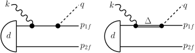
Figure 1: Nucleon- and $\Delta$-pole contributions to pion photoproduction on the deuteron.

However, this method fails for a resonance-like energy dependence which usually appears when certain degrees of freedom or states are projected out in favor of effective operators. This is the case in pion photoproduction where any realistic production operator contains resonance or pole contributions (see for example blomqvist ; DrH99 ) describing intermediate excitation of nucleon isobars. The problem, one encounters, can be illustrated already by the contribution of the nucleon-pole diagram to the production process on the two nucleon system depicted in Fig. 1, which is an essential ingredient in pion production. Projecting out the intermediate $NN$-system in time ordered perturbation theory, the corresponding amplitude has the following structure

$$O(E_{f})\propto\frac{1}{E_{f}+i\,\varepsilon-H_{0}}\,,\,$$ (10)

where $H_{0}$ denotes the free $NN$-hamiltonian. Recalling now the different steps in equation (4) and (6), and applying the LIT approach naively would mean to replace the energy $E_{f}$ appearing in the propagator by the full hamiltonian $H$ of the final $\pi NN$-system. This, however, does not make any sense, because $H_{0}$ and $H$ act on different particle systems. Also the method of treating the energy as a parameter does not work, because in this case the effective operator becomes singular and thus the Lorentz state is not normalizable any more.

The physical reason for the energy dependence of the contribution (10) is quite obvious because the intermediate $NN$-configuration has been projected out in favor of an effective operator. The same situation appears for the $\Delta$-resonance contribution in Fig. 1, which is also described by an effective, energy dependent operator. A way out of this dilemma is to enlarge the configuration space by including the previously projected-out states and thus avoiding the energy dependence of effective operators.

In the present case, where a meson is produced, we have to include configurations with different numbers of particles, i.e. we have to construct a genuine Fock space description. We will first consider a general Fock space ${\cal F}$ consisting of $N$ orthogonal subspaces labeled by $l$. The projectors $P_{l}$ onto these subspaces fulfil

$$\mathbb{1} = \sum_{l=1}^{N}P_{l}\,\quad\mbox{with}\quad P_{l}P_{m}=\delta_{lm}P_{l}\,.$$ (11)

The full Fock space hamiltonian $H=H_{0}+V$ consists of a kinetic part $H_{0}$ which is diagonal and an interaction $V_{lm}=P_{l}VP_{m}$, with $l,m\in\{1,...,N\}$, allowing transitions between the various subspaces. A transition operator, describing an electromagnetic process, is generally expressed by a hermitean current operator $j^{\mu}$ in ${\cal F}$, which does not contain any resonance-like energy dependence,

$$O=\sum_{l,m=1}^{N}\varepsilon_{\mu}j^{\mu}_{lm}\,\,\quad\mbox{with}\quad j^{\mu}_{lm}=P_{l}j^{\mu}P_{m}\,\,,$$ (12)

where $\varepsilon^{\mu}$ denotes the photon polarization vector. A remaining trivial energy dependence via current structures depending on the photon momentum can be handled by the parameter method.

In this Fock space, the LIT equation reads now

$$(H-\sigma)\mbox{$|\widetilde{\Psi}\rangle$}=O\mbox{$|\Psi\rangle$}\,,\,{\rm Im}\{\sigma\}\not=0\,.$$ (13)

To solve this equation we use the method of resolvents in analogy to standard scattering theory, i.e. we introduce

$${\cal G}_{0}(\sigma) = \frac{1}{\sigma-H_{0}}\,,\quad{\cal G}(\sigma)=\frac{1}{\sigma-H}\,.$$ (14)

Defining a conventional $T$-matrix by $T{\cal G}_{0}\equiv V{\cal G}$, one then obtains the following standard equations for the ${\cal G}$- and $T$-matrices

$${\cal G} = {\cal G}_{0}+{\cal G}_{0}T{\cal G}_{0}={\cal G}_{0}+{\cal G}_{0}V{\cal G}\,,$$ (15)

$$T = V+V{\cal G}_{0}T\,.$$ (16)

A formal solution of the LIT-equation can be written as

$$\mbox{$|\widetilde{\Psi}\rangle$}=-{\cal G}O\mbox{$|\Psi\rangle$}\,.$$ (17)

Since $O$ is regular and ${\rm Im}\{\sigma\}\not=0$ , the Lorentz state $\widetilde{\Psi}$ is normalizable like a bound-state.

4 Application to $\pi^{0}$-photoproduction via the excitation of the $\Delta$-resonance

As a test case, we will consider now $\pi^{0}$-photoproduction off the deuteron in the $\Delta$-region. Then ${\cal F}$ comprises besides $\pi^{0}NN$- also $NN$- and $N\Delta$-states, so that nucleon-pole as well as $\Delta$-pole contributions to the photoproduction process can be taken into account. Using a compact matrix notation with respect to the three projectors $P_{\pi}$, $P_{N}$ and $P_{\Delta}$ for the $\pi^{0}NN$, $NN$- and $N\Delta$-subspaces, respectively, we can cast kinetic and interaction parts of the hamiltonian $H=T+V$ into the following form

$$H_{0}=\left(\begin{matrix}T_{N}\\ &T_{\Delta}\\ &&T_{\pi}\end{matrix}\right)\,\,,\quad V=\left(\begin{matrix}V_{NN}&V_{N\Delta}&V_{N\pi}\\ V_{\Delta N}&V_{\Delta\Delta}&V_{\Delta\pi}\\ V_{\pi N}&V_{\pi\Delta}&V_{\pi\pi}\end{matrix}\right)\,\,.$$ (18)

Transitions between different subspaces are described by the non-diagonal matrix elements of $V$. For example, $V_{\pi N}$ contains the $\pi^{0}N$-vertex allowing transitions between the $NN$- and $\pi^{0}NN$-states. Since we only want to demonstrate the applicability of our approach and do not aim at a quantitative description of the data, we restrict the interaction solely to $V_{\Delta\pi}$ and $V_{NN}$, i.e. we use

$$V=\left(\begin{matrix}V_{NN}&0&0\\ 0&0&V_{\Delta\pi}\\ 0&V_{\pi\Delta}&0\end{matrix}\right)\,.$$ (19)

The parametrization of the $\Delta N\pi^{0}$-vertex $V_{\Delta\pi}$ is taken from PoS87 . As electromagnetic current we consider here solely the dominant M1-$N\Delta$-current $\boldsymbol{j}_{N\Delta}$

$$\boldsymbol{j}_{\Delta N}(\boldsymbol{k})\sim\frac{G_{M1}^{0\,\Delta N}}{2M_{N}}\,i\,\boldsymbol{\sigma}_{\Delta N}\times\boldsymbol{k}\,\,$$ (20)

with $\displaystyle{G_{M1}^{0\,\Delta N}=4.22}$. With these building blocks we can describe the dominant $\Delta$-pole contribution to photopionproduction. With the approximations (19) and (20), the $NN$-interaction $V_{NN}$ contributes solely to the deuteron ground-state. For reasons of simplicity, we have used a pure $S$-wave Yamaguchi potential Yam with modern parameters from Dress . For a shorter notation we label operators $A$ connecting the same subspace with only one index, i.e. $A_{ll}\equiv A_{l}$. The Lorentz state can then be written as (see Fig. 2)

$$-\mbox{$|\widetilde{\Psi}\rangle$} = {\cal G}O_{\Delta N}\mbox{$|\Psi\rangle$}=(\mathbb{1}_{\Delta}+{\cal G}_{0\pi}V_{\pi\Delta}){\cal G}_{\Delta}O_{\Delta N}\mbox{$|\Psi\rangle$}\,.$$ (21)

The resolvent ${\cal G}_{\Delta}$ fulfils the equation (see Fig. 3)

$${\cal G}_{\Delta} = {\cal G}_{0\Delta}+{\cal G}_{0\Delta}V_{\Delta\pi}{\cal G}_{0\pi}V_{\pi\Delta}{\cal G}_{\Delta}\,,$$ (22)

which allows one to rewrite the LIT into the following form

$$L=-\frac{1}{\sigma_{\rm I}}\,{\rm Im}\left\{\mbox{$\langle\Psi|$}O_{N\Delta}\,{\cal G}_{\Delta}\,O_{\Delta N}\mbox{$|\Psi\rangle$}\right\}\,.$$ (23)

$V_{\Delta}$ consists of a loop diagram (disconnected) and a genuine two-body one-pion exchange potential (connected), see Fig. 3. If the latter is neglected, we will refer to it as impulse approximation (IA) and denote the corresponding resolvent from here on as ${\cal G}^{\rm IA}_{\Delta}$. Therefore in impulse approximation $L^{\rm IA}$ is given by (23) where ${\cal G}_{\Delta}$ is replaced by

$${\cal G}^{\rm IA}_{\Delta}=\frac{1}{\sigma-T_{\Delta}-{\Sigma_{\Delta}(\sigma)}}\,,$$ (24)

with $\Sigma_{\Delta}$ as self-energy of the $\Delta$

$${\Sigma_{\Delta}(\sigma)=V_{\Delta\pi}{\cal G}_{0\pi}(\sigma)V_{\pi\Delta}|_{\rm disconnected}\,\,.}$$ (25)

5 Results

The result for $\pi^{0}$-photoproduction on the deuteron is shown in Fig. 4. Besides the IA according to (24) with a variable $\sigma$-dependent $\Delta$-mass, we have calculated in addition another IA with a static $\Delta$-mass ($M_{\Delta}=1232$ MeV) for a better comparison with the IA of schmidt96 . Considering the small model differences to schmidt96 the agreement is quite satisfactory. While the IA is calculated without a partial wave decomposition, it is needed for the $N\Delta$-interaction contribution generated by the one-pion exchange diagram in Fig. 3. In order to fulfil convergence, we took into account all channels with a total angular momentum $J\leq 5$ of the $N\Delta$-system. One readily notes that the $N\Delta$-interaction has a sizeable influence near threshold leading to an enhancement and is still moderate near the maximum resulting in a slight upward shift of the position and lowering of the absolute size by about 8 %. For a realistic description of the cross section in the $\Delta$-region one has to include besides non-resonant photoproduction contributions the neglected FSI, i.e. $NN$- and $\pi N$-interactions DaA03 .

In conclusion, we have demonstrated how to extend the LIT method when energy dependent effective operators are involved. It turns out that in such a case those states, which have been projected out in favor of effective operators, have to be included explicitly in an expanded Fock space. With respect to the specific process considered here as an example, pion photoproduction on the deuteron, it is obvious that in the future the present model has to be extended towards a more realistic description of this reaction. First of all, additional FSI as well as nonresonant Born contributions have to be included. Furthermore, since this method really pays-off for more complex systems with more than two nucleons, one has to consider meson-photoproduction on other light nuclei like ³He or ⁴He.

This work was supported by the Deutsche Forschungsgemeinschaft (SFB 443).

Figure 2: Diagrammatic representation of $\widetilde{\Psi}$ in eq. (21).

Figure 3: Diagrammatic representation of ${\cal G}_{\Delta}$ in eq. (22).

Figure 4: Total cross section of $\pi^{0}$-photoproduction on the deuteron. Notation of the curves: dashed: IA with constant $\Delta$-mass; dashed-dotted: IA using eq. (24); full: inclusion of $N\Delta$-interaction; dotted: IA according to schmidt96 (only resonance).

References

- (1) V.D. Efros, W. Leidemann, and G. Orlandini, Phys. Lett. B338 130 (1994).
- (2) S. Martinelli, H. Kamada, G. Orlandini, and W. Glöckle, Phys. Rev. C 52 1778 (1995).
- (3) S. Bacca, M. Marchisio, N. Barnea, W. Leidemann, and G. Orlandini, Phys. Rev Lett. 89, 052502 (2002).
- (4) S. Bacca, H. Arenhövel, N. Barnea, W. Leidemann, and G. Orlandini, Phys. Lett. B 603 159 (2004).
- (5) V.D. Efros, Sov. J. Nucl. Phys. 41 949 (1985).
- (6) A. La Piana, and W. Leidemann, Nucl. Phys. A677 423 (2000).
- (7) S. Quaglioni, W. Leidemann, G. Orlandini, N. Barnea, and V.D. Efros, Phys. Rev. C 69, 044002 (2004).
- (8) D. Gazit and N. Barnea, Phys. Rev. C 70, 048801 (2004).
- (9) J. M. Laget, Phys. Rep. 69, 1 (1981)
- (10) S. S. Kamalov, L. Tiator, and C. Bennhold, Phys. Rev. Lett. 75 1288 (1995).
- (11) W. Glöckle, The Quantum Mechanical Few-Body Problem, Springer (1983).
- (12) C. Reiß, W. Leidemann, G. Orlandini, and E.L. Tomusiak, Eur. Phys. J. A 17, 589 (2003).
- (13) N.M. Kroll and M.A. Ruderman, Phys. Rev. 93 233 (1954).
- (14) D. Andreasi, W. Leidemann, C. Reiß, and M. Schwamb, accepted for publication in Eur. Phys. J. A (2005); preprint nucl-th/0503033.
- (15) I. Blomqvist and J.M. Laget, Nucl. Phys. A280 405 (1977).
- (16) D. Drechsel, O. Hanstein, S. S. Kamalov, and L. Tiator, Nucl. Phys. A645 145 (1999).
- (17) H. Pöpping, P. U. Sauer, and X.-Z. Zang, Nucl. Phys. A474, 557 (1987).
- (18) Y. Yamaguchi, Phys. Rev. 95 1628 (1954).
- (19) E.T. Dressler, W.M. MacDonald, and J.S. O’Connell, Phys. Rev. C20 267 (1979).
- (20) R. Schmidt, H. Arenhövel, and P. Wilhelm, Z. Phys. A 355 421 (1996).
- (21) E. M. Darwish, H. Arenhövel, and M. Schwamb. Eur. Phys. J. A16 111 (2003).