Description of intermediate- and short-range $NN$ nuclear force within a covariant effective field theory

Abstract

The present paper is aimed to developing an effective field theory in the GeV region to describe consistently both elastic and inelastic $NN$-scattering in a fully covariant way. In this development we employ our novel $s$-channel mechanism of $NN$-interaction at intermediate and short ranges assuming a formation of the six-quark bag dressed with basic meson fields such as $\pi$, $\sigma$, $\rho$ and $\omega$ in the intermediate state. The peripheral part of the interaction is governed by $t$-channel one- and two-pion exchanges described fairly well by chiral perturbation theory. The $\sigma$-meson dressing should be especially important for the stabilization of the bag due to a high coupling constant of the $\sigma$-meson with the bag and also a strong interaction between the $\sigma$-field and space symmetric quark core $|\mathrm{s}^{6}[6]\rangle$. This stabilization of the intermediate dressed bag (which shifts the mass of the bag downward to $NN$ threshold) will be crucially important for the description of $\pi$, $2\pi$, $\rho$ and $\omega$-meson production in $NN$-collisions, and, in particular, for the correct description of $\pi^{0}$ production near threshold. So that, we expect that the results of the present work will lead to a deeper understanding the short- and intermediate-range nuclear forces and internucleon correlations in nuclei.

, and

1 Introduction: modern status of the theoretical description for the intermediate- and short-range $NN$ interaction

More than 50 years ago Hans Bethe has remarked about the nature of nucleon-nucleon in his famous review “What Holds the Nucleus Together?”: “…In the past quarter century physicists have devoted a huge amount of experimentation and mental labor to this problem – probably more man-hours than have been given to any other scientific question in the history of mankind …”. And this claim is still valid today. Despite of the enormous efforts of many labs, groups and personal researchers over the world during the last 50 years and despite of the great progress in experiments and fundamental theory provided by developments in QCD, we are still not having in our disposal a consistent and reliable dynamical theory for the $NN$-interaction at intermediate and especially at short distances, which can form a solid basis for the explanation of numerous precise experimental data in meson-production in $pp$, $pd$, …collisions, in few-body physics and in many two-proton photo-emission nuclear experiments, like $\mathrm{A}(\gamma,pp)$, $\mathrm{A}(e,e^{\prime}pN)$ etc., at rather high momentum transfer.

We enumerate here some of basic points where the conventional description of the short-range $NN$-interaction in terms of meson exchanges (e.g. $\sigma$, $\rho$, $\omega$, $\rho-\pi$, $\omega-\pi$ etc.) fails or looks to be quite inconsistent. First of all, the value of the $\omega NN$ coupling constant (which is responsible for the short-range $NN$ repulsion and the spin-orbit splitting) accepted in all OBE-models turns out to be in the range $g^{2}_{\omega NN}/4\pi=13.6-20$ which is much larger than the respective SU(3) value ($\sim 5$) while all other coupling constants used in OBE-models are in a good agreement with the respective SU(3) predictions. Another evident inconsistency is that almost all meson-exchange nucleon-nucleon models use a too high value for the tensor-to-vector $\rho$-meson coupling to the nucleon, $\kappa_{\rho}\approx 6-7$. At the same time, an analysis of the data on $\pi N$ scattering yields a much more modest value, $\kappa_{\rho}\approx 1-3$ for this parameter (see, e.g. [1]). Thus the short-ranged central and tensor nucleon-nucleon forces in boson-exchange models are enhanced ”by hand” to reproduce the experimental $NN$ phase shifts.

Another fundamental difficulty in the traditional OBE-approach, also tightly related to the short-range nucleon-nucleon interaction, are the very large values of cut-off parameters $\Lambda_{\pi NN}$, $\Lambda_{\pi N\Delta}$, …in meson-baryon vertices, which are responsible for short-range limit of the $NN$-interaction. In fact, the values of $\Lambda_{\pi NN}$, $\Lambda_{\rho NN}$ etc. accepted in traditional OBE-models ($\sim 1.5-2$ GeV) are at least three times larger than those derived from any dedicated experiments (e.g. from $\pi N$ scattering), or from all fundamental theories ($\sim 0.5-0.7$ GeV). Moreover, the values of $\Lambda_{\pi NN}$ or $\Lambda_{\rho NN}$ necessary to fit the charged pion production in $pp$-collision is strongly different from those values needed to fit the elastic $pp$-scattering. And those both values are different from respective values which are adopted in $3N$-force operator to fit the $3N$ binding energy within $2N$- and $3N$-force models driven by one-boson exchange [2, 3, 4, 5].

Figure 1: Average $\@@nuc{3}{He}(e,e^{\prime}pp)$ cross section as a function of the missing momentum $p_{m}$ for the data measured in kinematic settings LQA and LQV (for the explanation see the text of Ref. [7]) and the (energy, momentum) transfer values ($\omega,q$)=(220 MeV, 305 MeV/c). The solid and dashed lines represent the results of calculations with a one-body current operator and including MECs, respectively, using the Bonn-B $NN$ potential.

Figure 2: Average $\@@nuc{3}{He}(e,e^{\prime}pp)$ cross section as a function of the energy transfer $\omega$ at the value of momentum transfer $q=375$ MeV/c and $50<p_{m}<100$ MeV/c (left) and $200<p_{m}<300$ MeV/c (right). The crosses give the experimental data while the curves represent calculations with a one-body current only (solid), including MECs (dashed) and including MECs and static isobar currents (dot-dashed).

A direct consequence of the improper treatment for the short-range nuclear force and respective short-range two-nucleon correlations in nuclei is a quite serious disagreements between the predictions of most realistic modern few-body theories and data observed in a few key e.-m. experiments like $\mathrm{A}(e,e^{\prime}pp)$, $\mathrm{A}(e,e^{\prime}pn)$ etc. at rather high momentum and energy transfers [6]. To illustrate the current situation in this field we present in Figs. 2 and 2 (taken from Ref. [7]) the comparison between the most elaborated modern calculations for $3N$-system (both in bound state and continuum) which include also the respective MEC-contributions [8] and the results of recent experiments at NIKHEF on $\@@nuc{3}{He}(e,e^{\prime}pp)n$ reaction.

It is clearly seen from the comparison between theoretical and experimental results that the underlying mechanism of the reaction should be quite different as compared to that assumed in the existing theoretical approach (because the energy and momentum dependence derived from the theory have opposite trends than the experiments showing – see Fig. 2). A similar disagreement has also been observed in electromagnetic knock-out of a $pn$-pair from $\@@nuc{3}{He}$ [9] in the Mainz experiments. So one can expect a quite different mechanism for such reactions at rather high momentum transfers as compared to that underlying the OBE-picture of $2N$ and $3N$ interactions.

The key problem in a consistent theoretical description for such experiments is that the large incident momentum of a high-energy projectile has to be shared among several nucleons in nuclei, which requires a very strong short-range correlation of nucleons [10]. But the conventional picture of the correlations induced by the $t$-channel meson exchanges can transfer the high momentum only with high values of cut-off parameters $\Lambda$, or, alternatively, by incorporation of the numerous diagrams with multiple rescatterings in intermediate state [11], which are out of the control.

In the last decade, numerous attempts have been made to describe the intermediate and short-range $NN$ interaction within the framework of a cluster quark model employing the Resonating Group Method (RGM) approach [12, 13, 14, 15]. However all these attempts were only partially successful and unable to extend the energy range much larger than 300–400 MeV. Another serious problem with these QCD-inspired approaches is their inability to describe consistently the inelastic processes, e.g. the one- or two-pion productions. They focused only on the elastic $NN$ scattering at rather low energies. Thus we have now “on the market” two extreme types of models for the short and intermediate range $NN$ interaction: either the traditional OBE-type models which do not include any quarks, or the quark-motivated models which include the mesons only as the carriers of $qq$ interaction [12], i.e. with no explicit mesonic degrees of freedom. Thus, with such a limited basis the quark models immediately meet serious problems in the description of meson production in $NN$ collisions (which do require the incorporation of mesonic degrees of freedom in an explicit form).

After the well-known work of Weinberg [16] the effective field theory (EFT) approach became very popular and has been applied to the $NN$ interaction and related phenomena in two forms: (i) in the “pionless” form which generalises somehow (in field-theory language) the effective range expansion [17] and (ii) in the form of Chiral Perturbation Theory (ChPT). In both directions great progress has been made and full calculations up to high orders are now feasible. Within the framework of ChPT the calculations have been performed [18, 19] (see also [20]) for $NN$ elastic scattering with energies up to 290 MeV (in lab. system) and for deuteron properties. The authors [18] used the ChPT expansion up to fourth order (i.e. $\mathrm{N}^{3}\mathrm{LO}$) and have derived the respective $NN$-potential which leads to the same quality of fit for the $NN$ phase shifts (with $\chi^{2}\sim 1$) as for the best modern phenomenological $NN$-potentials. For this fit some 29 free parameters has been employed, 26 of them being related to parametrization of contact terms (in $L\leq 2$). These contact terms, however, are out of the control by chiral theory and thus the description of short-range interaction is still on a purely phenomenological level.

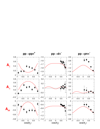
Figure 3: Comparison of the model predictions (see the Ref. [22]) to the data ($pp\rightarrow pp\pi^{0}$) taken from Ref. [21], ($pp\rightarrow d\pi^{+}$) Ref. [23] and ($pp\rightarrow pn\pi^{+}$) Ref. [24].

On the other hand, recent very powerful efforts of the Juelich group to describe quantitatively the very abundant and precise new data on the neutral pion production cross sections and analyzing powers in $\pol{p}\pol{p}$-collisions obtained in IUCF [21] have revealed a rather strong disagreement between well developed theory based on the meson-exchange approach and the polarization observables (see Fig. 3) [22]. This means that the traditional models still fail to describe the $\pi^{0}$-production in $pp$-collisions (especially for the spin observables). There are also quite serious problems in the description of two-pion production in $pp$-collisions found in recent experiments at Uppsala [25]. Here the main focus is on the simultaneous description of $\pi^{+}\pi^{-}$, $\pi^{0}\pi^{0}$ and $\pi^{+}\pi^{0}$ pair production. While the existing theory is able to predict the data in one channel, e.g. in the $\pi^{+}\pi^{-}$ channel, it fails to give a reasonable description in the other two channels (see Fig. 4). So, the existing theory seems not to include some important contribution(s) in the two-pion production sector.

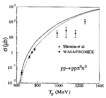
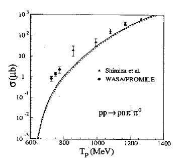
Figure 4: The total cross sections for the two-pion production $pp\rightarrow pp\pi^{0}\pi^{0}$ and $pp\rightarrow pn\pi^{0}\pi^{+}$ (quoted from Ref. [25]) shown together with the previously existing data in the intermediate energy region [26]. The curves represent theoretical predictions [27].

All these problems are tightly interrelated to the short- and intermediate-range $NN$ interaction. So, the understanding of this part of $NN$-interaction should be essentially improved. It is worth to add here that some interesting new proposal dedicated to the experimental and theoretical study for short-range $pp$ correlations in $\@@nuc{3}{He}$ and other light nuclei have been elaborated very recently by a team in the US [28]. But in their project the authors avoided any reference to microscopic or field-theory approaches and employed only some phenomenological estimations based on $pp$ scattering in the high-energy region.

On the other hand, the short-range $NN$ correlations are very crucial for our understanding the nuclear properties at moderate and high momentum transfer and more deep insight into phase transitions in nuclear matter. It should be stressed here while the existing theory can treat the averaged nuclear properties like single-particle momentum distribution on the quantitative level it meets serious problems when explaining the two-body short-range correlations even for the lightest nuclei like $\@@nuc{3}{He}$, where we can treat now both bound states and also the three-nucleon continuum fully consistently (i.e. with complete account of FSI and rescattering terms). Thus all the above facts (and also other arguments omitted here) and experimental findings have motivated us to develop some alternative approach for the intermediate- and short-range nucleon-nucleon force and alternative mechanisms for single- and two-meson production and also for short-range correlations in nuclei.

The present study is devoted to developing an alternative and new way for the treatment of the intermediate- and short-range correlations [3, 29, 30]. This novel approach starts with an important observation that the $t$-channel nucleon-nucleon interaction induced by two-pion exchange with full account of $2\pi$ correlation in $I=J=0$ state (i.e. in the $\sigma$ meson channel), being treated consistently, leads inevitably to strong short-range repulsion and very weak intermediate-range attraction [31, 32, 33] instead of the strong attraction induced by the conventional $\sigma$ meson exchange in OBE-models where the $\sigma$ is treated as a stable particle [34]. This amazing result has been obtained recently by two independent methods [32, 33] and thus looks to be established rather reliably. Moreover, in the latter work [33] it was found that even the $NN$ spin-orbit force induced by scalar $2\pi$-exchange is almost totally repulsive, i.e. it is in sharp contrast to that which is required by the fit to $NN$ phase shifts. So, we need some other general source for intermediate-range strong attraction and the short-range repulsion for the central $NN$ force and also an another source for the strong attractive spin-orbital $NN$ interaction.

The new force model proposed recently by two groups jointly: the Moscow State University group and the Tübingen University group [3, 29, 30, 35], treats the intermediate- and short-range $NN$-interaction as that proceeding through an intermediate dressed six-quark bag (i.e. via $s$-channel mechanism):

$$NN\rightarrow(6q+\mathrm{meson\ fields})\rightarrow NN,$$

where the dressing by the meson fields (mainly through the $\sigma$-field) surrounding the dense six-quark core strongly stabilizes the $6q$-bag and shifts its mass downward to the $NN$ threshold. The physical pattern underlying this new $s$-channel mechanism can be shortly outlined as follows [35]. Due to a strong attraction of the $\sigma$-meson to the quarks in the $|\mathrm{s}^{6}[6]\rangle$ configuration and spherical symmetry of the $\mathrm{s}^{6}$ six-quark bag, the $\sigma$-field will compress somehow the bag. This bag compression may induce very short-range scalar diquark correlations in the bag and enhances further the quark-meson interaction. All these attractive effects will compensate completely the energy losses originated from $\sigma$-meson generation and rather high kinetic energy of quarks in the bag. So the net result of this interplay has been estimated to be strongly attractive. Then we employed the quark-meson microscopic model [29, 30] to estimate these effects and to construct the respective new model for the $NN$ interaction at short ranges. Our extensive tests have demonstrated [30, 35, 36, 37] that this model works very well and makes it possible to explain many long-standing puzzles in the field, e.g. it uses the OPE terms with proper cut-off parameters $\Lambda\sim 0.5$ GeV. The new model predicts also the appearance of a strong three-nucleon scalar force induced by $\sigma$-exchange between the dressed bag and the third nucleon.

To study the effects of the new $3N$ scalar force when calculating the properties of $\@@nuc{3}{H}$ and $\@@nuc{3}{He}$ nuclei, we have developed [36, 37] some multi-component formalism which made it possible to include both nucleonic and dibaryon components into $3N$ wave functions. It has been found [36] the latter components in $3N$ wave function has a quite noticeable weight ($\sim 10\%$ or even higher) and these contribute very essentially to the total $3N$ binding energy. Thus the interplay between two-body and three-body force contributions peculiar to the conventional force models is changed drastically in the new approach. However, despite of this, we were still able to describe fully quantitatively, with no adjustable parameters, the basic static properties of $\@@nuc{3}{H}$ and $\@@nuc{3}{He}$ nuclei, especially the Coulomb displacement energy $E_{B}({}\@@nuc{3}{H})-E_{B}({}\@@nuc{3}{He})$ which was a long-standing puzzle in the field. Thus we can summarize here that albeit the new force model predicts some novel features of nuclear force it leads, at least, for static observables, largely to the same $3N$ observables as for other modern approaches like CD-Bonn $2N+3N$ UIX or TM forces. However many other effects in strong or electroweak interaction phenomena will be described in fully different manner with the new force model.

In previous versions of the model [30], we extensively employed the semi-relativistic quark-meson microscopic model and $\sigma$-meson dressing and have fitted the lower partial $NN$ phase shifts with the model up to 1 GeV. However, in order to work reliably in the range 1–3 GeV we need a consistent fully relativistic approach.

Another important application of the new force model was a treatment of short-range $N\Delta$ interaction within the same dressed bag model [38]. This part of $N\Delta$ interaction is at the moment still poorly known, however it can be crucially important in the description of numerous processes in two- and few-nucleon systems going through $\Delta$-isobar current and accompanied by a large momentum transfer, like one- or two-pion photoproduction $d(\gamma,\pi^{+})$, $d(e,e^{\prime}\pi^{+}\pi^{-})$ etc. In our new field theoretical approach the $N\Delta$ and $\Delta\Delta$ channels are considered on the same footing as $NN$ channel by calculating the respective $N\Delta$ and $\Delta\Delta$ loops of the dressed dibaryon [39].

On the other hand, the formalism developed makes it possible, in general, to treat the elastic and inelastic channels in a unified way (see the subsequent section of the article). The only possible way that meets the above general requirements which the present authors can presently imagine is a fully covariant field-theoretical approach. Effective field-theory approaches became very popular in this field in last decade.

Such an effective field approach is ideally suited for our purposes because it includes in an absolutely natural manner the relativistic formalism and the processes (in intermediate and final states) with generation of other particles (mesons, isobars etc.). It can deal also quite naturally with meson and baryon loops in the intermediate states.

Thus we propose in the current work to develop a unified effective field theoretical approach to treat intermediate- and short-range $NN$-interaction at low and intermediate energies of 1–3 GeV jointly with description of meson production processes at $pp$ and $pn$ collisions. The clear distinction of the present force model from the existing ones in this aspect is the appearance of new (dressed) dibaryon components in all nuclei with quite significant weight $\sim 5-10\%$. This component can absorb, contrary to the conventional single-nucleon picture, a large momentum and energy. So, many processes associated, e.g. with high momentum transfer, can proceed easily through this new dibaryon component, the latter being excited by external probe can produce e.g. a few mesons, or an isobar etc. And these production processes through the intermediate dressed dibaryon should have much a higher probability than the corresponding processes by absorption on one nucleon or on a meson-exchange current. Our first calculations made within the framework of this approach to treat some electromagnetic processes in $2N$ and $3N$ systems have lead to quite promising results [36, 37, 40].

The structure of the paper is as follows. In Section 2, we explain the new physical model for intermediate and short-range $NN$ interaction. In Section 3, an effective field-theoretical approach is developed, which describes in the field-theoretical language the above physical model with $s$-channel dibaryon generation. Section 4 is devoted to derivation of a relativistic $NN$-potential using the formalism developed above. The semi-phenomenological nonrelativistic model proposed by our joint group previously is compared with the present treatment. In Section 5, we dwell briefly on a generalization of our approach to other hadronic processes like single- and two-meson production in $pp$-collisions. In Conclusion, we summarize the content of the work.

2 Physical model for the intermediate- and short-range $NN$ force

Here we will outline a multiquark model for the intermediate dressed dibaryon in $s$-channel, whose formation is assumed to be responsible in our approach for intermediate- and short-range $NN$ interaction.

We start with an observation done a decade ago [41] that from two possible space symmetries, viz. $[3]_{x}\otimes[3]_{x}=[6]_{x}\oplus[42]_{x}$, the $|\mathrm{s}^{6}[6]_{x}\rangle$-component has comparable projections onto three possible two-cluster components, viz. $|NN\rangle,|\Delta\Delta\rangle$ and $|CC\rangle$, while the second possible component $|\mathrm{s}^{4}\mathrm{p}^{2}[42]_{x}\rangle$, which corresponds to the $2\hbar\Omega$ excited six-quark configuration (more exactly a coherent sum of many such components), has a large projection onto the $|NN\rangle$ channel only. Thus, the fully symmetric part of the total six-quark wave function $|\mathrm{s}^{6}[6]_{x}\rangle$ can be identified with the bag-like structure while the mixed symmetry part $|\mathrm{s}^{4}\mathrm{p}^{2}[42]_{x}\rangle$ should be associated with the cluster-like $|NN\rangle$ component. Hence, from the six-quark symmetry point of view the $2\hbar\Omega$-excited six-quark part corresponds to the proper initial $NN$ channel while the ground $|\mathrm{s}^{6}[6]_{x}\rangle$ part includes mainly the intermediate bag-like components. Therefore the whole $s$-channel process going through the intermediate dressed dibaryon can be represented by the following chain of steps:

1. Fusion of two three-quark nucleon clusters into $2\hbar\Omega$ excited six-quark system with the space symmetry $|\mathrm{s}^{4}\mathrm{p}^{2}[42]_{x}\rangle$.

2. Emission of two $S$-wave pions from the excited mixed symmetry bag with subsequent formation of the scalar isoscalar $\sigma$-meson due to very strong correlation of these two $S$-wave pions: $|\mathrm{s}^{4}\mathrm{p}^{2}[42]_{x}\rangle\Rightarrow|\mathrm{s}^{6}\rangle+(\pi\pi)_{J=I=0}$.

3. Generation of the spherical dense six-quark bag $|\mathrm{s}^{6}+\sigma\rangle$ in which the spherical core is surrounded by strong scalar $\sigma$-field that compresses the quark bag due to strong attraction between $\sigma$-field and quarks.

In this new phase, one has two very important features characterizing the six-quark dynamics of the bag:

• partial restoration of the chiral symmetry, that leads to strong reduction in both $\sigma$-meson and constituent quark masses;

• essential enhancement of diquark correlations in the bag due to the bag compression. This enhancement should lead to additional energy gain in the process.

These two strong effects lead to a strong effective attraction in $NN$-channel at intermediate range. And this two-stage complicated mechanism replaces in our approach the simple $t$-channel $\sigma$-exchange in conventional OBE-models (which is invalid as has been proved by recent studies [32, 33] – see the Introduction) and is the origin for intermediate range $NN$-attraction.

However, this dressed bag state, being singlet in color space, has still a large overlap with the $NN$-channel, so that this state can decay fast back into the initial $NN$-channel. Hence, this intermediate dibaryon has a large width ($\sim 300-400$ MeV) and thus cannot be visualized as a resonance-like bump in $NN$ phase shifts or cross sections. Our previous papers [3, 29, 30] have demonstrated that this two-stage mechanism is quite able to explain with reasonable $\sigma qq$ and $\pi qq$ coupling constants $NN$ phase shifts in low partial waves up to 1 GeV. So that, quite similar to the nucleon dressing by a pion field, the dibaryon is dressed mainly by the scalar-isoscalar $\sigma$-field and the physical dibaryon should exist partially in the bare state and in the dressed state.

Resorting to a diquark language for description of the $NN\rightarrow\mathrm{DBS}$ (the dressed bag state) transition, one can assume that two unpaired quarks from both nucleons form a diquark pair (of scalar or axial-vector type) and thus, the intermediate stage in the transition is a state composed from three diquarks. Then such a three-diquark state gets dressed further with the $\sigma$-field that squeezes the bag. As a consequence, it can become favourable for diquarks to condense [43, 44, 45] at large energies. At the same time, the chiral symmetry gets partially restored, i.e. we are faced to a phase transition from the usual chiral-broken phase to the so-called color superconducting phase. In the present study, we are, of course, far from the regime of color superconductivity but the quark-quark correlations can still play a significant role already in low energy physics. In some way diquarks can serve as useful constituents and building blocks in investigating the properties of multi-quark systems [46]. Anyway, the generation of the $\sigma$-field in the symmetric $6q$-bag leads to a large energy gain and the physical mass of the dressed bag shifts strongly downwards. Effectively it corresponds to an appearance of a strong attractive force in the $NN$-channel.

Another important issue in the suggested mechanism for $NN\rightarrow\mathrm{DBS}$ transition is a domination of the excited mixed symmetry $|\mathrm{s}^{4}\mathrm{p}^{2}[42],LSI\rangle$ in the initial stage of the transition, so that the resulting $NN$-wave function has a nodal structure. That the $2\hbar\Omega$ excited mixed symmetry state dominates in the $NN$-wave function over a fully symmetric non-excited $|\mathrm{s}^{6}[6]\rangle$ configuration can be argued from various points of view. One argument is related to the specific spin-flavor nature of $qq$ interaction in the Goldstone-boson-exchange model [47]. However, in this model for the $qq$ force, both configurations lie rather high in energy, so that the effective $NN$-interaction in both symmetries corresponds to repulsion. The second argument is that the $\sigma$-dressing of the mixed symmetry bag: $|\mathrm{s}^{4}\mathrm{p}^{2}[42]\rangle\rightarrow|\mathrm{s}^{6}[6]+\sigma\rangle$ leads to much stronger energy shift of the bare initial $6q$-configuration than the respective shift of the symmetric state: $|\mathrm{s}^{6}[6]\rangle\rightarrow|\mathrm{s}^{6}[6]+\sigma\rangle$, because the latter process is in close analogy with the Lamb shift (due to interaction of quarks in the bag with vacuum fluctuations of the scalar field around the bag) while in the first process the $\sigma$-field is generated via a real deexcitation of two $\mathrm{p}$-shell quarks and their transition to the $\mathrm{s}$-orbit. The next section is devoted to the more formal and strict formulation of this qualitative pattern in terms of a covariant effective field theory.

3 Effective field theory with dibaryonic degrees of freedom for description of intermediate- and short-range $NN$ interaction

We are aiming to develop a consistent covariant field-theoretical description for the dibaryon model of nuclear forces, which allows us to go up to the intermediate energy region 1–3 GeV inaccessible to ChPT. This approach leads to the important modification of the force model: there arises a consistent scheme for the dressing of $6q$-bag in terms of effective field theory. Here the additional account of mesonic degrees of freedom in the DBS leads to an addition of corresponding loops in the complete polarization operator of the dibaryon, instead of a total replacement of the vertices in the transition $NN\rightarrow D+m$ ($m=\pi,\sigma,\omega,...$), (as was in our previous version of the model [30] and was described briefly in the preceding Section), see Fig. 5.

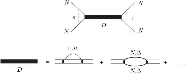
Figure 5: The graph in the first row illustrates the $s$-channel $NN$ interaction through the intermediate dressed dibaryon $D$ (the peripheral one-pion exchanges are also shown). The graphs in the second row illustrate some possible diagrams for the dibaryon dressing.

It is important to stress that such a field theoretical picture allows to carry out a natural matching between the field theory approach at low-energies (where ChPT is fully applicable) and the high energy region. In both regions one can now formulate a field theoretical language. In such an approach, the peripheral, i.e. the “external” part of $NN$-interaction is described by the conventional $\pi$- and $2\pi$-exchanges in the $t$-channel while the intermediate and short range interaction is described via generation of an intermediate dressed dibaryon which can be represented as a color quantum string able to vibrate and rotate. In the present model the intermediate dibaryon is produced by the color exchange between two quarks belonging to different nucleons with subsequent formation of a double string (possibly with diquark clusterization due to a strong $\sigma$-field generated on later stages of the process). The schematic evolution for this process is depicted in Fig. 6. To be more specific, we assume when the two quarks belonging to different $3q$-clusters interact and exchange a color, this can lead to the formation of either a nonconfined six-quark state (i.e. $NN$, $N\Delta$, etc.) or a confined $6q$-state locking by a hexagon-type string [39]. The first non-resonance process is, in fact, analogous in action to conventional meson exchange, while the second leads to formation of a hidden color $CC$-state. In diquark language, the first mechanism can be represented by the diagram with two interacting quarks forming a color representation ${\bf 6}$ of SU(3) group, because the one-gluon exchange or instanton induced interaction between quarks in this channel is repulsive. But if two interacting quarks form the system in a $\overline{\bf 3}$ color representation, the attractive correlations may lead to patching the quarks and as a consequence to the diquark formation. In this latter case, the dibaryon can be modeled as a system of three diquarks connected by Y-type string.

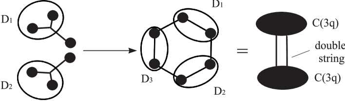
Figure 6: Possible mechanism of dibaryon formation. $D_{i}$ means that there are possible diquark correlations in dibaryon.

3.1 General formalism

Because the value of quark radius of a nucleon is around 0.6 fm and the interaction between quarks can proceed also at the peripheral regions of both nucleons, the size of the intermediate dibaryon can be around 1 fm, so that the dibaryon cannot be considered as a point-like object. Thus, the transition amplitude $NN\rightarrow D(CC)\rightarrow NN$ must be described through the non-local Lagrangian density:

$$M_{fi}=\mathrm{i}\langle 4,3|\mathrm{T}\left[e^{\mathrm{i}\int\d x\d x^{\prime}\mathcal{L}_{\mathrm{int}}(x,x^{\prime})}\right]|2,1\rangle-\mathrm{i}\langle 4,3|\mathrm{I}|2,1\rangle.$$ (1)

Here T means time-ordering while the bra and ket $|2,1\rangle$ and $\langle 4,3|$ relates to the initial and final nucleons with 4-momenta $p_{2},p_{1}$ and $p_{4},p_{3}$ respectively. The second term in (1), where $\mathrm{I}$ is the unit matrix, corresponds to the propagation of noninteracting nucleons and thus must be subtracted.

The nonlocal Lagrangian density in Eq. (1) corresponding to transition from the two-nucleon to a bare dibaryon state, and the subsequent dibaryon dressing can be written in the form:

$$\mathcal{L}_{\mathrm{int}}(x_{1},x_{2})=\mathcal{L}_{DN}+\mathcal{L}_{Dm},$$ (2)

where the Lagrangian

$$\mathcal{L}_{DN}=\widetilde{N}(x_{2})\{\Psi(x_{1},x_{2})V_{0}(x_{1}-x_{2})+\gamma_{5}\gamma^{\mu}\Psi_{\mu}(x_{1},x_{2})V_{1}(x_{1}-x_{2})\}N(x_{1})+\mathrm{h.c.}$$ (3)

is odd in dibaryon field operators $\Psi$ and $\Psi_{\mu}$, and the Lagrangian $\mathcal{L}_{Dm}$ describing the interaction of $6q$-bag with its meson cloud, is even in $\Psi$’s. The function $\Psi(x_{1},x_{2})$ describes the dibaryon with spin $S=0$, while $\Psi_{\mu}(x_{1},x_{2})$ corresponds to the $S=1$ dibaryon (in both cases the isospin is assumed to have the value $I=0$, for the case of isospin $I=1$ we should make a replacement $\Psi\rightarrow\vec{\tau}\vec{\Psi}$ in (2)). The bispinor $\widetilde{N}\equiv N^{T}C^{-1}\gamma_{5}\mathrm{i}\tau_{2}$ has the same transformation properties as the Dirac-conjugated nucleon-field operator $\overline{N}=N^{\dagger}\gamma_{0}$ in the Lorentz and isospin groups, $C=\mathrm{i}\gamma_{2}\gamma_{0}$ is the charge-conjugation operator, $\tau_{2}$ is a Pauli matrix, and $N^{T}$ stands for a transposed matrix. We use the notation and definitions borrowed from Ref. [48].

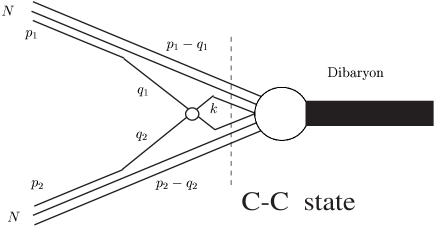
Figure 7: The vertex for two-nucleon-to-dibaryon transition when two quark, belonging to different nucleons, interact with each other with subsequent formation of hidden color $CC$-state (or dibaryon) bound by double string.

The interaction $V(x_{1}-x_{2})$ related to the transition vertex $NN\rightarrow D$ can be illustrated by the graph shown in Fig. 7. This interaction can be found, in general, from the quark-microscopic model, e.g. assuming a diquark substructure of the dibaryon. But, since in this work, we are interesting in developing a general effective field-theory approach to the dynamics of the intermediate dressed dibaryon we will ignore any details of quark substructure of the dibaryon. So that, the potential $V$ is taken from the overlap of the inner nucleonic wave functions (we postpone more elaborated calculation of this transition to the near future):

$$V(x)=g\int\d^{4}yf_{N}(y+x/2;p_{1})f_{N}(y-x/2;p_{2}),$$ (4)

where we choose for the $f_{N}$ the covariant harmonic oscillator wavefunction:

$$f_{N}(x;p)=\frac{\alpha}{\pi}\exp{\left[\frac{\alpha}{2}(x^{2}-\frac{2(xp)^{2}}{m_{N}^{2}})\right]},$$ (5)

$g$ is an effective coupling parameter and $m_{N}$ denotes the nucleon mass. In non-relativistic limit

$$f_{N}(x,p)\approx\frac{\alpha}{\pi}\exp{[-\alpha(x_{0}^{2}+{\bf x}^{2})/2]},$$ (6)

so we get a covariant form for $V(x)$:

$$V(x)=g\exp{\left[\frac{\alpha}{4}(x^{2}-\frac{2(xP)^{2}}{m_{N}^{2}})\right]},$$ (7)

where $P=p_{1}+p_{2}$ is the c.m. 4-momentum of two nucleons.

From Eqs. (1) and (3), it is evident that the transition amplitude must be even in dibaryon field operator and at least of the second order in interaction with a nucleon current. As a result, one has the following expression for $M_{fi}$ (in $I=0$ channel):

$$M_{fi}=\frac{1}{2!}\sum_{S}\int\d^{4}x_{1}\d^{4}x_{2}\d^{4}x_{3}\d^{4}x_{4}\langle 4,3|\overline{N}(x_{4})\Gamma_{S}^{\dagger}\overline{\widetilde{N}}(x_{3})\times\\ \times\mathcal{G}^{S}(x_{3},x_{4};x_{1},x_{2})\widetilde{N}(x_{1})\Gamma_{S}N(x_{2})|2,1\rangle V_{S}(x_{1}-x_{2})V_{S}(x_{3}-x_{4}),$$ (8)

where $\mathcal{G}^{S}(x_{3},x_{4};x_{1},x_{2})$ is an exact dibaryon propagator that takes into account the dressing of the dibaryon with meson fields. The vertices $\Gamma_{S}$ are equal:

$$\Gamma_{S}=\Biggl{\{}\begin{array}[]{c}1,\ \ \ \ \ \ S=0,\\ \gamma_{5}\gamma_{\mu},\ \ S=1.\end{array}$$ (9)

The dressed dibaryon propagator is found by solving the respective Dyson equation

$$\mathcal{G}^{S}(x_{3},x_{4};x_{1},x_{2})=G^{S}(x_{3},x_{4};x_{1},x_{2})+\\ \int\d^{4}x_{1}^{\prime}\d^{4}x_{2}^{\prime}\d^{4}x_{3}^{\prime}\d^{4}x_{4}^{\prime}G^{S}(x_{3},x_{4};x_{3}^{\prime},x_{4}^{\prime})\Pi^{S}(x_{3}^{\prime},x_{4}^{\prime};x_{1}^{\prime},x_{2}^{\prime})\mathcal{G}^{S}(x_{1}^{\prime},x_{2}^{\prime};x_{1},x_{2}),$$ (10)

where

$$G^{S}=-\mathrm{i}\langle 0|\mathrm{T}_{X,X^{\prime}}[\Psi^{S}(x_{3},x_{4})\Psi^{S}(x_{1},x_{2})]|0\rangle$$ (11)

is a bare dibaryon propagator and $\Pi^{S}$ stands for a polarization operator of the dibaryon. Here, the time-ordering is performed with respect to the coordinates $X$ and $X^{\prime}$ of the dibaryon center of mass. It is worth to note that the T-ordering on the coordinates (of the two color clusters) $x_{3},x_{4}$ and $x_{1},x_{2}$ in amplitude $M_{fi}$ corresponds only to the positive and negative signs for the time-like components of the relative coordinates $x=x_{1}-x_{2}$ and $x^{\prime}=x_{3}-x_{4}$ in the integration over $x_{i}$ ($i=1..4$), while the mixed ordering, for example, on the coordinates $x_{1},x_{3}$ and $x_{2},x_{4}$ results in two types of exchange interaction displayed in Fig. 8. The first graph describes the (resonance-like) $s$-channel exchange by the dibaryon whereas the second graph describes non-resonance $t$- and $u$-channel exchanges by an exotic dibaryon (which corresponds to a heavy $N\overline{N}$-meson). This exotic contribution is omitted in Eq. (8) and will be further neglected.

Figure 8: Diagrams representing the amplitude in Eq. (8). The first diagram corresponds to $s$-channel dibaryon exchange, while the second diagram describes the $u$- or $t$-channel exchange of a heavy $\overline{N}N$ meson having an exotic $3\overline{q}3q$ structure.

3.2 Dibaryon wavefunctions

We consider the dibaryon wavefunctions as a convolution of orbital and total spin parts: $\Psi(x_{1},x_{2})=\Phi(x;P)\otimes S(X;P)$, where the orbital part $\Phi(x;P)$ is taken as a superposition of covariant harmonic oscillator (CHO) eigenfunctions $f(x;P)$ (see below). Although there is presently no direct connection between the CHO-formalism and QCD, its application appears quite successful in describing the baryon spectra and the systematics of $\overline{q}q$ meson states [49]; in addition, it leads to hadron form factors whose behavior agrees well with experimental data. As for the microscopic basis of the CHO-functions one should note, that these eigenfunctions are closely related to the solution of the Dirac equation with a linear vector potential [50] which corresponds to a string-like interaction (between two colored clusters). The total spin wavefunctions $S(X;P)$ satisfy to the standard Klein–Gordon equation:

$$\left(\partial^{2}/\partial X^{2}_{\mu}+M_{N_{e}}^{2}\right)S(X;P)=0,$$ (12)

while the $f(x;P)$ is a tensor of rank $N_{e}$ ($N_{e}$ is the number of excitation quanta of the string) in the space $O(3,1)_{\mathrm{Lorentz}}$ and satisfies to the equation:

$$\mathcal{M}^{2}(x_{\mu},\partial/\partial x_{\mu})f(x;P)=M_{N_{e}}^{2}f(x;P).$$ (13)

with the mass operator squared is defined as

$$\mathcal{M}^{2}\equiv d\left(\frac{1}{2\mu}\frac{\partial^{2}}{\partial x^{2}_{\mu}}+U_{\mathrm{conf}}+U_{\mathrm{pert.QCD}}\right),$$ (14)

here $d=2(m_{1}+m_{2})$, $\mu=m_{1}m_{2}/(m_{1}+m_{2})$ and $m_{i}$ are kinematical masses of $3q(C)$ clusters on the ends of the string. $U_{\mathrm{conf}}$ is defined by the string potential energy and also by non-perturbative interactions of instanton type:

$$U_{\mathrm{conf}}(x)=-(1/2)Kx_{\mu}^{2}+C,$$ (15)

while the perturbative term $U_{\mathrm{pert.QCD}}$ (the effect of which can be reduced mainly to some deviation of the respective Regge-trajectory from the straight line) is omitted here. This leads to the following CHO eigenfunctions:

$$f_{0}(x;P)\equiv\langle x|G(P)\rangle=\frac{\beta}{\pi}\exp\left[\frac{\beta}{2}\left(x^{2}-2\frac{(Px)^{2}}{P^{2}}\right)\right],$$ (16)

$$f_{N_{e}}(x;P)=\langle x|a^{\dagger}_{\nu_{N_{e}}}\ldots a^{\dagger}_{\nu_{1}}|G(P)\rangle,$$ (17)

$$M_{N_{e}}^{2}=dC+({N_{e}}+1)\Omega=M^{2}_{0}+{N_{e}}\Omega,$$ (18)

where $a_{\nu}^{\dagger}=(\beta x_{\nu}+\partial/\partial x_{\nu})/(2\beta)^{1/2}$ is the creation operator for oscillator quanta, $\beta^{-1}=(\mu K)^{-1/2}$ – squared oscillator radius and $\Omega=d(K/\mu)^{1/2}$ is the oscillator frequency. For the mass spectrum, we thus obtain a linear Regge trajectory. The operators $a_{\nu}^{\dagger}$ are defined in such a way that a physical state satisfies the condition,

$$P^{\nu}a_{\nu}^{\dagger}|\mathrm{phys}\rangle=0,$$ (19)

which rules out the appearance of an unphysical spectrum with respect to the time variable [51].

For example, the function corresponding to a single-quantum excitation of the oscillator can be represented in the form

$$f_{\mu}(x;P)=\sqrt{2\beta}\left(x_{\mu}-\frac{(Px)P_{\mu}}{P^{2}}\right)f_{0}(x;P).$$ (20)

This function is normalized by the condition

$$N_{\mu\nu}\equiv\int f_{\mu}(x;P)f_{\nu}(x;P)\d^{4}x=-g_{\mu\nu}+\frac{P_{\mu}P_{\nu}}{P^{2}}.$$ (21)

In the case of a two-quantum excitation, two excited states are possible,

$$f_{\mu\nu}(x;P)=\left[g_{\mu\nu}-\frac{P_{\mu}P_{\nu}}{P^{2}}+2\beta\left(x_{\mu}-\frac{(Px)P_{\mu}}{P^{2}}\right)\left(x_{\nu}-\frac{(Px)P_{\nu}}{P^{2}}\right)\right]f_{0}(x;P),$$ (22)

$$f_{\mu\mu}(x;P)=\left(3+2\beta x^{2}-2\beta\frac{(Px)^{2}}{P^{2}}\right)f_{0}(x;P),$$

which are normalized as follows:

$$N_{\mu\nu,\alpha\beta}\equiv\int f_{\mu\nu}(x;P)f_{\alpha\beta}(x;P)\d^{4}x=\\ \left(g_{\mu\alpha}-\frac{P_{\mu}P_{\alpha}}{P^{2}}\right)\left(g_{\nu\beta}-\frac{P_{\nu}P_{\beta}}{P^{2}}\right)+\left(g_{\mu\beta}-\frac{P_{\mu}P_{\beta}}{P^{2}}\right)\left(g_{\nu\alpha}-\frac{P_{\nu}P_{\alpha}}{P^{2}}\right).$$ (23)

Hereinafter, we shall restrict our consideration only to even-parity dibaryons, including the states with zero and two quanta only. Moreover, in the current work we shall consider only those partial waves whose coupling to $N\Delta$-channel is absent or suppressed below 1 GeV in the lab. system (i.e. we shall limit ourselves to consider in this paper ${}^{1}S_{0}$, ${}^{3}S_{1}-^{3}D_{1}$ and ${}^{3}D_{2}$ partial channels only). Then for corresponding dibaryon wavefunctions $\Psi^{JN_{e}}_{LS}(x_{1},x_{2})$ (where $J$ and $L$ are the total angular and orbital momenta of the dibaryon), one has:
for the ${}^{1}S_{0}$-partial wave:

$$\Psi^{00}_{00}(x_{1},x_{2})=\Phi_{(0\mathrm{s})}(x)S(X),\ \ \ \ \Psi^{02}_{00}(x_{1},x_{2})=\Phi_{(2\mathrm{s})}(x)S(X),$$ (24)

where $\Phi_{(0\mathrm{s})}(x)=f_{0}(x)$, $\Phi_{(2\mathrm{s})}(x)=f_{\mu\mu}(x)/\sqrt{6}$ and the normalization is chosen for a single particle state in a unit volume;
for the ${}^{3}S_{1}$-partial wave:

$$\Psi^{10}_{01,\mu}(x_{1},x_{2})=\Phi_{(0\mathrm{s})}(x)S_{\mu}(X),\ \ \ \ \Psi^{12}_{01,\mu}(x_{1},x_{2})=\Phi_{(2\mathrm{s})}(x)S_{\mu}(X);$$ (25)

for the ${}^{3}D_{1}$-partial wave:

$$\Psi^{12}_{21,\mu}(x_{1},x_{2})=\frac{3}{\sqrt{2}}\Phi_{(2\mathrm{d}),\mu\nu}(x)S^{\nu}(X),$$ (26)

where $\Phi_{(2\mathrm{d}),\mu\nu}(x)=(f_{\mu\nu}(x)-\mathcal{P}^{1}_{\mu\nu}f_{\alpha\alpha}(x)/3)/\sqrt{15},$ and $\mathcal{P}^{1}_{\mu\nu}=g_{\mu\nu}-P_{\mu}P_{\nu}/P^{2}$;
and for the ${}^{3}D_{2}$-partial wave:

$$\Psi^{22}_{21,\mu}(x_{1},x_{2})=\sqrt{\frac{5}{P^{2}}}P_{\tau}\varepsilon^{\mu\beta\rho\tau}\Phi_{(2\mathrm{d}),\alpha\beta}(x)S^{\alpha}_{\rho}(X).$$ (27)

Now we can expand the bare dibaryon Green functions into the string eigenstates:

$$G^{S}(x_{3},x_{4};x_{1},x_{2})=-\mathrm{i}\sum_{J,L,N_{e}}\langle 0|\mathrm{T}_{X,X^{\prime}}[\Psi^{JN_{e}}_{LS}(x_{3},x_{4})\Psi^{JN_{e}}_{LS}(x_{1},x_{2})]|0\rangle.$$ (28)

3.3 Dressed dibaryon propagators

In this subsection we will show that, instead of a complicated integral Dyson equation, we can get its matrix analog (with a very low matrix dimension) for the projection of all propagators and polarization operators onto the above CHO basis. Simple estimates give the energy value of the string excitation quantum $\Omega\approx 300-350$ MeV so that it is sufficient to take into account only two quanta excitations of the dibaryon string when the incident energy in $NN$-channel does not exceed 1 GeV (in lab. system).

3.3.1 ${}^{1}S_{0}$ partial channel

By restricting ourselves to zero and two-quanta excitations of the string, one can write the bare partial propagator for the ${}^{1}S_{0}$-channel in the form:

$$G(x^{\prime},x;P)=\frac{\Phi_{(0\mathrm{s})}(x^{\prime})\Phi_{(0\mathrm{s})}(x)}{P^{2}-M_{0}^{2}+\mathrm{i}0}+\frac{\Phi_{(2\mathrm{s})}(x^{\prime})\Phi_{(2\mathrm{s})}(x)}{P^{2}-M_{2}^{2}+\mathrm{i}0}+\ldots$$ (29)

Then, by substituting this bare propagator into the Dyson equation (10) one can get the following representation for the dressed propagator:

$$\mathcal{G}(x^{\prime},x;P)=\Phi_{(0\mathrm{s})}(x^{\prime})\Phi_{(0\mathrm{s})}(x)\mathcal{G}_{1}(P^{2})+\Phi_{(0\mathrm{s})}(x^{\prime})\Phi_{(2\mathrm{s})}(x)\mathcal{G}_{2}(P^{2})+\\ +\Phi_{(2\mathrm{s})}(x^{\prime})\Phi_{(0\mathrm{s})}(x)\mathcal{G}_{3}(P^{2})+\Phi_{(2\mathrm{s})}(x^{\prime})\Phi_{(2\mathrm{s})}(x)\mathcal{G}_{4}(P^{2}),$$ (30)

where

$$\mathcal{G}_{1}(P^{2})=\frac{P^{2}-M^{2}_{2}-\widetilde{\Pi}_{22}}{(P^{2}-M^{2}_{0}-\widetilde{\Pi}_{11})(P^{2}-M^{2}_{2}-\widetilde{\Pi}_{22})-\widetilde{\Pi}^{2}_{12}},$$ (31a)

$$\mathcal{G}_{2}(P^{2})=\mathcal{G}_{3}(P^{2})=\frac{\widetilde{\Pi}_{12}}{(P^{2}-M^{2}_{0}-\widetilde{\Pi}_{11})(P^{2}-M^{2}_{2}-\widetilde{\Pi}_{22})-\widetilde{\Pi}^{2}_{12}},$$ (31b)

$$\mathcal{G}_{4}(P^{2})=\frac{P^{2}-M^{2}_{0}-\widetilde{\Pi}_{11}}{(P^{2}-M^{2}_{0}-\widetilde{\Pi}_{11})(P^{2}-M^{2}_{2}-\widetilde{\Pi}_{22})-\widetilde{\Pi}^{2}_{12}},$$ (31c)

in which $\widetilde{\Pi}_{ij}(P^{2})$ are polarization operators projected onto the CHO basis:

$$\widetilde{\Pi}_{11}(P^{2})=\int\d^{4}\xi\d^{4}\zeta\Phi_{(0\mathrm{s})}(\xi;P)\Pi(\xi,\zeta;P)\Phi_{(0\mathrm{s})}(\zeta;P),$$ (32a)

$$\widetilde{\Pi}_{22}(P^{2})=\int\d^{4}\xi\d^{4}\zeta\Phi_{(2\mathrm{s})}(\xi;P)\Pi(\xi,\zeta;P)\Phi_{(2\mathrm{s})}(\zeta;P),$$ (32b)

$$\widetilde{\Pi}_{12}(P^{2})=\int\d^{4}\xi\d^{4}\zeta\Phi_{(0\mathrm{s})}(\xi;P)\Pi(\xi,\zeta;P)\Phi_{(2\mathrm{s})}(\zeta;P).$$ (32c)

Then, in order to pursue the renormalization procedure, the dressed propagator $\mathcal{G}(x^{\prime},x;P)$ must be diagonalized in the $0\hbar\Omega+2\hbar\Omega$ space. To do this, one can represent the propagator (30) in matrix form:

$$\mathcal{G}(x^{\prime},x;P)=\left(\Phi_{(0\mathrm{s})}(x^{\prime})\ \Phi_{(2\mathrm{s})}(x^{\prime})\right)OO^{T}\left(\begin{array}[]{cc}\mathcal{G}_{1}&\mathcal{G}_{2}\\ \mathcal{G}_{3}&\mathcal{G}_{4}\end{array}\right)OO^{T}\left(\begin{array}[]{c}\Phi_{(0\mathrm{s})}(x)\\ \Phi_{(2\mathrm{s})}(x)\end{array}\right),$$ (33)

where we introduced the rotation matrix

$$O=\left(\begin{array}[]{cc}\cos\chi&\sin\chi\\ -\sin\chi&\cos\chi\end{array}\right),\ \ \ OO^{T}=O^{T}O=1,\ \ \mathrm{det}O=1,$$ (34)

which diagonalizes the matrix propagator. The mixing angle $\chi$, which mixes the different six-quark configurations $|\mathrm{s}^{6},L=0\rangle$ and $|\mathrm{s}^{4}\mathrm{p}^{2},L=0\rangle$, can be found from the condition

$$\left(\begin{array}[]{cc}\widetilde{\mathcal{G}}_{0}&0\\ 0&\widetilde{\mathcal{G}}_{2}\end{array}\right)=O^{T}\left(\begin{array}[]{cc}\mathcal{G}_{1}&\mathcal{G}_{2}\\ \mathcal{G}_{3}&\mathcal{G}_{4}\end{array}\right)O,$$ (35)

Finally, we get for the $\chi(P)$:

$$\chi(P)={\textstyle\frac{1}{2}}\arctan\frac{2\widetilde{\Pi}_{12}(P)}{M^{2}_{2}-M^{2}_{0}+\widetilde{\Pi}_{22}(P)-\widetilde{\Pi}_{11}(P)}.$$ (36)

After the diagonalization of $\mathcal{G}(x^{\prime},x;P)$, the “diagonal” propagators take the “canonical” form:

$$\widetilde{\mathcal{G}}_{0(2)}(P)=\frac{1}{P^{2}-M^{2}_{0(2)(\mathrm{phys})}-\widetilde{\Pi}^{\mathrm{R}}_{0(2)}(P^{2})},$$ (37)

where $\widetilde{\Pi}^{\mathrm{R}}_{0(2)}$ are renormalized matrix elements of polarization operator

$$\widetilde{\Pi}^{\mathrm{R}}_{0(2)}(P^{2})=\widetilde{\Pi}_{0(2)}(P^{2})-(P^{2}-M^{2}_{0(2)(\rm{phys})})\frac{\d\mathop{\mathrm{Re}}\widetilde{\Pi}_{0(2)}(P^{2})}{\d P^{2}}\Biggr{|}_{P^{2}=M^{2}_{0(2)(\mathrm{phys})}},$$ (38)

and

$$\widetilde{\Pi}_{0}(P)=P^{2}-M_{0(\mathrm{phys})}^{2}-\begin{array}[]{c}\frac{(P^{2}-M_{0}^{2}-\widetilde{\Pi}_{11})(P^{2}-M_{2}^{2}-\widetilde{\Pi}_{22})-\widetilde{\Pi}^{2}_{12}}{P^{2}-(M_{2}^{2}+\widetilde{\Pi}_{22})\cos^{2}\chi-(M_{0}^{2}+\widetilde{\Pi}_{11})\sin^{2}\chi-\widetilde{\Pi}_{12}\sin 2\chi},\end{array}$$ (40a)

$$\widetilde{\Pi}_{2}(P)=P^{2}-M_{2(\mathrm{phys})}^{2}-\begin{array}[]{c}\frac{(P^{2}-M_{0}^{2}-\widetilde{\Pi}_{11})(P^{2}-M_{2}^{2}-\widetilde{\Pi}_{22})-\widetilde{\Pi}^{2}_{12}}{P^{2}-(M_{2}^{2}+\widetilde{\Pi}_{22})\sin^{2}\chi-(M_{0}^{2}+\widetilde{\Pi}_{11})\cos^{2}\chi+\widetilde{\Pi}_{12}\sin 2\chi}.\end{array}$$ (41b)

The physical dibaryon masses are found from the transcendental equations:

$$\mathop{\mathrm{Re}}\widetilde{\Pi}_{0}(P^{2}=M^{2}_{0(\mathrm{phys})})=\mathop{\mathrm{Re}}\widetilde{\Pi}_{2}(P^{2}=M^{2}_{2(\mathrm{phys})})=0.$$ (42)

We omit here rather lengthy expressions for projected polarization operators and eventual formulas for the dressed propagators. It is useful, however, to illustrate here the calculations of polarization operators in different channels by some basic graphs (see Fig. 9). These graphs include both $\pi$- and $\sigma$-meson dressing of the intermediate dibaryon.

Figure 9: Several of the possible loops taken into account in calculation of polarization operator of dibaryon. They correspond to the dressed bag state.

3.3.2 ${}^{3}S_{1}-{}^{3}D_{1}$ mixed channel

In this case, three six-quark configurations, viz. $|\mathrm{s}^{6},L=0\rangle$, $|\mathrm{s}^{4}\mathrm{p}^{2},L=0\rangle$ and $|\mathrm{s}^{4}\mathrm{p}^{2},L=2\rangle$ can mix with each other. While the mixing between the first and the second configurations is the same as for the previous case of ${}^{1}S_{0}$ partial wave, their mixing with the latter $6q$-configuration is due to the tensor force. Because our focus here is to describe the tensor mixing of ${}^{3}S_{1}$ and ${}^{3}D_{1}$ channels, induced by the intermediate dibaryon, we neglect now the mixing between the states with different string excitation energy, which is assumed to be small due to the quite large energy gap ($2\hbar\Omega\sim 600-700$ MeV) between them.

Thus, the dressed dibaryon propagator can be represented as a sum of two terms:

$$\mathcal{G}_{\mu\nu}(x^{\prime},x;P)=\mathcal{G}_{\mu\nu}^{(0\hbar\Omega)}(x^{\prime},x;P)+\mathcal{G}_{\mu\nu}^{(2\hbar\Omega)}(x^{\prime},x;P),$$ (43)

where the first and the second terms correspond to $|\mathrm{s}^{6}\rangle$ and $|\mathrm{s}^{4}\mathrm{p}^{2}\rangle$ dibaryons respectively. Owing to a possible mixing of $|\mathrm{s}^{4}\mathrm{p}^{2},L=0\rangle$ and $|\mathrm{s}^{4}\mathrm{p}^{2},L=2\rangle$ configurations, the propagator can be represented by a $2\times 2$ matrix. Since we neglect here the mixing between $|\mathrm{s}^{6}\rangle$ and $|\mathrm{s}^{4}\mathrm{p}^{2}\rangle$ configurations, for the first term in Eq. (43) we have:

$$\mathcal{G}^{(0\hbar\Omega)}_{\mu\nu}(x^{\prime},x;P)=\left(\begin{array}[]{cc}\mathcal{G}^{(N_{e}=0)}_{\mu\nu}&0\\ 0&0\end{array}\right).$$ (44)

Taking into account the expression for the bare dibaryon propagator of $|\mathrm{s}^{6}\rangle$-bag

$$G^{(0\hbar\Omega)}_{\mu\nu}(x^{\prime},x;P)=\left(-g_{\mu\nu}+\frac{P_{\mu}P_{\nu}}{M_{0}^{2}}\right)\frac{\Phi_{(0\mathrm{s})}(x^{\prime};P)\Phi_{(0\mathrm{s})}(x;P)}{P^{2}-M_{0}^{2}+\mathrm{i}0},$$ (45)

one can write the exact propagator, namely the $\mathcal{G}^{(N_{e}=0)}_{\mu\nu}$ matrix element, in the form:

$$\mathcal{G}^{(N_{e}=0)}_{\mu\nu}(x^{\prime},x;P)\equiv\Phi_{(0\mathrm{s})}(x^{\prime};P)\Phi_{(0\mathrm{s})}(x;P)\widetilde{\mathcal{G}}^{(N_{e}=0)}_{\mu\nu}(P).$$ (46)

Making further a decomposition $\widetilde{\mathcal{G}}^{(N_{e}=0)}_{\mu\nu}(P)$ into two independent tensors of rank 2: $\mathcal{P}^{0}_{\mu\nu}=P_{\mu}P_{\nu}/P^{2}$ and $\mathcal{P}^{1}_{\mu\nu}=g_{\mu\nu}-P_{\mu}P_{\nu}/P^{2}$ that are projectors on the states with spin 0 and 1, and solving the respective matrix Dyson equation, one gets eventually:

$$\widetilde{\mathcal{G}}^{(N_{e}=0)}_{\mu\nu}(x^{\prime},x;P)=-\frac{\Phi_{(0\mathrm{s})}(x^{\prime};P)\Phi_{(0\mathrm{s})}(x;P)}{P^{2}-M_{0(\mathrm{phys})}^{2}-\widetilde{\Pi}^{\mathrm{R}}(P^{2})}\mathcal{P}^{1}_{\mu\nu}+\frac{\Phi_{(0\mathrm{s})}(x^{\prime};P)\Phi_{(0\mathrm{s})}(x;P)}{M_{0}^{2}-\widetilde{\Pi}_{0}(P^{2})}\mathcal{P}^{0}_{\mu\nu},$$ (47)

where in analogy with the ${}^{1}S_{0}$-channel, the renormalized polarization operator is

$$\widetilde{\Pi}^{\mathrm{R}}(P^{2})=M_{0}^{2}-M_{0(\mathrm{phys})}^{2}+\widetilde{\Pi}_{1}(P^{2})-(P^{2}-M_{0(\mathrm{phys})}^{2})\frac{\d\mathop{\mathrm{Re}}\widetilde{\Pi}_{1}(P^{2})}{\d P^{2}}\Biggr{|}_{P^{2}=M^{2}_{0(\mathrm{phys})}},$$ (48)

and the physical mass of the dibaryon can be found from the condition

$$\mathop{\mathrm{Re}}\widetilde{\Pi}_{1}(P^{2}=M^{2}_{0(\mathrm{phys})})=M_{0(\mathrm{phys})}^{2}-M_{0}^{2}.$$ (49)

The expressions for polarization operators projected on CHO basis and spin state are defined in Eqs. (47) and (48) as follows:

$$\widetilde{\Pi}_{1}(P^{2})=-\frac{1}{3}\int\d^{4}\xi\d^{4}\zeta\Phi_{(0\mathrm{s})}(\xi;P)\Pi^{\mu\nu}(\xi,\zeta;P)\Phi_{(0\mathrm{s})}(\zeta;P)\mathcal{P}^{1}_{\mu\nu},$$ (50a)

$$\widetilde{\Pi}_{0}(P^{2})=\int\d^{4}\xi\d^{4}\zeta\Phi_{(0\mathrm{s})}(\xi;P)\Pi^{\mu\nu}(\xi,\zeta;P)\Phi_{(0\mathrm{s})}(\zeta;P)\mathcal{P}^{0}_{\mu\nu}.$$ (50b)

Since the functions $\widetilde{\Pi}_{0(1)}(P^{2})$ are analytic, the pole singularity can appear only in that part of the dibaryon propagator which correspond to spin 1 propagation (that is, the first term in Eq. (47)). Because of the dressing of the dibaryon with a meson cloud, the pole position appears to be shifted from the real axis into the complex $P^{2}$ plane and it corresponds to a resonance state of the dressed six-quark bag. The contribution to the nucleon-nucleon potential from ”unphysical” states of spin zero, which are developed for an off-shell vector particle and which are inherent in a field-theoretical description of particles having higher spins, vanishes in the amplitude (8) due to nucleon current conservation. In any case, it is of order $1/M_{N_{e}}^{2}$ and therefore is very small.

One can write the propagator of the $|s^{4}p^{2}\rangle$-bag state in the following matrix form:

$$\mathcal{G}_{\mu\nu}^{(2\hbar\Omega)}(x^{\prime},x;P)=\left(\begin{array}[]{cc}\Phi_{(2\mathrm{s})}(x^{\prime})\Phi_{(2\mathrm{s})}(x)\mathcal{G}_{\mu\nu}^{(00)}(P)&\frac{3}{\sqrt{2}}\Phi_{(2\mathrm{s})}(x^{\prime})\Phi_{(2\mathrm{d})\beta\nu}(x)\mathcal{G}_{\mu\beta}^{(02)}(P)\\ \frac{3}{\sqrt{2}}\Phi_{(2\mathrm{d})\mu\alpha}(x^{\prime})\Phi_{(2\mathrm{s})}(x)\mathcal{G}_{\alpha\nu}^{(20)}(P)&\frac{9}{2}\Phi_{(2\mathrm{d})\mu\alpha}(x^{\prime})\Phi_{(2\mathrm{d})\beta\nu}(x)\mathcal{G}_{\alpha\beta}^{(22)}(P)\end{array}\right).$$ (51)

Then again, by decomposing the functions

$$\mathcal{G}_{\mu\nu}^{(ij)}(P)=-\mathcal{G}_{1}^{(ij)}(P^{2})\mathcal{P}^{1}_{\mu\nu}+\mathcal{G}_{0}^{(ij)}(P^{2})\mathcal{P}^{0}_{\mu\nu}\ \ \ \ \ \ (i,j=0,2),$$ (52)

and using condition (19), we arrive at the following form for the propagator, which has to be diagonalized:

$$\mathcal{G}_{\mu\nu}^{(2\hbar\Omega)}(x^{\prime},x;P)=\left(\begin{array}[]{cc}\Phi_{(2\mathrm{s})}(x^{\prime})\Phi_{(2\mathrm{s})}(x)\mathcal{G}_{0}^{(00)}(P^{2})\mathcal{P}^{0}_{\mu\nu}&0\\ 0&0\end{array}\right)-\left(\begin{array}[]{cc}\Phi_{(2\mathrm{s})}(x^{\prime})\mathcal{P}^{1}_{\mu\alpha}&0\\ 0&\frac{3}{\sqrt{2}}\Phi_{(2\mathrm{d})\mu\alpha}(x^{\prime})\end{array}\right)\times\\ \underbrace{OO}_{1}\!{}^{T}\left(\begin{array}[]{cc}\mathcal{G}_{1}^{(00)}(P^{2})&\mathcal{G}_{1}^{(02)}(P^{2})\\ \mathcal{G}_{1}^{(20)}(P^{2})&\mathcal{G}_{1}^{(22)}(P^{2})\end{array}\right)\underbrace{OO}_{1}\!{}^{T}\left(\begin{array}[]{cc}\Phi_{(2\mathrm{s})}(x)\mathcal{P}^{1}_{\alpha\nu}&0\\ 0&\frac{3}{\sqrt{2}}\Phi_{(2\mathrm{d})\alpha\nu}(x)\end{array}\right),$$ (53)

and

$$\left(\begin{array}[]{cc}\widetilde{\mathcal{G}}_{0}&0\\ 0&\widetilde{\mathcal{G}}_{2}\end{array}\right)=O^{T}\left(\begin{array}[]{cc}\mathcal{G}_{1}^{(00)}&\mathcal{G}_{1}^{(02)}\\ \mathcal{G}_{1}^{(20)}&\mathcal{G}_{1}^{(22)}\end{array}\right)O.$$ (54)

The first term in Eq. (53), corresponding to off-shell spin-zero propagation, vanishes exactly after substituting this expression into the amplitude (8). By solving the respective matrix Dyson equation with the bare propagators

$$G^{(2\mathrm{s})}_{\mu\nu}(x^{\prime},x;P)=-\left(g_{\mu\nu}-\frac{P_{\mu}P_{\nu}}{M_{2}^{2}}\right)\frac{\Phi_{(2\mathrm{s})}(x^{\prime})\Phi_{(2\mathrm{s})}(x)}{P^{2}-M_{2}^{2}+\mathrm{i}0},$$ (55)

$$G^{(2\mathrm{d})}_{\mu\nu}(x^{\prime},x;P)=-\frac{9}{2}\frac{\Phi_{(2\mathrm{d})\mu\alpha}(x^{\prime})\Phi_{(2\mathrm{d})\alpha\nu}(x)}{P^{2}-M_{2}^{2}+\mathrm{i}0},$$ (56)

we eventually arrive at the following expressions for the functions $\widetilde{\mathcal{G}}_{0(2)}(P^{2})$:

$$\widetilde{\mathcal{G}}_{0}(P^{2})=(P^{2}-M^{2}_{(2\mathrm{s})}-\widetilde{\Pi}_{0}^{\mathrm{R}}(P^{2}))^{-1},$$ (57a)

$$\widetilde{\mathcal{G}}_{2}(P^{2})=(P^{2}-M^{2}_{(2\mathrm{d})}-\widetilde{\Pi}_{2}^{\mathrm{R}}(P^{2}))^{-1},$$ (57b)

where, as well as just above, after renormalization one has:

$$\widetilde{\Pi}^{\mathrm{R}}_{0}(P^{2})=\widetilde{\Pi}_{0}(P^{2})-(P^{2}-M^{2}_{(2\mathrm{s})})\frac{\d\mathop{\mathrm{Re}}\widetilde{\Pi}_{0}(P^{2})}{\d P^{2}}\Biggr{|}_{P^{2}=M^{2}_{(2\mathrm{s})}},$$ (58)

( The same equation is valid for $\widetilde{\Pi}^{\mathrm{R}}_{2}(P^{2})$ with a replacement $M^{2}_{(2\mathrm{s})}\rightarrow M^{2}_{(2\mathrm{d})}$ ). Here the diagonalized projected polarization operators are

$$\widetilde{\Pi}_{0}(P)=P^{2}-M_{(2\mathrm{s})}^{2}-\frac{(P^{2}-M_{2}^{2}-\widetilde{\Pi}_{11})(P^{2}-M_{2}^{2}-\widetilde{\Pi}_{22})-\widetilde{\Pi}^{2}_{12}}{(P^{2}-M_{2}^{2})-(\widetilde{\Pi}_{11}\sin^{2}\chi+\widetilde{\Pi}_{22}\cos^{2}\chi)-\widetilde{\Pi}_{12}\sin 2\chi},$$ (59a)

$$\widetilde{\Pi}_{2}(P)=P^{2}-M_{(2\mathrm{d})}^{2}-\frac{(P^{2}-M_{0}^{2}-\widetilde{\Pi}_{11})(P^{2}-M_{2}^{2}-\widetilde{\Pi}_{22})-\widetilde{\Pi}^{2}_{12}}{(P^{2}-M_{2}^{2})-(\widetilde{\Pi}_{11}\cos^{2}\chi+\widetilde{\Pi}_{22}\sin^{2}\chi)+\widetilde{\Pi}_{12}\sin 2\chi}.$$ (59b)

The mixing angle $\chi$ is defined by the same expression as in the case of the ${}^{1}S_{0}$-channel (36), where we should make a replacement $M_{0}\rightarrow M_{2}$, but with the different CHO-projected polarization operators:

$$\widetilde{\Pi}_{11}(P^{2})=-\frac{1}{3}\int\d^{4}\xi\d^{4}\zeta\Phi_{(2\mathrm{s})}(\xi;P)\Pi^{\mu\nu}(\xi,\zeta;P)\Phi_{(2\mathrm{s})}(\zeta;P)\mathcal{P}^{1}_{\mu\nu},$$ (60a)

$$\widetilde{\Pi}_{12}(P^{2})=-\frac{1}{\sqrt{2}}\int\d^{4}\xi\d^{4}\zeta\Phi_{(2\mathrm{s})}(\xi;P)\Pi^{\mu\nu}(\xi,\zeta;P)\Phi_{(2\mathrm{d})\mu\nu}(\zeta;P),$$ (60b)

$$\widetilde{\Pi}_{22}(P^{2})=-\frac{3}{2}\int\d^{4}\xi\d^{4}\zeta\Phi_{(2\mathrm{d})\mu\alpha}(\xi;P)\Pi^{\alpha\beta}(\xi,\zeta;P)\Phi_{(2\mathrm{d})\beta\mu}(\zeta;P).$$ (60c)

The physical masses of dibaryons in the oscillator states $(2\mathrm{s})$ and $(2\mathrm{d})$ can be found as usually through the equality

$$\mathop{\mathrm{Re}}\widetilde{\Pi}_{0}(P^{2}=M^{2}_{(2\mathrm{s})})=\mathop{\mathrm{Re}}\widetilde{\Pi}_{2}(P^{2}=M^{2}_{(2\mathrm{d})})=0.$$ (61)

3.3.3 ${}^{3}D_{2}$ partial channel

Now, we shall briefly outline the final formulas for the dressed dibaryon propagator in ${}^{3}D_{2}$ partial channel, as the mostly all steps of the derivation are the same as for the previous cases.

After substituting the bare $J=2$ dibaryon propagator into the matrix Dyson equation, its solution can be found in the following form:

$$\mathcal{G}_{\mu\nu}(x^{\prime},x;P)=5\epsilon^{\mu\beta\rho\tau}\epsilon^{\nu\beta_{1}\rho_{1}\tau_{1}}\mathcal{P}^{2}_{\rho\alpha,\rho_{1}\alpha_{1}}\frac{P_{\tau}P_{\tau_{1}}}{P^{2}}\frac{\Phi_{(2\mathrm{d})\alpha\beta}(x^{\prime})\Phi_{(2\mathrm{d})\alpha_{1}\beta_{1}}(x)}{P^{2}-M^{2}_{2(\mathrm{phys})}-\widetilde{\Pi}^{\mathrm{R}}(P^{2})}.$$ (62)

Here

$$\mathcal{P}^{2}_{\rho\alpha,\rho_{1}\alpha_{1}}\equiv{\textstyle\frac{1}{2}}\mathcal{P}^{1}_{\rho\rho_{1}}\mathcal{P}^{1}_{\alpha\alpha_{1}}+{\textstyle\frac{1}{2}}\mathcal{P}^{1}_{\rho\alpha_{1}}\mathcal{P}^{1}_{\alpha\rho_{1}}-\frac{1}{3}\mathcal{P}^{1}_{\rho\alpha}\mathcal{P}^{1}_{\rho_{1}\alpha_{1}},$$ (63)

is a projection operator onto the momentum $J=2$ state. We omit in Eq. (62) the terms corresponding to off-shell lower spin propagation of the dibaryon, since they vanish completely in the amplitude $M_{fi}$ due to nucleon current conservation and condition (19) as well. We would like to note here, that this is a general result, independent of the value of total angular momentum $J$. So, our amplitude is free from the ”unphysical” lower spin state contributions inherent in field-theoretical formulations for higher ($J\geq 1$) spin particles.

For the renormalized projected polarization operator, we have

$$\widetilde{\Pi}^{\mathrm{R}}(P^{2})=M_{2}^{2}-M_{2(\mathrm{phys})}^{2}+\widetilde{\Pi}(P^{2})-(P^{2}-M_{2(\mathrm{phys})}^{2})\frac{\d\mathop{\mathrm{Re}}\widetilde{\Pi}(P^{2})}{\d P^{2}}\Biggr{|}_{P^{2}=M^{2}_{2(\mathrm{phys})}},$$ (64)

where

$$\widetilde{\Pi}(P^{2})=\epsilon^{\mu\beta\rho\tau}\epsilon^{\nu\beta_{1}\rho_{1}\tau_{1}}\mathcal{P}^{2}_{\rho\alpha,\rho_{1}\alpha_{1}}\frac{P_{\tau}P_{\tau_{1}}}{P^{2}}\times\\ \int\int\d^{4}\xi\d^{4}\zeta\Phi_{(2\mathrm{d})\alpha\beta}(\xi;P)\Pi^{\mu\nu}(\xi,\zeta;P)\Phi_{(2\mathrm{d})\alpha_{1}\beta_{1}}(\zeta;P),$$ (65)

and the physical ${}^{3}D_{2}$-dibaryon mass is extracted from the condition:

$$\mathop{\mathrm{Re}}\widetilde{\Pi}(P^{2}=M^{2}_{2(\mathrm{phys})})=M_{2(\mathrm{phys})}^{2}-M_{2}^{2}.$$ (66)

3.3.4 Some remarks on polarization operators

In principle, the dibaryon polarization operator $\Pi(\xi,\zeta;P)$ (or $\Pi_{\mu\nu}(\xi,\zeta;P)$) is determined in even partial waves mainly by the $D\sigma$ and $D\pi$ loops, while its imaginary part is largely determined by the $NN$ loops and these loops are responsible for dibaryon decay back to two real nucleons. Hence, in our case, if we want to construct the $NN$-potential, we must exclude coupling to an intermediate nucleon-nucleon state. This is because of the fact that in the scattering equation (e.g. Bethe–Salpeter or any quasipotential equation), such channels are automatically taken into account by virtue of the requirement that the scattering amplitude satisfies two-particle unitarity. Therefore, the main contribution to the polarization operator comes from the dressing of the dibaryon with its meson cloud. This interaction induces a transition of the dibaryon (featuring $N_{e}\geq 2$ string-excitation quanta) to the ground state $|\mathrm{s}^{6}\rangle$ at low energies. At the same time, the interaction with $\rho$, $\omega$ and the other mesons adds a much smaller contribution because of their rather large mass and due to the fact that these mesons can propagate only in odd partial waves with respect to the dibaryon $|\mathrm{s}^{6}\rangle$ or in even partial waves with respect to the $1\hbar\Omega$-excited configuration $|\mathrm{s}^{5}\mathrm{p}\rangle$, which has one excitation quantum $\Omega$.

Demanding the parity and total-isospin conservation, one can write the transitions between different $(S,I)^{P}$ states that are to be accounted for in polarization operators under consideration:

$$(0,1)^{+}\longrightarrow(0,1)^{+}|s^{6}\rangle+\sigma(L=\mathrm{even}),$$

$$(0,1)^{+}\longrightarrow(1,0)^{+}|s^{6}\rangle+\pi(L=\mathrm{odd}),$$

$$(1,0)^{+}\longrightarrow(1,0)^{+}|s^{6}\rangle+\sigma(L=\mathrm{even}),$$ (67)

$$(1,0)^{+}\longrightarrow(0,1)^{+}|s^{6}\rangle+\pi(L=\mathrm{odd}),$$

$$(1,0)^{+}\longrightarrow(2,1)^{+}|s^{6}\rangle+\pi(L=\mathrm{odd}).$$

Here, we emphasize an important fact that follows directly from the above quantum numbers for the allowed transitions: the $s$-channel transitions forming the intermediate states of the dressed dibaryon are in a full correspondence with ordinary $t$-channel transitions. It is precisely for this reason that the $s$-channel mechanisms considered here make those contributions to various high-momentum-transfer processes that were missing in the traditional OBE-models.

We would also like to indicate that, as it is evident from (67), a $(2,1)^{+}$ dibaryon state may be a result of the dressing of the bare dibaryon $(1,0)^{+}$ with a pion cloud where the pion is in $P$- (or other odd) partial wave in respect to the six-quark core. Since the color-dependent interaction between quarks (that produces a hidden $CC$ state) of tensor type is rather weak, the decay of this state directly to the nucleon-nucleon channel should be strongly suppressed, but on the other side, the $(2,1)^{+}$ state has quite a large coupling to the $N\Delta$-channel. It is well known that just the behavior of the ${}^{1}D_{2}$ phase shift in $NN$ scattering (which corresponds to the $(2,1)^{+}$ dibaryon state) is indicative of the presence of a strong $N\Delta$ correlation, which is sizable even at energies of about 400 MeV in the laboratory frame. In contrast to the conventional meson-exchange models, where the formation of this state in the $N\Delta$ channel is due to $t$-channel pion exchange and requires hard pion form factors, our model proposes a totally new mechanism that is responsible for the formation of a $N\Delta$ state at short and intermediate distances and which is caused by the dressing of the dibaryon with the pion field; that is,

$$(0,1)^{+}\longrightarrow(1,0)^{+}|s^{6}\rangle+\pi(L=\mathrm{odd})\longrightarrow(2,1)^{+}\longrightarrow N\Delta(L_{N\Delta}=0,S=2,I=1).$$ (68)

Thus, the assumption of an intermediate dressed dibaryon gives a very natural explanation for strong coupling between $NN$ and $N\Delta$ channels in some partial waves.

We also note that, in the present model, the polarization operators (and consequently the $NN$-potential as well) are complex-valued functions. Their imaginary parts are related to open inelastic channels and are determined by the discontinuities of these quantities at the unitary cut in the complex energy plane. In the example considered here, we have two inelastic channels corresponding to real intermediate states, $NN\pi$ and $NN\pi\pi$, where the latter is associated with the mechanism of $\sigma$-meson decay to two real pions.

4 Derivation of relativistic $NN$ potential

Finally we illustrate here how to derive the relativistic $NN$ potential from the formalism developed. As an example, we consider here the potentials in the lowest partial waves, namely the isotriplet ${}^{1}S_{0}$ and isosinglet ${}^{3}S_{1}$-${}^{3}D_{1}$ channels. To this aim we use, in the amplitude $M_{fi}$ (8), the relative 4-momenta of nucleons $q=(p_{1}-p_{2})/2$ and $q^{\prime}=(p_{3}-p_{4})/2$, and employ of the relation between bispinors with positive and negative energies

$$v(q)=C\overline{u}^{T}(q),\ \ \ \ \ \overline{v}(q)=-u^{T}(q)C^{-1}.$$ (69)

Moreover, the transition amplitude taken in the form (8) is more appropriate for the reaction $N+\overline{N}$ in the crossed channel. Thus to pass to the $NN$ channel one should employ the Fierz transformation:

$$[\overline{\psi}\Gamma_{i}\phi][\overline{\phi}\Gamma_{j}\psi]=\frac{1}{16}\sum_{k,l=1}^{16}\mathrm{Tr}(\Gamma_{i}\Gamma_{k}\Gamma_{j}\Gamma_{l})[\overline{\psi}\Gamma^{k}\psi][\overline{\phi}\Gamma^{l}\phi],$$ (70)

where $\psi$ and $\phi$ denotes the Dirac bispinors and $\Gamma_{i}$ corresponds to one of the 16 Dirac matrices $\{I,\gamma_{5},\gamma_{\mu},\gamma_{5}\gamma_{\mu},\gamma_{\mu}\gamma_{\nu}\}$ forming a basis in the space of $4\times 4$ matrices.

4.1 $NN$ potential in the ${}^{1}S_{0}$ partial wave

The $NN$ potential in this channel can now be written in the following form (separating out the $\delta$-function factor, arising from the integration in Eq. (8) on the coordinate of the dibaryon center of mass):

$$V^{({}^{1}S_{0})}(q^{\prime},q;P)=-2[\overline{u}(-{\bf q}^{\prime})\gamma_{5}v({\bf q}^{\prime})][\overline{v}({\bf q})\gamma_{5}u(-{\bf q})]F^{(00)}(q^{\prime},q;P),$$ (71)

where the factor 2 in the potential arises due to antisymmetrization over nucleon variables. $F^{(00)}$ plays the role of the invariant amplitude. We omit here rather lengthy expression for the $F^{(00)}$ in the case of mixing $0\hbar\Omega+2\hbar\Omega$ states, which is straightforward to write down employing the results of preceding Section for the dibaryon propagator. For brevity, we present here the simplified formula for the case of the vanishing mixing, i.e. we put here $\chi=0$:

$$F^{(00)}(q^{\prime},q;P)=\widetilde{\mathcal{G}}_{1}(P^{2})\widetilde{\Phi}_{(0\mathrm{s})}(q^{\prime},P)\widetilde{\Phi}_{(0\mathrm{s})}(q,P)+\widetilde{\mathcal{G}}_{2}(P^{2})\widetilde{\Phi}_{(2\mathrm{s})}(q^{\prime},P)\widetilde{\Phi}_{(2\mathrm{s})}(q,P),$$ (72)

where

$$\widetilde{\Phi}_{(i)}(q,P)=\int\d^{4}x\exp{(\mathrm{i}qx)}V(x)\Phi_{(i)}(x;P).$$ (73)

Substituting further the expressions for $NN\rightarrow D$ transition potential (7) and dibaryon wave function into the formula for the dibaryon formfactor $\widetilde{\Phi}_{(i)}$ one gets:

$$\widetilde{\Phi}_{(0\mathrm{s})}(q,P)=g\frac{4\pi\beta}{(\beta+\alpha/2)^{2}}\exp\left(\frac{q^{2}-2(qP)^{2}/P^{2}}{2\beta+\alpha}\right),$$ (74)

$$\widetilde{\Phi}_{(2\mathrm{s})}(q,P)=\frac{1}{\sqrt{6}}\left[3-\frac{6\beta}{\beta+\alpha/2}-\frac{2\beta}{(\beta+\alpha/2)^{2}}(q^{2}-\frac{(qP)^{2}}{P^{2}})\right]\widetilde{\Phi}_{(0\mathrm{s})}(q,P).$$ (75)

Then, using some properties of the Dirac matrices after the Fierz transformation one can write:

$$[\overline{u}(-{\bf q}^{\prime})\gamma_{5}v({\bf q}^{\prime})][\overline{v}({\bf q})\gamma_{5}u(-{\bf q})]=\\ =-\frac{(1-\vec{\sigma}_{1}\vec{\sigma}_{2})}{2}W\left(1+\frac{{\bf q}^{\prime}{}^{2}}{(E_{q^{\prime}}+m_{N})^{2}}\right)\left(1+\frac{{\bf q}^{2}}{(E_{q}+m_{N})^{2}}\right)\!,$$ (76)

where the factor is $W=(E_{q^{\prime}}+m_{N})(E_{q}+m_{N})/4m_{N}^{2}$, $E_{q}=({\bf q}^{2}+m_{N}^{2})^{(1/2)}$ and the spin operator $\vec{S}=(\vec{\sigma}_{1}+\vec{\sigma}_{2})/2$ corresponds to the total spin of the $NN$ system.

Further, if one employs the partial-wave expansion of the $NN$-potential:

$$V({\bf q}^{\prime},{\bf q};P)=\sum_{JSI\atop LL^{\prime}}V^{JSI}_{LL^{\prime}}({\bf q}^{\prime},{\bf q};P),$$ (77)

with

$$V^{JSI}_{LL^{\prime}}({\bf q}^{\prime},{\bf q};P)=(4\pi)^{2}\mathrm{i}^{L-L^{\prime}}\sum_{M}\mathcal{Y}^{JM}_{L^{\prime}S}({\bf n}_{q^{\prime}})V^{JSI}_{LL^{\prime}}(|{\bf q}^{\prime}|,|{\bf q}|;P)\mathcal{Y}^{JM{\dagger}}_{LS}({\bf n}_{q}),$$ (78)

where

$$\mathcal{Y}^{JM}_{L^{\prime}S}({\bf n}_{q})=\sum_{M_{L}M_{S}}C^{JM}_{LM_{L}SM_{S}}Y_{LM_{L}}({\bf n}_{q})|SM_{S}\rangle$$ (79)

represents a standard spin-angular part, one finally gets in the channel $J=L=S=0,$ $I=1$ the potential in the form:

$$V^{001}_{00}(|{\bf q}^{\prime}|,|{\bf q}|;P)=\frac{W}{\pi}\left(1+\frac{{\bf q}^{\prime}{}^{2}}{(E_{q^{\prime}}+m_{N})^{2}}\right)\left(1+\frac{{\bf q}^{2}}{(E_{q}+m_{N})^{2}}\right)F^{(00)}(|{\bf q}^{\prime}|,|{\bf q}|;P).$$ (80)

4.2 The case of the ${}^{3}S_{1}$-${}^{3}D_{1}$ mixed channel

According to the results for the dibaryon propagator in the mixed channel, the $NN$ potential should be a $2\times 2$ matrix:

$$V^{({}^{3}SD_{1})}(q^{\prime},q;P)=-2[\overline{u}(-{\bf q}^{\prime})\gamma^{\mu}v({\bf q}^{\prime})][\overline{v}({\bf q})\gamma^{\nu}u(-{\bf q})]F_{\mu\nu}(q^{\prime},q;P),$$ (81)

where the elements of the matrix tensor $F_{\mu\nu}(q^{\prime},q;P)$ are

$$F^{(00)}_{\mu\nu}=\Bigl{[}\widetilde{\mathcal{G}}(P^{2})\widetilde{\Phi}_{(0\mathrm{s})}(q^{\prime},P)\widetilde{\Phi}_{(0\mathrm{s})}(q,P)+$$

$$\hskip 85.35826pt\left(\widetilde{\mathcal{G}}_{0}(P^{2})\cos^{2}\chi+\widetilde{\mathcal{G}}_{2}(P^{2})\sin^{2}\chi\right)\widetilde{\Phi}_{(2\mathrm{s})}(q^{\prime},P)\widetilde{\Phi}_{(2\mathrm{s})}(q,P)\Bigr{]}\mathcal{P}^{1}_{\mu\nu},$$ (82a)

$$F^{(02)}_{\mu\nu}=\frac{3}{\sqrt{2}}\widetilde{\Phi}_{(2\mathrm{s})}(q^{\prime},P)\widetilde{\Phi}_{(2\mathrm{d})\mu\nu}(q,P)\left[\widetilde{\mathcal{G}}_{2}(P^{2})-\widetilde{\mathcal{G}}_{0}(P^{2})\right]\sin\chi\cos\chi,$$ (82b)

$$F^{(20)}_{\mu\nu}=\frac{3}{\sqrt{2}}\widetilde{\Phi}_{(2\mathrm{d})\mu\nu}(q^{\prime},P)\widetilde{\Phi}_{(2\mathrm{s})}(q,P)\left[\widetilde{\mathcal{G}}_{2}(P^{2})-\widetilde{\mathcal{G}}_{0}(P^{2})\right]\sin\chi\cos\chi,$$ (82c)

$$F^{(22)}_{\mu\nu}=\frac{9}{2}\widetilde{\Phi}_{(2\mathrm{d})\mu\alpha}(q^{\prime},P)\widetilde{\Phi}_{(2\mathrm{d})\alpha\nu}(q,P)\left(\widetilde{\mathcal{G}}_{0}(P^{2})\sin^{2}\chi+\widetilde{\mathcal{G}}_{2}(P^{2})\cos^{2}\chi\right),$$ (82d)

where formfactor $\widetilde{\Phi}_{(2\mathrm{d})\mu\nu}(q,P)$ is defined by Eq. (73) and one has in explicit form:

$$\widetilde{\Phi}_{(2\mathrm{d})\mu\nu}(q,P)=\frac{2\beta}{\sqrt{15}(\beta+\alpha/2)^{2}}q_{\alpha}q_{\tau}\left(\frac{1}{3}\mathcal{P}^{1}_{\mu\nu}\mathcal{P}^{1}_{\alpha\tau}-\mathcal{P}^{1}_{\mu\alpha}\mathcal{P}^{1}_{\tau\nu}\right)\widetilde{\Phi}_{(0\mathrm{s})}(q,P).$$ (83)

After making the respective Fierz transformations, one arrives eventually at the following expressions for the matrix elements $V^{(ij)}$:

$$V^{(00)}(q^{\prime},q,P)=(3+\vec{\sigma}_{1}\vec{\sigma}_{2})W \begin{array}[]{c}\left(1+\frac{{\bf q}^{\prime}{}^{2}+S_{12}({\bf q}^{\prime})}{3(E_{q^{\prime}}+m_{N})^{2}}\right)\left(1+\frac{{\bf q}^{2}+S_{12}({\bf q})}{3(E_{q}+m_{N})^{2}}\right)\end{array}F^{(00)}(q^{\prime},q;P),$$ (85a)

$$V^{(02)}(q^{\prime},q,P)=(3+\vec{\sigma}_{1}\vec{\sigma}_{2})W \left(1+\frac{{\bf q}^{\prime}{}^{2}+S_{12}({\bf q}^{\prime})}{3(E_{q^{\prime}}+m_{N})^{2}}\right)\times$$

$$\left(1+\frac{{\bf q}^{2}+S_{12}({\bf q})}{3(E_{q}+m_{N})^{2}}\right)\frac{S_{12}({\bf q})}{6{\bf q}^{2}}F^{(02)}(q^{\prime},q;P),$$

$$V^{(20)}(q^{\prime},q,P)=(3+\vec{\sigma}_{1}\vec{\sigma}_{2})W \frac{S_{12}({\bf q}^{\prime})}{6{\bf q}^{\prime}{}^{2}}\left(1+\frac{{\bf q}^{\prime}{}^{2}+S_{12}({\bf q}^{\prime})}{3(E_{q^{\prime}}+m_{N})^{2}}\right)\times$$

$$\phantom{\frac{S_{12}({\bf q}^{\prime})}{6{\bf q}^{\prime}{}^{2}}}\left(1+\frac{{\bf q}^{2}+S_{12}({\bf q})}{3(E_{q}+m_{N})^{2}}\right)F^{(20)}(q^{\prime},q;P),$$ (85c)

$$V^{(22)}(q^{\prime},q,P)=(3+\vec{\sigma}_{1}\vec{\sigma}_{2})W \frac{S_{12}({\bf q}^{\prime})}{6{\bf q}^{\prime}{}^{2}}\left(1+\frac{{\bf q}^{\prime}{}^{2}+S_{12}({\bf q}^{\prime})}{3(E_{q^{\prime}}+m_{N})^{2}}\right)\times$$

$$\left(1+\frac{{\bf q}^{2}+S_{12}({\bf q})}{3(E_{q}+m_{N})^{2}}\right)\frac{S_{12}({\bf q})}{6{\bf q}^{2}}F^{(22)}(q^{\prime},q;P),$$ (85d)

where

$$S_{12}({\bf q})=3(\vec{\sigma}_{1}{\bf q})(\vec{\sigma}_{2}{\bf q})-{\bf q}^{2}(\vec{\sigma}_{1}\vec{\sigma}_{2})$$ (86)

stands for the tensor operator and functions $F^{(ij)}(q^{\prime},q;P)$ are defined as follows

$$F^{(00)}(q^{\prime},q;P)=\frac{1}{3}F^{(00)}_{\mu\nu}(q^{\prime},q;P)\mathcal{P}^{1}_{\mu\nu},$$ (87a)

$$F^{(02)}=\frac{3}{\sqrt{2}}\widetilde{\Phi}_{(2\mathrm{s})}(q^{\prime},P)\widetilde{\Phi}_{(2\mathrm{d})}(q,P)\left[\widetilde{\mathcal{G}}_{0}(P^{2})-\widetilde{\mathcal{G}}_{2}(P^{2})\right]\sin\chi\cos\chi,$$ (87b)

$$F^{(20)}=\frac{3}{\sqrt{2}}\widetilde{\Phi}_{(2\mathrm{d})}(q^{\prime},P)\widetilde{\Phi}_{(2\mathrm{s})}(q,P)\left[\widetilde{\mathcal{G}}_{0}(P^{2})-\widetilde{\mathcal{G}}_{2}(P^{2})\right]\sin\chi\cos\chi,$$ (87c)

$$F^{(22)}=\frac{9}{2}\widetilde{\Phi}_{(2\mathrm{d})}(q^{\prime},P)\widetilde{\Phi}_{(2\mathrm{d})}(q,P)\left(\widetilde{\mathcal{G}}_{0}(P^{2})\sin^{2}\chi+\widetilde{\mathcal{G}}_{2}(P^{2})\cos^{2}\chi\right),$$ (87d)

and

$$\widetilde{\Phi}_{(2\mathrm{d})}(q,P)=\frac{2\beta}{\sqrt{15}(\beta+\alpha/2)^{2}}{\bf q}^{2}\widetilde{\Phi}_{(0\mathrm{s})}(q,P).$$ (88)

It should be noted here that superscripts in the potentials $V^{(i,j)}$ refer to the dibaryonic channels, i.e. they denote the angular quantum numbers of intermediate dibaryon. However, as is clear from Eqs. (85a)–(85d), due to the relativistic tensor mixing, the angular momentum of the two-nucleon system is not conserved. This means that the initial (or final) two-nucleon angular momentum (which is marked in the phase shift) may not coincide with the angular momentum of the dibaryon. Therefore partial nucleon-nucleon potential should be a sum of partial potentials corresponding to four different dibaryonic channels (85a)–(85d):

$$V^{110}_{L^{\prime}L}=V^{(00)}_{L^{\prime}L}+V^{(02)}_{L^{\prime}L}+V^{(20)}_{L^{\prime}L}+V^{(22)}_{L^{\prime}L}.$$

Similar, albeit quite lengthy purely algebraic formulas have been derived for relativistic $NN$-potentials in all other channels. It has been shown [39] that when doing the nonrelativistic reduction of the above relativistic potentials we get the formulas very similar to those obtained in our previous fully microscopic semi-relativistic approach [29, 30].

After the complete derivation of the covariant $NN$-potential in various partial waves we should add this short-range interaction to the peripheral one-pion and two-pion exchange potentials derived previously in ChPT (but with the short-range contact terms being parameterized in a purely phenomenological manner) or alternatively, we should replace the contact terms in the ChPT-approach with the covariant short-range potential derived in our field-theoretical approach. The resulting full $NN$-potential can be fitted first in the low-energy region, $E_{\mathrm{lab}}\leq 300$ MeV and by this way the main input parameters of the short-range part of interaction (e.g. the coupling constants of the meson fields with the string) can be established. This procedure is similar in some degree to fitting the parameters of contact terms in higher-order ChPT. Thus, by combining the low-energy and high-energy effective field theories one can reach a very consistent and fully dynamical description of elastic and inelastic $NN$-interaction from zero energy up to the GeV region. This way is quite analogous to the treatment of nucleon(or any other projectile)-nucleus scattering: at low energies and in lowest partial waves the $s$-channel (or compound-state) scattering is dominating while at higher partial waves the $t$-channel mechanisms should be prevailing. So, for a complete description of this interaction we should combine somehow these two aspects.

4.3 Illustrative model for $NN$ scattering in low partial waves

We can now illustrate the applicability of the above EFT-approach by treating the lowest partial $NN$ phase shifts with a simplified model derived from the general formulas (80)-(88) after the nonrelativistic reduction. For this purpose we will consider the description for the ${}^{1}S_{0}$ and ${}^{3}S_{1}$-${}^{3}D_{1}$ partial channels in the energy range from zero up to 1 GeV. The total potential takes the form:

$$V_{NN}^{\rm{total}}=V_{\rm{OPE}}+V_{\rm{TPE}}+V_{NqN},$$ (89)

where $V_{\rm{OPE}}$ and $V_{\rm{TPE}}$ are the $t$-channel one- and two-pion exchange potentials which are responsible for the peripheral part of $NN$-interaction. The OPE-potential is taken here with soft cutoff constant $\Lambda_{\pi NN}=700$ MeV [29, 30] which is dictated by all dynamical models of $\pi N$-interaction. The $V_{\rm{TPE}}$ is approximated here, for the sake of simplicity, by a simple local gaussian function

$$V_{\rm{TPE}}(r)=V_{\rm{TPE}}^{(0)}(\alpha r^{2})^{2}\exp(-\alpha r^{2}).$$

The term $V_{NqN}$ in Eq.(89) describes the intermediate- and short-range interaction ($r_{NN}\leq 1.2$ fm) induced by the dressed dibaryon formation in intermediate state.

4.3.1 Description for ${}^{1}S_{0}$-channel

After the nonrelativistic reduction of the general expression (80), the $V_{NqN}$ part of interaction in the uncoupled ${}^{1}S_{0}$ channel can be rewritten in the form:

$$V_{NqN}({\bf q},{\bf q}^{\prime})=\lambda^{(0)}f_{00}({\bf q})f_{00}({\bf q}^{\prime})+\lambda^{(2)}_{00}(E)f_{20}({\bf q})f_{20}({\bf q}^{\prime}),$$ (90)

where $f_{00}({\bf q})\equiv\langle{\bf q}|0\rm{s}\rangle$, $f_{20}({\bf q})\equiv\langle{\bf q}|2\rm{s}\rangle$ are nonrelativistic h.o. functions of 0s and 2s form, $\lambda^{(0)}$ is an arbitrary, but a large positive constant ($\sim 10^{5}-10^{6}$ MeV). The energy-dependent strength parameter $\lambda^{(2)}_{00}(E)$ is calculated straightforwardly from the $\sigma$-meson loop shown in Fig. 5. It was shown earlier, the above loop integral can be well approximated in the energy range 0–1 GeV by a simple Pade-approximant:

$$\lambda^{(2)}_{00}(E)=\lambda^{(2)}_{00}(0)\frac{E_{0}+aE}{E_{0}-E},$$ (91)

with parameter values, $E_{0}$ and $a$, presented in Refs. [30, 36], while the strength constant, $\lambda^{(2)}_{00}(0)$, is proportional to the $\sigma DD$ coupling constant which determines the coupling of the $\sigma$-field and six-quark core. This constant is taken in this illustrative model as a free parameter. So we have in the model only four free parameters, two of which, $V_{\rm{TPE}}^{(0)}$ and $\alpha$, are related to the two-pion exchange potential in the peripheral region, and the other two, $\lambda^{(2)}_{00}(0)$ and $r_{0}$ are related to the dressed dibaryon properties. Two parameters of $V_{\rm{TPE}}$ are fixed easily by fitting two effective range parameters which describe the ${}^{1}S_{0}$ phase shifts until 15 MeV. So, we are left with only two basic parameters related to the properties of the $6q$-bag to describe the ${}^{1}S_{0}$ phase shifts in a very large energy range 15–1000 MeV. By varying these two parameters we arrive at the high quality fit displayed in the Fig. 10 (upper left panel).

4.3.2 Description of ${}^{3}S_{1}$-${}^{3}D_{1}$ coupled channels

For the ${}^{3}S_{1}$-${}^{3}D_{1}$ coupled channels we can derive the model from the general formulas by a manner similar to the uncoupled ${}^{1}S_{0}$ case. Now, the dibaryon part of interaction, $V_{NqN}$, can be presented in the matrix form:

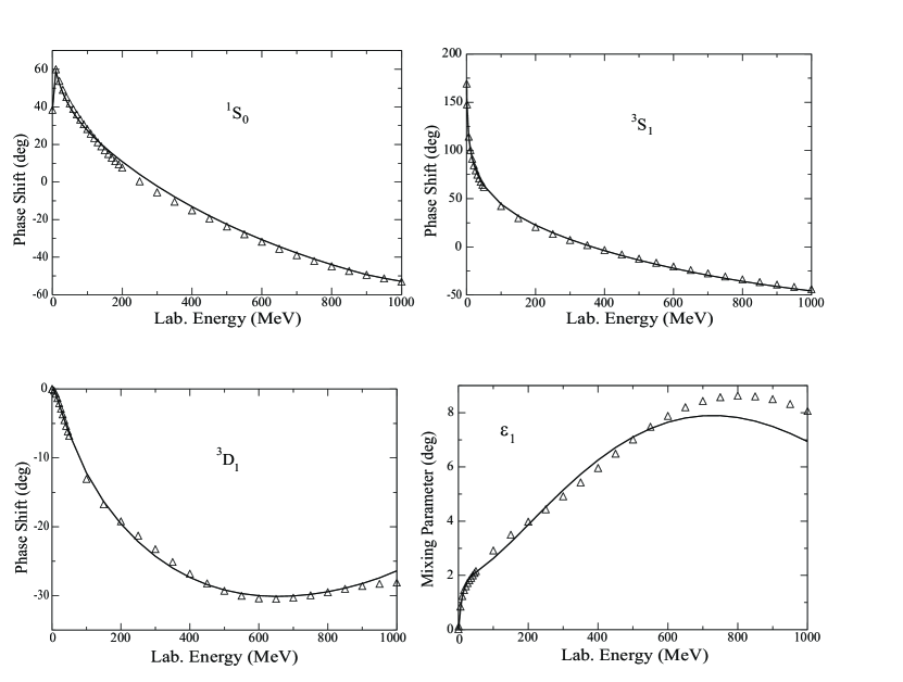
Figure 10: The comparison between the theoretical fits (with the $NN$ potential model similar to that given in eq. (80)) for some lower $NN$ phase shifts and respective phase shift analysis (taken from SAID).

$$V_{NqN}({\bf q},{\bf q}^{\prime})=\lambda^{(0)}f_{00}({\bf q})f_{00}({\bf q}^{\prime})+\widehat{V}_{NqN}^{(2\rm{s})}({\bf q},{\bf q}^{\prime},E),$$ (92)

where the matrix operator $\widehat{V}_{NqN}^{(2\rm{s})}$ takes the form:

$$\widehat{V}_{NqN}^{(2\rm{s})}=\left(\begin{array}[]{cc}\lambda_{(00)}^{(2)}(E)f_{0}({\bf q})f_{0}({\bf q}^{\prime})&\lambda_{(02)}^{(2)}(E)f_{0}({\bf q})f_{2}({\bf q}^{\prime})\\ \lambda_{(20)}^{(2)}(E)f_{2}({\bf q})f_{0}({\bf q}^{\prime})&\lambda_{(22)}^{(2)}(E)f_{2}({\bf q})f_{2}({\bf q}^{\prime})\end{array}\right).$$ (93)

One can attain a quite good description of the triplet phase shift in the whole energy range 0–1 GeV even when choosing the one common value of the oscillator radius for the $s$-wave, $f_{0}({\bf q})$, and $d$-wave, $f_{2}({\bf q})$, potential form factors in Eq. (93). The parameter $a$, that determines the energy variation of all the strength parameters $\lambda_{(ij)}^{(2)}$ is kept the same as in ${}^{1}S_{0}$-channel. So that in the ${}^{3}S_{1}$-${}^{3}D_{1}$ coupled channel case, one has (except of two parameters in $V_{\rm{TPE}}$) only three adjustable strength parameters, viz. $\lambda_{(00)}^{(2)},\ \lambda_{(02)}^{(2)}=\lambda_{(20)}^{(2)}$ and $\lambda_{(22)}^{(2)}$ which make it possible to fit with a good quality the phase shifts together with the respective tensor mixing parameter in a very large energy range 15–1000 MeV (see Fig. 10, upper right and two lower panels).

Thus, the illustrative model derived from EFT-approach developed in the work makes it possible, using physically transparent interaction model with a minimal number of free parameters, to fit very reasonably the phase shifts in ${}^{1}S_{0}$ and ${}^{3}S_{1}$-${}^{3}D_{1}$ channels in the large energy range and the deuteron structure as well. This description can be compared to the fit quality for the phase shifts given by a purely phenomenological separable interaction (of conventional type) of Graz group [52]. The latter model includes more than twenty five free parameters to fit the phase shifts in the same channels until 500 MeV only. Thus the description of the elastic $NN$ scattering given by the present illustrative model derived from EFT-formalism looks highly superior the description attained with the phenomenological separable models.

It is worth to emphasize here that, at the value of the string excitation quantum $\Omega\approx 300-350$ MeV, taking up to two-quanta excitations of the string will be sufficient for description of $NN$-interaction from zero energy until 1 GeV or even higher, while account of four-quanta excitations is sufficient for description of interaction in $NN$-channel or the $NN$ meson-production processes up to energies of $E_{\mathrm{lab}}\approx 3$ GeV.

5 Applications to other hadronic processes

5.1 Description of inelastic processes with the effective field theory approach

Having developed the field-theoretical formalism for the description of the $NN$ elastic scattering in the GeV region one can apply this also to describe inelastic processes within the same framework, i.e. with the same input constants etc. And this possibility is one of main advantage of this unified approach. For the sake of brevity we will omit many details here and illustrate the description of inelastic processes by some graphs only.

In the above field-theoretical formalism the inelastic processes are tightly interrelated to the elastic ones above the respective thresholds through the unitarity relation:

$$T-T^{\dagger}=2\mathrm{i}\,\mathrm{Im}TT^{\dagger},$$ (94)

which corresponds in our language to the respective cuts of the diagrams across the meson loops.

So, the respective meson production amplitudes can be illustrated by the graphs shown in Fig. 11. The left graph relates to $2\pi$-production in $pp$-collisions through the intermediate $\sigma$-meson in the dressed bag, while the graph on the right relates to the near-threshold $\omega$-meson production to the intermediate $N^{*}$-isobar generation. It should be stressed here that the $NN$ “distorted waves” in such meson production amplitudes are generated from the same diagrams (with the same parameter values) as these meson productions. So the approach can be made quite consistent and universal both for elastic and inelastic processes.

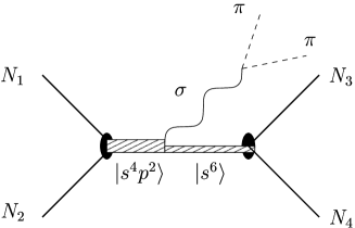
Figure 11: Example of diagrams describing a new possible mechanisms of meson production. Left diagram corresponds to double pion production in the scalar-isoscalar channel, whereas the right one describes an enhancement of the probability for the formation of nucleon excited states and, in particular, of the mechanism of $\omega$-meson emission in a nucleon-nucleon collision.

Another very important issue which can be answered on the basis of the developed approach is multi-meson production and generation of the so called cumulative pions in high-energy $pp$ collisions. According to the relativistic picture presented here, the multi-meson production should correspond to $N\hbar\Omega$ excitation of the intermediate string ($N>>1$) with its subsequent deexcitation by multi-meson emission or by hadronic jets.

By a similar mechanism one can get the emission of cumulative pions (i.e. forbidden in a single-nucleon emission), e.g. in the process $d+\mathrm{A}\rightarrow\pi+\ldots$, where the energy of outgoing pion is larger then half energy of the incident deuterons.

5.2 Treatment of electromagnetic processes at high momentum transfer and new electromagnetic exchange currents

The appearance of the dibaryon component in a nucleus can modify noticeably the nucleon momentum distribution probed at large momentum transfer. E.g. one gets some new contributions to electromagnetically induced two-nucleon knock-out processes in which the emerging two nucleons (from the excited dibaryon decay) escape from the dibaryon state in “back-to-back” kinematics. In fact, just this kinematics was observed for the two-nucleon ejection in many experiments of this type. It is evident that such contributions for the $\mathrm{A}(e,e^{\prime}pp)$ and $\mathrm{A}(\gamma,pp)$ processes at high (virtual) momenta or energies of $\gamma$-quantum must contribute to the reaction cross sections. In such two-nucleon processes, when treated within our approach, the virtual high-energy (or momentum) can be absorbed by the string (i.e. by the dibaryon as a whole) resulting in its excitation followed by either meson emission or break up of the excited dibaryon into the two high-energy nucleons (see e.g. the Fig. 12). Also, the inverse process of bremsstrahlung in $pp$-scattering: $pp\rightarrow pp\gamma$ should be analysed with the same new currents.

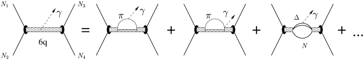
Figure 12: The graphs illustrating the new $3N$ scalar force induced by $\sigma$-exchange between the dressed bag and third nucleon.

Figure 13: Examples of diagrams involving new meson-exchange electromagnetic currents that arise in the present model.

Another good test of the force model developed here will be in prediction of the main characteristic features of e.-m. processes like $\@@nuc{12}{C}(\vec{\gamma},pN)$, $\@@nuc{3}{He}(e,e^{\prime}pN)$, or $\@@nuc{3}{He}(\vec{\gamma},pn)$ with linearly or circularly polarized $\gamma$-quanta which are planned to be measured in Mainz [53]. For calculations of such processes our very accurate $\@@nuc{3}{He}$ wavefunctions [36, 37] found with the above force model can be employed jointly with new e.-m. currents tightly interrelated to the dressed dibaryon degree of freedom. Some diagrams for these new $s$-channel currents in two-nucleon systems are displayed in Fig. 13.

The $s$-channel meson-exchange currents for $(\gamma,pp)$ or $(e,e^{\prime}pp)$ processes should be confronted with the traditional $t$-channel currents for $(pn)$-subsystem (see the Fig. 14) and we can conclude from this comparison that both types of currents, i.e. $t$- and $s$-channel ones can be considered as a complementary to each other. In other words, those $t$-channel currents which disappear in the $pp$-system (i.e. pion-in-flight etc.) will appear in form of $s$-channel currents. The same occurs also for $pn$-system.

Thus the processes like $\@@nuc{3}{He}(e,e^{\prime}pp)$ or $\@@nuc{3}{He}(e,e^{\prime}pn)$ or $\@@nuc{3}{He}(\gamma,pp)$ should be a very good test for the new electromagnetic currents. Hence, the dressed dibaryon component and new currents associated with it should modify the results of the theoretical interpretations of many dedicated experiments done at moderate to high momentum and energy transfers, especially those which are now going on or are planned at Mainz and Bonn.

Figure 14: Example of diagrams for $pn$ bremsstrahlung within traditional OBE-models of the nucleon-nucleon interaction.

5.3 Description of short-range $2N$ and $3N$ correlations in nuclei

The first attempts to apply the DBS-model for description of properties of three-nucleon systems [36, 37] was very successful. In particular, it has been clearly demonstrated that the new short-range three-body attractive force induced by $\sigma$-meson exchange between the DBS and third nucleon (see the Fig. 13) with the $g_{\sigma NN}$ coupling constant adjusted to give the $\@@nuc{3}{H}$ binding energy gives an important contribution to the $3N$ binding energy and other properties of $3N$-system, and can explain quantitatively all static properties of $\@@nuc{3}{He}$ and $\@@nuc{3}{H}$ ground states, including a precise parameter-free description of the Coulomb displacement energy of $\@@nuc{3}{He}$–$\@@nuc{3}{H}$ [37], and all the charge distributions in these nuclei.

In these $3N$ calculations done within the above dibaryon $NN$-force model with additional incorporation of three-nucleon scalar forces shown by the graphs in the Fig. 13, the weight of the dibaryon component in the $3N$ wave function reaches as much as $10-11$% and its contribution to the total $3N$ binding energy is about 50% (!). In other words, half of the total nuclear binding comes from the strong interaction of dibaryon with surrounding nucleons via the $\sigma$-meson exchange [36]. Another important conclusion of these $3N$ calculations is a strong density dependence of the effective two- and three-body forces induced by the intermediate dibaryon generation. The density dependence has a repulsive character and is qualitatively similar to that assumed in the phenomenological Skyrme model. It is very likely that just the interplay between the above density dependent repulsion and $2N$ and $3N$ attraction related to the scalar meson exchange provides the saturation property of nuclear matter.

6 Conclusions

We developed in the work some covariant effective field-theoretical approach toward the description of intermediate- and short-range components of $NN$ interaction and nuclear forces. The approach assumes that the nucleon-nucleon interaction at intermediate and short ranges has a very complicated and multistep character. In the first step, the two-nucleon system goes, by color exchange, to the confined two-cluster $CC$ configuration where the quark clusters are moving at the end of a quantum string (inside of which the gluon fields are localized). Excitations (i.e. vibrations and rotations) of this string can be described by a relativistic covariant harmonic oscillator with a linear confinement potential which leads quite naturally to the linear Regge-trajectory of the respective excited levels of the string. In the next step, the string interacts with vacuum meson fields (mainly $\pi,\sigma$ and $\omega$) and thus it goes to the dibaryon stage by the respective dressing. It is shown that $2\hbar\Omega$-excitation of the string generates a strong scalar $\sigma$-field which, due to the strong attraction to the six-quark core, will compress and stabilize the resulting dressed six-quark bag.

In some aspect the emerged picture should be rather similar to the concept of “small chiral bag” suggested long ago by Brown and Rho [54]. In their model the $3q$-MIT bag is compressed by the strong pressure of its pion (chiral) field to the small size where the additional inner kinetic pressure of free quarks will compensate the external pressure of the pion field to the bag surface. In our case, in contrast to the above “small bag model”, the main meson field is a strong scalar $\sigma$-field which interacts with the six quark system in the whole volume of the bag rather than on the its surface only. Another great difference from the Brown-Rho model is the origin of the stabilizing field ($\sigma$ in our case). In our approach the main component of this scalar field is emerged in deexcitation of the string from $2\hbar\Omega$ to $0\hbar\Omega$ states. Thus, in this process one observes the transformation of the “color” energy of gluon fields (inside the string) to the “white” energy of scalar meson field.

In the next stage of the process, the $\sigma$ field will compress and stabilize the six-quark bag and shift strongly its mass down to the pion-production threshold. Thus this shift should be included to the polarization operator $\Pi(P^{2})$ of the total string propagator. Further, keeping in mind a strong coupling of the $\sigma$-meson to the two-pion channel one can predict from this specific dressing mechanism an enhanced two-pion production in $NN$ collision as compared to the traditional OBE-models, the feature just observed experimentally. Moreover, almost the same mechanism can enhance quite naturally the single-pion production in $pp$-collision and especially the near threshold $\pi_{0}$ production. The consistent theoretical explanation of which met so serious problems in the recent decade [22]. Moreover, a quite similar two-stage mechanism (in first stage, the excitation of the color string with the subsequent transformation of the “color” string energy to the meson fields) should be responsible for multi-meson production in $NN$ and heavy ion collisions. So, by this way, the multi-meson production in high-energy heavy-ion collision may give a good test for the proposed color string model. The authors plan to return to this point in their next papers.

References

- [1] A.D. Lahiff, I.R. Afnan, Phys. Rev. C 60 (1999) 024608.
- [2] A. Nogga, H. Kamada, W. Glöckle, Phys. Rev. Lett. 85 (2000) 944.
- [3] V.I. Kukulin, I.T. Obukhovsky, V.N. Pomerantsev, A. Faessler, Phys. At. Nucl. 64 (2001) 1667.
- [4] D. Plaemper, J. Flender, M.F. Gari, Phys. Rev. C 49 (1994) 2370.
- [5] T. Sasakawa, S. Ishikawa, Few Body Syst. 1 (1986) 3.
- [6] R.S. Hicks et al., Phys. Rev. C 67 (2003) 064004; F. Moschini, Proc. of 6th Workshop on “e-m induced Two-Hadron Emission”, Pavia, September 24-27, 2003, p. 156.
- [7] D.L. Groep et al., Phys. Rev. C 63 (2001) 014005.
- [8] S. Ishikawa, J. Golak, H. Witala, H. Kamada, W. Glöckle, D. Hüber, Phys. Rev. C 57 (1998) 39; R. Skibiński et al., Phys. Rev. C 67 (2003) 054002; W. Glöckle et al., Proc. of 6th Workshop on “e-m induced Two-Hadron Emission”, Pavia, September 24-27, 2003, p. 166.
- [9] E. Jans, P. Barneo, Proc. of 6th Workshop on “e-m induced Two-Hadron Emission”, Pavia, September 24-27, 2003, p. 183.
- [10] L.B. Weinstein, Proc. of 5th Workshop on “e-m induced Two-Hadron Emission”, Lund, June 13-16, 2001, p. 93; E. Piasetzky, R. Gilman, M. Sargsian, Proc. of 6th Workshop on “e-m induced Two-Hadron Emission”, Pavia, September 24-27, 2003, p. 211.
- [11] J.-M. Laget, Nucl. Phys. A 579 (1994) 333.
- [12] F. Stancu, Few Body Syst. Suppl. 14 (2003) 83; D. Bartz, F. Stancu, Phys. Rev. C 63 (2001) 034001; Nucl. Phys. A 699 (2002) 316.
- [13] R.V. Mau, Prog. Part. Nucl. Phys. 50 (2003) 561.
- [14] M. Oka, K. Shimizu, K. Yazaki, Prog. Theor. Phys. Suppl. 137 (2000) 1.
- [15] D.R. Entem, F. Fernández, A. Valcarce, Phys. Rev. C 62 (2000) 034002; C 67 (2003) 014001.
- [16] S. Weinberg, Phys. Lett. B 251 (1990) 288; Nucl. Phys. B 363 (1991) 3.
- [17] D.B. Kaplan, nucl-th/9506035; Nucl. Phys. B 494 (1997) 471; D.B. Kaplan, M. Savage, M.B. Wise, Nucl. Phys. B 478 (1996) 629; Phys. Lett. B 424 (1998) 390.
- [18] D.R. Entem, R. Machleidt, Phys. Rev. C 68 (2003) 041001.
- [19] E. Epelbaum, W. Glöckle, U.G. Meissner, Eur. Phys. J. A 19 (2004) 125.
- [20] R. Higa, M.R. Robilotta, Phys. Rev. C 68 (2003) 024004; R. Higa, M.R. Robilotta, C.A. da Rocha, Phys. Rev. C 69 (2004) 034009.
- [21] H.O. Meyer et al., Phys. Rev. C 63 (2001) 064002.
- [22] C. Hanhart, Phys. Rep. 397 (2004) 155.
- [23] B. von Przewoski et al., Phys. Rev. C 58 (1998) 1897.
- [24] W.W. Daehnick et al., Phys. Rev. C 65 (2002) 024003.
- [25] Bo Höistad, Nucl. Phys. A 721, (2003) 570c; J. Johanson et al., Nucl. Phys. A 712 (2002) 75.
- [26] F. Shimizu et. al., Nucl. Phys. A 386 (1982) 571.
- [27] L. Alvarez-Ruso, E. Oset, E. Hernandez, Nucl. Phys. A 633 (1998) 519.
- [28] S.J. Brodsky, L. Frankfurt, R. Gilman, J.R. Hiller, G.A. Miller, E. Piasetzky, M. Sargsian, M. Strikman, Phys. Lett. B 578 (2004) 69.
- [29] V.I. Kukulin, V.N. Pomerantsev, A. Faessler, J. Phys. G 27 (2001) 1851.
- [30] V.I. Kukulin, I.T. Obukhovsky, V.N. Pomerantsev, A. Faessler, Int. J. Mod. Phys. E 11 (2002) 1.
- [31] E.M. Nyman, D.O. Riska, Phys. Scripta 34 (1986) 533; Phys. Lett. B 203 (1988) 13.
- [32] E. Oset, H. Toki, M. Mizobe, T.T. Takahashi, Progr. Theor. Phys. 103 (2000) 351.
- [33] M.M. Kaskulov, H. Clement, Phys. Rev. C 70 (2004) 014002.
- [34] N. Kaiser, U.G. Meissner, Phys. Lett. B 233 (1989) 457.
- [35] V.I. Kukulin, Few Body Syst. Suppl. 14 (2003) 71.
- [36] V.I. Kukulin, V.N. Pomerantsev, M.M. Kaskulov, A. Faessler, J. Phys. G 30 (2004) 287.
- [37] V.I. Kukulin, V.N. Pomerantsev, A. Faessler, J. Phys. G 30 (2004) 309.
- [38] I.T. Obukhovsky, V.I. Kukulin, M.M. Kaskulov, P. Grabmayr, A. Faessler, J. Phys. G 29 (2003) 2207.
- [39] V.I. Kukulin, M.A. Shikhalev, Phys. At. Nucl. 67 (2004) 1536.
- [40] M.M. Kaskulov, P. Grabmayr, V.I. Kukulin, Int. J. Mod. Phys. E 12 (2003) 449; M.M. Kaskulov, V.I. Kukulin, P. Grabmayr, Few Body Syst. Suppl. 14 (2003) 101.
- [41] A.M. Kusainov, V.G. Neudatchin, I.T. Obukhovsky, Phys. Rev. C 44 (1991) 2343.
- [42] P. Faccioli, E.V. Shuryak, Phys. Rev. D 65 (2002) 076002.
- [43] R. Rapp, T. Schafer, E. Shuryak, M. Velkovsky, Phys. Rev. Lett. 81 (1998) 53.
- [44] M. Alford, K. Rajagopal, F. Wilczek, Phys. Lett. B 422 (1998) 247.
- [45] M. Huang, P.F. Zhuang, W.Q. Chao, Phys. Rev. D 65 (2002) 076012.
- [46] F. Wilczek, hep-ph/0409168.
- [47] D. Bartz, Fl. Stancu, Phys. Rev. C 59 (1999) 1756.
- [48] J.D. Björken, S.D. Drell, Relativistic Quantum Mechanics, McGraw–Hill, New York, 1964.
- [49] R.P. Feynman, M. Kislinger, F. Ravndal, Phys. Rev. D 3 (1971) 2706; S. Ishida, M. Ishida, T. Maeda, Prog. Theor. Phys. 104 (2000) 785.
- [50] M. Moshinsky, A. Szczepaniak, J. Phys. A 22 (1989) L817; A. Szczepaniak, A.G. Williams, Phys. Rev. D 47 (1993) 1175.
- [51] T. Takabayasi, Phys. Rev. B 139 (1965) B1381; Suppl. Prog. Theor. Phys. 67 (1979) 1.
- [52] L. Mathelitsch, W. Plessas, M. Schweiger, Phys. Rev. C 26 (1982) 65.
- [53] C.J.Y. Powrie et al., Phys. Rev. C 64 (2001) 034602.
- [54] G.E. Brown, M. Rho, Comments Nucl. Part. Phys. 18 (1988) 1; see also S.W. Hong and B.K. Jennings, Phys. Rev. C 64 (2001) 038203.