An analytic collective model in which the relative presence of the quadrupole and octupole deformations is determined by a parameter ($\phi_{0}$), while axial symmetry is obeyed, is developed. The model [to be called the analytic quadrupole octupole axially symmetric model (AQOA)] involves an infinite well potential, provides predictions for energy and $B(EL)$ ratios which depend only on $\phi_{0}$, draws the border between the regions of octupole deformation and octupole vibrations in an essentially parameter-independent way, and describes well ²²⁶Th and ²²⁶Ra, for which experimental energy data are shown to suggest that they lie close to this border. The similarity of the AQOA results with $\phi_{0}=45^{\rm o}$ for ground state band spectra and $B(E2)$ transition rates to the predictions of the X(5) model is pointed out. Analytic solutions are also obtained for Davidson potentials of the form $\beta^{2}+\beta_{0}^{4}/\beta^{2}$, leading to the AQOA spectrum through a variational procedure.

PACS numbers: 21.60.Ev, 21.60.Fw, 21.10.Re

Section: Nuclear Structure

1. Introduction

Rotational nuclear spectra have long been attributed to quadrupole deformations [1], while octupole deformations [corresponding to reflection asymmetric (pearlike) shapes] are supposed to occur in certain regions, most notably in the light actinides [2, 3, 4, 5]. The hallmark of octupole deformation is a negative parity band with levels $L^{\pi}=1^{-}$, $3^{-}$, $5^{-}$, …, lying close to the ground state band and forming with it a single band with $L^{\pi}=0^{+}$, $1^{-}$, $2^{+}$, $3^{-}$, $4^{+}$, …, while a negative parity band lying systematically higher than the ground state band is a footprint of octupole vibrations. The transition from the regime of octupole vibrations into the region of octupole deformation has been considered by several authors [6, 7, 8]. A complete algebraic classification of the states occuring in the simultaneous presence of the quadrupole and octupole degrees of freedom has been provided in terms of the spdf-interacting boson model [9, 10], involving free parameters. (It should be noted, however, that an alternative interpretation of the low-lying negative parity states in the light actinides has been provided in terms of clustering [11, 12, 13].)

On the other hand, the transitions from vibrational [U(5)] shapes to axially symmetric deformed [SU(3)] and $\gamma$-unstable deformed [SO(6)] shapes have been recently described in terms of the X(5) [14] and E(5) [15] models respectively, which utilize an infinite well potential in the $\beta$ degree of freedom, leading to parameter-free (up to overall scale factors) predictions for spectra and transition probabilities.

It is the aim of the present work to provide an analytic description of the light actinides lying near the border between the regions of octupole vibrations and octupole deformation, through the use of a model containing the minimum number of free parameters. In this direction, the following steps are taken:

1) Quadrupole and octupole deformations are taken into account on equal footing, their relative presence decided by the only free parameter in the model, $\phi_{0}$.

2) Axial symmetry is assumed, in order to keep the problem tractable.

3) Symmetrization of the wave functions is carried out as in Ref. [16], involving the irreducible representation (irrep) A of the group D₂ for the levels of even parity and the irrep B₁ of the same group for the levels of odd parity.

4) Separation of variables is achieved in a way analogous to the one used in the framework of the X(5) model [14].

5) An infinite well potential is assumed appropriate for the description of the border region, as in the E(5) [15] and X(5) [14] models.

The predictions of the model, to be called AQOA, are compared to spectra and $B(EL)$ ratios for ²²⁶Th and ²²⁶Ra, for which evidence from systematics of experimental data is presented, suggesting that they lie close to the border between octupole deformation and octupole vibrations. This border is found to be drawn by the AQOA model in an essentially parameter-independent way.

In addition, solutions for Davidson potentials [17] of the form $\beta^{2}+\beta_{0}^{4}/\beta^{2}$ are obtained, and a variational method [18, 19] leading from the Davidson results to the AQOA predictions is worked out.

A different approach to the problem of phase transition in the octupole mode has been recently given in Ref. [20], where the starting point is the introduction of a new parametrization of the quadrupole and octupole degrees of freedom, using as intrinsic frame of reference the principal axes of the overall tensor of inertia, as resulting from the combined quadrupole and octupole deformation. Comparisons between the results of the two methods are deferred to the appropriate sections. Three main differences between the two models are:

1) The AQOA model is analytic, while the model of Ref. [20] is not.

2) In the AQOA model the quadrupole and octupole degrees of freedom are taken into account on equal footing, while in the special form of the model of Ref. [20] used for comparison to experiment, the octupole degree of freedom remains active, while the quadrupole degree of freedom is “frozen” to a constant value.

3) In the AQOA model the symmetry axes of the quadrupole and octupole deformations are taken to coincide, in order to guarantee axial symmetry, while in the more general framework of Ref. [20] nonaxial contributions, small but not frozen to zero, are taken into account.

In Section 2 the AQOA model is formulated, while numerical results are given in Section 3 and compared to experiment in Section 4. In Section 5 the variational procedure is described, while Section 6 contains discussion of the present results and plans for further work.

2. The Analytic Quadrupole Octupole Axially Symmetric (AQOA) Model

2.1 Formulation

We consider a nucleus in which quadrupole deformation ($\beta_{2}$) and octupole deformation ($\beta_{3}$) coexist. We take only axially symmetric deformations into account, which implies that the $\gamma$ degrees of freedom are ignored, as in the Davydov–Chaban approach [21]. The body-fixed axes $x^{\prime}$, $y^{\prime}$, $z^{\prime}$ are taken along the principal axes of inertia of the (axially symmetric) nucleus, while their orientation relative to the laboratory-fixed axes $x$, $y$, $z$ is described by the Euler angles $\theta=\{\theta_{1},\theta_{2},\theta_{3}\}$. The Hamiltonian reads [16, 22]

$$H=-\sum_{\lambda=2,3}{\hbar^{2}\over 2B_{\lambda}}{1\over\beta_{\lambda}^{3}}{\partial\over\partial\beta_{\lambda}}\beta_{\lambda}^{3}{\partial\over\partial\beta_{\lambda}}+{\hbar^{2}\hat{L^{2}}\over 6(B_{2}\beta_{2}^{2}+2B_{3}\beta_{3}^{2})}+V(\beta_{2},\beta_{3})$$ (1)

where $B_{2}$, $B_{3}$ are the mass parameters.

We seek solutions of the Schrödinger equation of the form [16]

$$\Phi^{\pm}_{L}(\beta_{2},\beta_{3},\theta)=(\beta_{2}\beta_{3})^{-3/2}\Psi^{\pm}_{L}(\beta_{2},\beta_{3})|LM0,\pm\rangle,$$ (2)

where the function $|LM0,\pm\rangle$ describes the rotation of an axially symmetric nucleus with angular momentum projection $M$ onto the laboratory-fixed $z$-axis and projection $K=0$ onto the body-fixed $z^{\prime}$-axis. The moment of inertia with respect to the symmetry axis $z^{\prime}$ is zero, implying that levels with $K\neq 0$ lie infinitely high in energy [16]. Therefore in this model we are restricted to states with $K=0$ only. The function $|LM0,+\rangle$ transforms according to the irreducible representation (irrep) A of the group D₂, while the function $|LM0,-\rangle$ transforms according to the irrep B₁ of the same group [16, 22]. The general form of these functions is [1]

$$|LMK,\pm\rangle=\sqrt{2L+1\over 16\pi^{2}(1+\delta_{K0})}({\cal D}^{L}_{K,M}(\theta)\pm(-1)^{L}{\cal D}^{L}_{-K,M}(\theta)).$$ (3)

In the special case of $K=0$ it is clear that $|LM0,+\rangle\neq 0$ for $L=0$, 2, 4, …, while $|LM0,-\rangle\neq 0$ for $L=1$, 3, 5, …The functions $\Psi_{L}^{+}(\beta_{2},\beta_{3})$ and $\Psi_{L}^{-}(\beta_{2},\beta_{3})$ are respectively symmetric and antisymmetric with respect to reflection in the plane $x^{\prime}y^{\prime}$, and therefore describe states with positive and negative parity respectively [22].

Using the solutions of Eq. (2) for the Hamiltonian of Eq. (1) the Schrödinger equation takes the simplified form

$$\left[-{\hbar^{2}\over 2B_{2}}{\partial^{2}\over\partial\beta_{2}^{2}}-{\hbar^{2}\over 2B_{3}}{\partial^{2}\over\partial\beta_{3}^{2}}+{\hbar^{2}L(L+1)\over 6(B_{2}\beta_{2}^{2}+2B_{3}\beta_{3}^{2})}\right.$$

$$\left.+V(\beta_{2},\beta_{3})+{3\hbar^{2}\over 8}\left({1\over B_{2}\beta_{2}^{2}}+{1\over B_{3}\beta_{3}^{2}}\right)-E_{L}\right]\Psi^{\pm}_{L}(\beta_{2},\beta_{3})=0.$$ (4)

This equation is further simplified by introducing [16, 22]

$$\tilde{\beta}_{2}=\beta_{2}\sqrt{B_{2}\over B},\quad\tilde{\beta}_{3}=\beta_{3}\sqrt{B_{3}\over B},\quad B={B_{2}+B_{3}\over 2},$$ (5)

as well as reduced energies $\epsilon=(2B/\hbar^{2})E$ and reduced potentials $u=(2B/\hbar^{2})V$ [14, 15], reaching the form

$$\left[-{\partial^{2}\over\partial\tilde{\beta}_{2}^{2}}-{\partial^{2}\over\partial\tilde{\beta}_{3}^{2}}+{L(L+1)\over 3(\tilde{\beta}_{2}^{2}+2\tilde{\beta}_{3}^{2})}+u(\tilde{\beta}_{2},\tilde{\beta}_{3})+{3\over 4}\left({1\over\tilde{\beta}_{2}^{2}}+{1\over\tilde{\beta}_{3}^{2}}\right)-\epsilon_{L}\right]\Psi_{L}^{\pm}(\tilde{\beta}_{2},\tilde{\beta}_{3})=0.$$ (6)

Further simplification occurs through the introduction of polar coordinates (with $0\leq\tilde{\beta}<\infty$ and $-\pi/2\leq\phi\leq\pi/2$) [16, 22]

$$\tilde{\beta}_{2}=\tilde{\beta}\cos\phi,\quad\tilde{\beta}_{3}=\tilde{\beta}\sin\phi,\quad\tilde{\beta}=\sqrt{\tilde{\beta}_{2}^{2}+\tilde{\beta}_{3}^{2}},$$ (7)

leading to

$$\left[-{\partial^{2}\over\partial\tilde{\beta}^{2}}-{1\over\tilde{\beta}}{\partial\over\partial\tilde{\beta}}+{L(L+1)\over 3\tilde{\beta}^{2}(1+\sin^{2}\phi)}-{1\over\tilde{\beta}^{2}}{\partial^{2}\over\partial\phi^{2}}+u(\tilde{\beta},\phi)+{3\over\tilde{\beta}^{2}\sin^{2}2\phi}-\epsilon_{L}\right]\Psi_{L}^{\pm}(\tilde{\beta},\phi)=0.$$ (8)

It is clear that $\phi=0$ corresponds to quadrupole deformation alone, while $\phi=\pm\pi/2$ corresponds to octupole deformation alone. It is worth noticing that the transformation of Eq. (7) allows $\beta_{3}$ to assume both positive and negative values, while $\beta_{2}$ takes only positive values.

Separation of variables in Eq. (8) can be achieved by assuming the potential to be of the form $u(\tilde{\beta},\phi)=u(\tilde{\beta})+u(\tilde{\phi}^{\pm})$, where $u(\tilde{\phi}^{\pm})$ is supposed to be of the form of two very steep harmonic oscillators centered at the values $\pm\phi_{0}$, i.e.

$$u(\tilde{\phi}^{\pm})={1\over 2}c(\phi\mp\phi_{0})^{2}={1\over 2}c(\tilde{\phi}^{\pm})^{2},\qquad\tilde{\phi}^{\pm}=\phi\mp\phi_{0},$$ (9)

with $c$ being a large constant. In other words, the nucleus is supposed to be rigid with respect to the variable $\phi$, implying that $\phi$ remains close to $\pm\phi_{0}$ and, therefore, the relative amount of quadrupole and octupole deformation remains constant, as in Strutinsky-type potential energy calculations [6]. This assumption will be (partly) justified a posteriori by the fact that the spectrum remains almost unchanged for values of $\phi_{0}$ between 30^o and 60^o.

In this way Eq. (8) is separated into

$$\left[-{\partial^{2}\over\partial\tilde{\beta}^{2}}-{1\over\tilde{\beta}}{\partial\over\partial\tilde{\beta}}+{1\over\tilde{\beta}^{2}}\left({L(L+1)\over 3(1+\sin^{2}\phi_{0})}+{3\over\sin^{2}2\phi_{0}}\right)+u(\tilde{\beta})-\epsilon_{\tilde{\beta}}(L)\right]\psi_{L}^{\pm}(\tilde{\beta})=0,$$ (10)

and

$$\left[-{1\over\langle\tilde{\beta}^{2}\rangle}{\partial^{2}\over\partial(\tilde{\phi}^{\pm})^{2}}+u(\tilde{\phi}^{\pm})-\epsilon_{\phi}\right]\chi(\tilde{\phi}^{\pm})=0,$$ (11)

where $\Psi_{L}^{\pm}(\tilde{\beta},\phi)=\psi_{L}^{\pm}(\tilde{\beta})(\chi(\tilde{\phi}^{+})\pm\chi(\tilde{\phi}^{-}))/\sqrt{2}$, while $\langle\tilde{\beta}^{2}\rangle$ is the average of $\tilde{\beta}^{2}$ over $\psi^{\pm}(\tilde{\beta})$, and $\epsilon_{L}=\epsilon_{\tilde{\beta}}(L)+\epsilon_{\phi}$. It is worth noticing that Eq. (10) has the same form for both $+\phi_{0}$ and $-\phi_{0}$, since only even functions of $\phi_{0}$ appear in it.

2.2 The $\tilde{\beta}$-part of the spectrum

In the case in which $u(\tilde{\beta})$ is an infinite well potential ($u(\tilde{\beta})=0$ if $\tilde{\beta}\leq\tilde{\beta}_{W}$; $u(\tilde{\beta})=\infty$ if $\tilde{\beta}>\tilde{\beta}_{W}$), using the definitions $\epsilon_{\tilde{\beta}}=k_{\tilde{\beta}}^{2}$, $z=\tilde{\beta}k_{\tilde{\beta}}$, Eq. (10) is brought into the form of a Bessel equation

$${d^{2}\psi_{\nu}^{\pm}\over dz^{2}}+{1\over z}{d\psi_{\nu}^{\pm}\over dz}+\left[1-{\nu^{2}\over z^{2}}\right]\psi_{\nu}^{\pm}=0,$$ (12)

with

$$\nu=\sqrt{{L(L+1)\over 3(1+\sin^{2}\phi_{0})}+{3\over\sin^{2}2\phi_{0}}}.$$ (13)

Then the boundary condition $\psi_{\nu}^{\pm}(\tilde{\beta}_{W})=0$ determines the spectrum

$$\epsilon_{\tilde{\beta},s,\nu}=\epsilon_{\tilde{\beta},s,\phi_{0},L}=(k_{s,\nu})^{2},\qquad k_{s,\nu}={x_{s,\nu}\over\tilde{\beta}_{W}},$$ (14)

and the eigenfunctions

$$\psi_{s,\nu}^{\pm}(\tilde{\beta})=\psi^{\pm}_{s,\phi_{0},L}(\tilde{\beta})=c_{s,\nu}J_{\nu}(k_{s,\nu}\tilde{\beta}),$$ (15)

where $x_{s,\nu}$ is the $s$th zero of the Bessel function $J_{\nu}(z)$, while $c_{s,\nu}$ are normalization constants, determined from the condition $\int_{0}^{\tilde{\beta}_{W}}|\psi^{\pm}_{s,\nu}(\tilde{\beta})|^{2}\tilde{\beta}d\tilde{\beta}=1$ to be $c_{s,\nu}=\sqrt{2}/J_{\nu+1}(k_{s,\nu})$. The notation has been kept similar to Ref. [14].

Eq. (10) is also exactly soluble [23, 24] in the case of the Davidson potentials [17]

$$u(\tilde{\beta})=\tilde{\beta}^{2}+{\tilde{\beta}_{0}^{4}\over\tilde{\beta}^{2}}.$$ (16)

In this case the second term of Eq. (16) is combined with the third term of Eq. (10), leading to eigenfunctions which are Laguerre polynomials

$$F^{L}_{n}(\tilde{\beta})=\sqrt{2n!\over\Gamma(n+a+1)}\tilde{\beta}^{a}L_{n}^{a}(\tilde{\beta}^{2})e^{-\tilde{\beta}^{2}/2},$$ (17)

where

$$a=\sqrt{{L(L+1)\over 3(1+\sin^{2}\phi_{0})}+{3\over\sin^{2}2\phi_{0}}+\beta_{0}^{4}}$$ (18)

while the energy eigenvalues are given by

$$E_{n,L}=2n+a+1=2n+1+\sqrt{{L(L+1)\over 3(1+\sin^{2}\phi_{0})}+{3\over\sin^{2}2\phi_{0}}+\beta_{0}^{4}}.$$ (19)

It is worth remarking that the excitation energies, $E_{0,L}-E_{0,0}$, within the ground state band (which is characterized by $n=0$), divided by an appropriate normalization constant read

$$E^{\prime}_{0,L,exc}=\sqrt{1+b_{H}L(L+1)}-1,$$ (20)

with $b_{H}^{-1}=3(1+\sin^{2}\phi_{0})\left({3\over\sin^{2}2\phi_{0}}+\beta_{0}^{4}\right)$. Eq. (20) is the Holmberg–Lipas formula [25].

In what follows, the infinite well potential will be used everywhere. Davidson potentials will be briefly employed in Section 5.

2.3 The $\phi$-part of the spectrum

Eq. (11) for the potential of Eq. (9) takes the form

$$\left[-{\partial^{2}\over\partial(\tilde{\phi}^{\pm})^{2}}+{1\over 2}c\langle\tilde{\beta}^{2}\rangle(\tilde{\phi}^{\pm})^{2}\right]\chi(\tilde{\phi}^{\pm})=\epsilon_{\phi}\langle\tilde{\beta}^{2}\rangle\chi(\tilde{\phi}^{\pm}),$$ (21)

where $\tilde{\phi}^{\pm}=\phi\mp\phi_{0}$. This is a simple harmonic oscillator equation with energy eigenvalues

$$\epsilon_{\phi}=\sqrt{2c\over\langle\tilde{\beta}^{2}\rangle}\left(n_{\phi}+{1\over 2}\right),\qquad n_{\phi}=0,1,2,\ldots$$ (22)

and eigenfunctions

$$\chi_{n_{\phi}}(\tilde{\phi}^{\pm})=N_{n_{\phi}}H_{n_{\phi}}(b\tilde{\phi}^{\pm})e^{-b^{2}(\tilde{\phi}^{\pm})^{2}/2},\qquad b=\left(c\langle\tilde{\beta}^{2}\rangle\over 2\right)^{1/4},$$ (23)

with normalization constant $N_{n_{\phi}}=\sqrt{b\over\sqrt{\pi}2^{n_{\phi}}n_{\phi}!}$.

The total energy in the present model is then

$$E(s,L,\phi_{0},n_{\phi})=E_{0}+A\epsilon_{\tilde{\beta},s,\phi_{0},L}+Bn_{\phi}.$$ (24)

2.4 $B(EL)$ transition rates

In the axial case used here the electric quadrupole and octupole operators are

$$T^{(E2)}_{\mu}=t_{2}\beta_{2}{\cal D}^{(2)}_{\mu,0}(\theta),\qquad T^{(E3)}_{\mu}=t_{3}\beta_{3}{\cal D}^{(3)}_{\mu,0}(\theta),$$ (25)

while the electric dipole operator reads [16]

$$T^{(E1)}_{\mu}=t_{1}\beta_{2}\beta_{3}{\cal D}^{(1)}_{\mu,0}(\theta).$$ (26)

The total wave function in the case of the infinite well potential is

$$\Phi^{\pm}_{L}(\beta_{2},\beta_{3},\theta)=C(\beta_{2}\beta_{3})^{-3/2}J_{\nu}(k_{s,\nu}\tilde{\beta}){(\chi_{n_{\phi}}(\tilde{\phi}^{+})\pm\chi_{n_{\phi}}(\tilde{\phi}^{-}))\over\sqrt{2}}\sqrt{2L+1\over 32\pi^{2}}(1\pm(-1)^{L}){\cal D}^{L}_{0,M}(\theta),$$ (27)

where $C$ is a constant, while in the case of the Davidson potentials the same expression holds with $J_{\nu}(k_{s,\nu}\tilde{\beta})$ replaced by $F^{L}_{n}(\tilde{\beta})$.

$B(EL)$ transition rates are given by

$$B(EL;L_{i}a_{i}\to L_{f}a_{f})={|\langle L_{f}a_{f}||T^{(EL)}||L_{i}a_{i}\rangle|^{2}\over(2L_{i}+1)},$$ (28)

where the reduced matrix element is obtained through the Wigner-Eckart theorem

$$\langle L_{f}\mu_{f}a_{f}|T^{(EL)}_{\mu}|L_{i}\mu_{i}a_{i}\rangle={(L_{i}LL_{f}|\mu_{i}\mu\mu_{f})\over\sqrt{2L_{f}+1}}\langle L_{f}a_{f}||T^{EL}||L_{i}a_{i}\rangle.$$ (29)

In Eq. (28) the integration over the angles $\theta$ involves a standard integral over three Wigner functions [26], which leads to $(L_{i}LL_{f}|000)$, while the rest of the integrations are performed over $\int\int\beta_{2}^{3}d\beta_{2}\beta_{3}^{3}d\beta_{3}$, where the $\beta_{2}^{3}$, $\beta_{3}^{3}$ factors come from the volume element and cancel with the first factor of Eq. (27). Using Eqs. (5) and (7), as well as the relevant Jacobian, one finds (up to constant factors) that the integration is over $\int\tilde{\beta}d\tilde{\beta}d\phi$.

In the integrals over $\phi$, only the case of $n_{\phi}=0$, corresponding to $H_{0}=1$, is considered. The results are factors depending on the parameters $b$ and $\phi_{0}$, as well as on the multipolarity of the transition. Therefore in Section 3, ratios of $B(EL)$ transition rates will be presented, in which these factors cancel out.

The integrals over $\tilde{\beta}$ are

$$I_{\tilde{\beta}}^{(E2)}=I_{\tilde{\beta}}^{(E3)}=\int\tilde{\beta}^{2}J_{\nu_{i}}(k_{s_{i},\nu_{i}}\tilde{\beta})J_{\nu_{f}}(k_{s_{f},\nu_{f}}\tilde{\beta})d\tilde{\beta},$$ (30)

$$I_{\tilde{\beta}}^{(E1)}=\int\tilde{\beta}^{3}J_{\nu_{i}}(k_{s_{i},\nu_{i}}\tilde{\beta})J_{\nu_{f}}(k_{s_{f},\nu_{f}}\tilde{\beta})d\tilde{\beta},$$ (31)

in the case of the infinite well potential, while for the Davidson potentials the Bessel functions are replaced by Laguerre polynomials, as above. The final result then reads

$$B(EL;L_{i}\to L_{f})=c(c_{s_{i},\nu_{i}}c_{s_{f},\nu_{f}})^{2}(L_{i}LL_{f}|000)^{2}(I_{\tilde{\beta}}^{(EL)})^{2},$$ (32)

where $L=1,2,3$ and all constant factors have been absorbed in $c$.

3. Numerical results

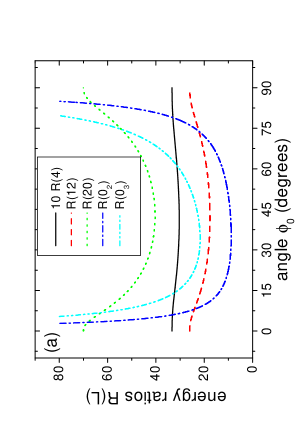
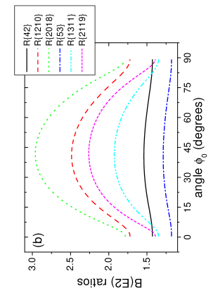
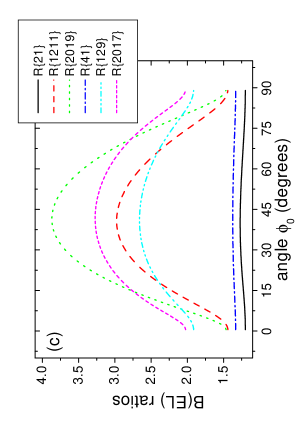
Figure 1: (color online) (a) Energy ratios $R(L)={E(L)\over E(2_{1}^{+})}$ as a function of the angle $\phi_{0}$. The minima appear as follows: $R(4)$ at $41.19^{\rm o}$, $R(12)$ at $42.03^{\rm o}$, $R(20)$ at $42.61^{\rm o}$, $R(0_{2})$ at $34.99^{\rm o}$, $R(0_{3})$ at $34.13^{\rm o}$. (b) Same for the $B(E2)$ ratios $R\{42\}={B(E2;4^{+}\to 2^{+})\over B(E2;2^{+}\to 0^{+})}$ ($40.5^{\rm o}$), $R\{1210\}={B(E2;12^{+}\to 10^{+})\over B(E2;2^{+}\to 0^{+})}$ ($41.0^{\rm o}$), $R\{2018\}={B(E2;20^{+}\to 18^{+})\over B(E2;2^{+}\to 0^{+})}$ ($42.0^{\rm o}$), $R\{53\}={B(E2;5^{-}\to 3^{-})\over B(E2;3^{-}\to 1^{-})}$ ($40.5^{\rm o}$), $R\{1311\}={B(E2;13^{-}\to 11^{-})\over B(E2;3^{-}\to 1^{-})}$ ($41.5^{\rm o}$), $R\{2119\}={B(E2;21^{-}\to 19^{-})\over B(E2;3^{-}\to 1^{-})}$ ($42.0^{\rm o}$). After each ratio, the position of the maximum (with accuracy $\pm 0.5^{\rm o}$) appears in parentheses. (c) Same for the $B(E1)$ ratios $R\{21\}={B(E1;2^{+}\to 1^{-})\over B(E1;1^{-}\to 0^{+})}$ ($40.0^{\rm o}$), $R\{1211\}={B(E1;12^{+}\to 11^{-})\over B(E1;1^{-}\to 0^{+})}$ ($40.5^{\rm o}$), $R\{2019\}={B(E1;20^{+}\to 19^{-})\over B(E1;1^{-}\to 0^{+})}$ ($41.5^{\rm o}$), and for the $B(E3)$ ratios $R\{41\}={B(E3;4^{+}\to 1^{-})\over B(E3;3^{-}\to 0^{+})}$ ($41.0^{\rm o}$), $R\{129\}={B(E3;12^{+}\to 9^{-})\over B(E3;3^{-}\to 0^{+})}$ ($41.0^{\rm o}$), $R\{2017\}={B(E3;20^{+}\to 17^{-})\over B(E3;3^{-}\to 0^{+})}$ ($41.5^{\rm o}$). Again, each ratio is followed by the position of the maximun (with accuracy $\pm 0.5^{\rm o}$) in parentheses.

Spectra for the ground state band and the negative parity band associated with it ($s=1$), as well as for the first excited band ($s=2$) and the second excited band ($s=3$), normalized to the $2_{1}^{+}$ state of the ground state band, are shown for several values of $\phi_{0}$ in Table 1. A few $R(L)=E(L)/E(2)$ ratios are also depicted as functions of $\phi_{0}$ in Fig. 1(a). It is clear that the results are quite stable in the region $30^{\rm o}\leq\phi_{0}\leq 60^{\rm o}$, while at the limiting cases near $\phi_{0}=0^{\rm o}$ and $90^{\rm o}$ the rigid rotor results are obtained, corresponding to a pure rotational spectrum for the ground state band and the associated negative parity band, while the excited bands are pushed to infinity.

$B(E2)$ transition rates are listed in Table 2 for several values of $\phi_{0}$, while a few $B(E2)$ ratios are shown in Fig. 1(b) as functions of $\phi_{0}$, their behavior being quite smooth in the region $30^{\rm o}\leq\phi_{0}\leq 60^{\rm o}$. The same remark applies to $B(E1)$ and $B(E3)$ transitions, listed in Tables 3 and 4, and shown in Fig. 1(c).

It is worth remarking that the minima of energy ratios related to the ground state band, as well as the maxima of $B(EL)$ ratios regarding the ground state band and the associated negative parity band, reported in the caption of Fig. 1, are all located between $\phi_{0}=40^{\rm o}$ and $43^{\rm o}$, while the minima of energy ratios regarding the excited ($s=2$, 3) bands are located near $\phi_{0}=35^{\rm o}$.

The tables and figures mentioned so far indicate that the region of interest in the present model, in which smooth and essentially parameter independent behavior of spectra and $B(EL)$ rates is observed, is the region $30^{\rm o}\leq\phi_{0}\leq 60^{\rm o}$, to which further considerations will be limited.

In addition to the results of the AQOA model, the X(5) spectrum is included in Table 1 for comparison. It is clear that the ground state band of X(5) lies a little lower than the ground state band of the AQOA model with $\phi_{0}=45^{\rm o}$, while for the $s=2$ and $s=3$ bands the AQOA model predictions for $\phi_{0}=45^{\rm o}$ are larger than the X(5) values by almost a factor of two. Furthermore, in Table 2 the $B(E2)$ transitions within the ground state band of X(5) are shown for comparison. It is clear that the X(5) values are slightly higher than the corresponding predictions of the AQOA model for $\phi_{0}=45^{\rm o}$.

The similarities between the ground state bands of the AQOA and X(5) models can be understood as due to the fact that both models originate from the Bohr Hamiltonian and use an infinite well potential, while in addition for the properties of the ground state band the quadrupole degree of freedom, included in both models, is expected to be important. In contrast, the excited bands appear to be more sensitive to the inclusion of the octupole degree of freedom. The position of the $0_{2}^{+}$ state becomes therefore an important factor in the process of comparison to experiment. One can also think of the AQOA model as an extension of the X(5) framework, in which the negative parity states, as well as the $B(EL)$ transitions involving them, are included.

4. Comparison to experiment

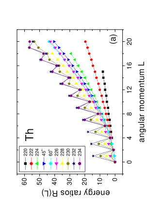
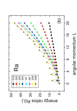
Figure 2: (color online) (a) Experimental energy ratios $R(L)=E(L)/E(2_{1}^{+})$ for ²²⁰Th [27], ²²²Th [28], ²²⁴Th [29], ²²⁶Th [30], ²²⁸Th [31], ²³⁰Th [32], ²³²Th [32, 33], and ²³⁴Th [32], compared to theoretical predictions for $\phi=45^{\rm o}$ and $\phi=60^{\rm o}$. (b) Same for ²¹⁸Ra [34, 35], ²²⁰Ra [27], ²²²Ra [32, 36], ²²⁴Ra [32, 36], ²²⁶Ra [32, 36], and ²²⁸Ra [32], compared to theoretical predictions for $\phi=45^{\rm o}$ and $\phi=56^{\rm o}$.

Experimental data for the ground state and related negative parity bands of ^220-234Th are shown in Fig. 2(a). It is clear that ²²⁶Th lies on the border between two different regions. Below ²²⁶Th the odd–even staggering is very small, while from ²²⁸Th up the odd–even staggering is becoming much larger, increasing with the neutron number $N$. A quantitative measure of the odd–even staggering and related figures can be found in Ref. [37]. It is clear that below ²²⁶Th the situation corresponds to octupole deformation, in which the ground state band and the negative parity band merge into a single band, while above ²²⁶Th the picture is corresponding to octupole vibrations, i.e. the negative parity band is a rotational band built on an octupole bandhead, thus lying systematically higher than the ground state band. Theoretical predictions for $\phi=45^{\rm o}$ lie a little below ²²⁶Th, while the $\phi=60^{\rm o}$ results follow the ²²⁶Th data very closely. It is worth remarking that the procedure of Ref. [20], which is quite different from the present one, also leads to the identification of ²²⁶Th as the nucleus lying closest to the transition point from octupole deformation to octupole vibrations.

A similar picture is observed in ^218-228Ra, shown in Fig. 2(b). In this case octupole deformation appears below ²²⁶Ra, while ²²⁸Ra is already in the regime of octupole vibrations. Theoretical predictions for $\phi_{0}=45^{\rm o}$ again lie a little below ²²⁶Ra, while the ²²⁶Ra data are followed quite closely by the predictions of $\phi_{0}=56^{\rm o}$.

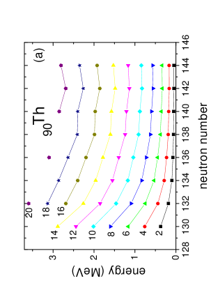
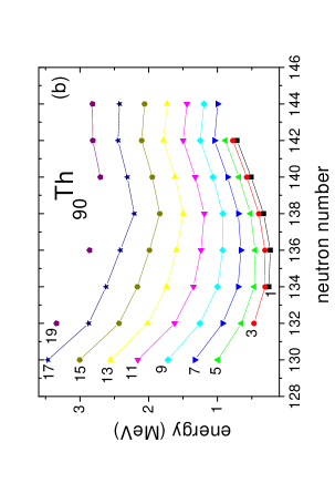
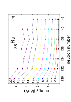
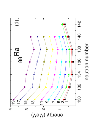
Figure 3: (color online) (a) Experimental energy levels of the ground state bands of ²²⁰Th [27], ²²²Th [28], ²²⁴Th [29], ²²⁶Th [30], ²²⁸Th [31], ²³⁰Th [32], ²³²Th [32, 33], and ²³⁴Th [32], as a function of the neutron number. (b) Same as (a), but for the associated negative parity bands. (c) Same as (a), but for ²¹⁸Ra [34, 35], ²²⁰Ra [27], ²²²Ra [32, 36], ²²⁴Ra [32, 36], ²²⁶Ra [32, 36], ²²⁸Ra [32], and ²³⁰Ra [32]. (d) Same as (c), but for the associated negative parity bands.

The behavior observed in Fig. 2(a) can be better understood by considering Figs. 3(a) and 3(b), where the experimental energy levels of the ground state band and the associated octupole band are shown, for the same thorium isotopes. While the even parity levels, shown in Fig. 3(a), smoothly decrease with increasing neutron number $N$, as a result of increasing quadrupole collectivity, the odd parity levels, shown in Fig. 3(b), exhibit a minimum, which is located at $N=136$ up to $L=9$, while it moves to $N=138$ for higher $L$. This change of behavior is then attributed to the octupole degree of freedom, showing that ${}^{226}_{90}$Th₁₃₆ lies near the border between octupole deformation and octupole vibrations. The change of behavior is not abrupt, since the effect due to octupole deformation is “moderated” by the quadrupole deformation setting in in parallel.

In a similar manner the behavior observed in Fig. 2(b) can be clarified by considering Figs. 3(c) and 3(d), where the experimental data for the same radium isotopes are presented. Again, the even parity levels decrease with increasing $N$, while the odd parity levels exhibit a minimum, located at $N=136$ up to $L=5$, while it moves to $N=138$ for higher $L$, showing that ${}^{226}_{88}$Ra₁₃₈ lies close to the border between the regions of octupole deformation and octupole vibrations.

The transition from octupole deformation to octupole vibrations can also be seen by considering the simplest quantity measuring the relative displacement of the negative parity levels with respect to the even parity ones,

$$\Delta E(L)=E(L)-{E(L-1)+E(L+1)\over 2}.$$ (33)

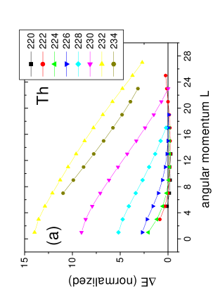
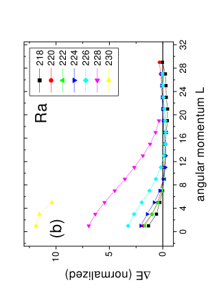
Figure 4: (color online) (a) Experimental energy staggering $\Delta E$ (Eq. (33)), normalized to the $2_{1}^{+}$ state of each nucleus, for ²²⁰Th [27], ²²²Th [28], ²²⁴Th [29], ²²⁶Th [30], ²²⁸Th [31], ²³⁰Th [32], ²³²Th [32, 33], and ²³⁴Th [32], as a function of the angular momentum. (b) Same as (a), but for ²¹⁸Ra [34, 35], ²²⁰Ra [27], ²²²Ra [32, 36], ²²⁴Ra [32, 36], ²²⁶Ra [32, 36], ²²⁸Ra [32], and ²³⁰Ra [32].

Results for the Th and Ra isotopes are shown in Figs. 4(a) and 4(b), respectively. In Fig. 4(a) it is clear that in ^222-226Th the staggering is decreasing rapidly with increasing angular momentum, reaching a vanishing value and staying close to it, which is the hallmark of octupole deformation [2, 38], while in ^228-234Th the decrease is much slower and vanishing values, if any, correspond to very high angular momenta, a behavior expected for octupole vibrations. Again ²²⁶Th appears closest to the border between the two regions. In Fig. 4(b), ^220-226Ra exhibit the rapid decrease of staggering and the sticking to values close to zero beyond the first vanishing value, while ^228-230Ra follow the slow decrease pattern. As a result, ²²⁶Ra appears to be closest to the border line between the two regions.

As far as the $0_{2}^{+}$ bandhead is concerned, the experimental values (normalized to the $2_{1}^{+}$ state) are 12.186 for ²²⁶Ra and 11.152 for ²²⁶Th, in good agreement with the 11.226 and 12.410 values predicted by the AQOA model for the $\phi_{0}$ values of $56^{\rm o}$ and $60^{\rm o}$ used in Fig. 2 . (The model of Ref. [20] provides a value of 8.528 for ²²⁶Th.) It should be noticed that the normalized $0_{2}^{+}$ bandhead is lying close to this height for all Ra and Th isotopes for which data exist, namely ²²²Ra (8.225), ²²⁴Ra (10.861), ²²⁸Ra (11.300), ²²⁸Th (14.402), ²³⁰Th (11.934), ²³²Th (14.794), ²³⁴Th (16.347), with data taken from the references used in Fig. 2 .

Considering the AQOA model as an extension of the X(5) framework involving negative parity states, as remarked at the end of Section 3, implies that the search for X(5)-like nuclei in the light actinides, where the presence of low-lying negative parity bands is important, should be focused on nuclei with $R(4)$ ratio close to 3.0 and $0_{2}^{+}$ bandhead higher than the X(5) value of 5.65 .

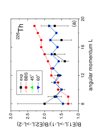
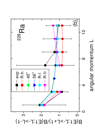
Figure 5: (color online) (a) Experimental $B(E1;L\to L-1)$ / $B(E2;L\to L-2)$ ratios (multiplied by $10^{5}$) [20] of $B(E1)$ and $B(E2)$ values originating from the same level of ²²⁶Th, compared to theoretical predictions by Bizzeti and Bizzeti-Sona [20] (labeled as BBS), as well as to predictions of the present work for $\phi_{0}=45^{\rm o}$, $60^{\rm o}$. The ratios corresponding to $L=10$ and 11 have been used for normalization, as in Ref. [20]. (b) Experimental $B(E1;L\to L+1)$ / $B(E1;L\to L-1)$ ratios [40] of $B(E1)$ values originating from the same level of ²²⁶Ra, compared to three different theoretical predictions from Ref. [39] (labeled as R-h, R-I, R-II), as well as to theoretical predictions of the present work for $\phi_{0}=45^{\rm o}$, $56^{\rm o}$. See section 4 for further discussion.

Detailed comparisons to $B(EL)$ transition rates are not feasible, because of lack of experimental data. We therefore use ratios of $B(EL)$ transitions, also used in earlier work [20, 39]. Thus in Table 5 and Fig. 5(a) the experimental $B(E1;L\to L-1)/B(E2;L\to L-2)$ ratios used in Ref. [20] are shown, together with theoretical predictions from the same source, and predictions for $\phi=45^{\rm o}$ and $60^{\rm o}$, the values also used in Fig. 2(a). The present theoretical predictions for the two different values of $\phi_{0}$ practically coincide (indicating that the predictions are essentially parameter free) and are in most cases within the error bars of the experimental points, while the predictions of Ref. [20] grow a little faster as a function of angular momentum.

Furthermore, in Table 6 and Fig. 5(b) the experimental $B(E1;L\to L+1)/B(E1;L\to L-1)$ ratios [40] used in Ref. [39] are shown, together with three sets of theoretical predictions in the framework of the extended coherent states model (ECSM) [41] from the same source, corresponding to the lowest order choice for the $E1$ transition operator (R-h), as well as to two different choices of the $E1$ transition operator, including anharmonic terms assumed suitable for the transition region (R-I, R-II) [39]. In addition, predictions for $\phi_{0}=45^{\rm o}$ and $56^{\rm o}$, the same values used in Fig. 2(b), are shown. It is clear that the predictions for the two different values of $\phi_{0}$ practically coincide (indicating that the predictions are essentially parameter free) and in all cases are within the error bars of the experimental points, being in very close agreement to the R-I predictions of Ref. [39].

On the results presented in this section, the following additional comments apply.

1) Figs. 2 and 5 indicate that ²²⁶Th (²²⁶Ra) can be well described using the AQOA model with $\phi_{0}=60^{\rm o}$ ($\phi_{0}=56^{\rm o}$), which provides results quite similar to the $\phi_{0}=45^{\rm o}$ case. In all these cases, Eq. (7) [together with Eq. (5)] indicates that the quadrupole and octupole deformations are present in comparable amounts. This is in agreement with Strutinsky-type potential-energy calculations [6, 42], resulting in comparable $\beta_{2}$ and $\beta_{3}$ values for these nuclei. The presence of octupole deformation in ²²⁶Ra has also been realized in a study [43] within the framework of the spdf-IBM [9, 10].

2) Figs. 2-4 suggest that ²²⁶Th and ²²⁶Ra lie close to the border between octupole deformation and octupole vibrations. This is in agreement with Woods–Saxon–Bogolyubov cranking calculations [7] for the Ra and Th isotopes, suggesting shape changes from nearly spherical ($N\simeq 130$) to octupole-deformed ($N\simeq 134$) to well-deformed reflection-symmetric ($N\simeq 140$) shapes, in which negative-parity bands can be interpreted in terms of octupole vibrations.

3) One can easily see that no odd–even staggering is predicted by the AQOA model. This is in agreement to the well known fact that odd-even staggering is produced when the potential in $\beta_{3}$ is a double well with two symmetric minima [44], the staggering being sensitive to the angular momentum dependence of the height of the potential barrier [45]. An infinitely high barrier leads to no odd-even staggering [44], which is indeed the case here. The introduction of a finite barrier in the present model will lead to staggering, but it will require the addition of at least one new parameter, in contrast to the main goal of the present work, which is the description of the border between octupole deformation and octupole vibrations with the minimum number of parameters possible. As shown in Figs. 2(a) and 2(b), the model does predict the border between the regions of octupole deformation and octupole vibrations in an essentially parameter independent way.

4) It should be noticed that the transition examined here is the one from octupole deformation to octupole vibrations as a function of the neutron number in a chain of isotopes, which is different from the gradual setting in of octupole deformation as a function of angular momentum in a given nucleus, usually studied by considering the odd-even staggering [2, 38], as already discussed in relation to Fig. 4.

5. The variational procedure

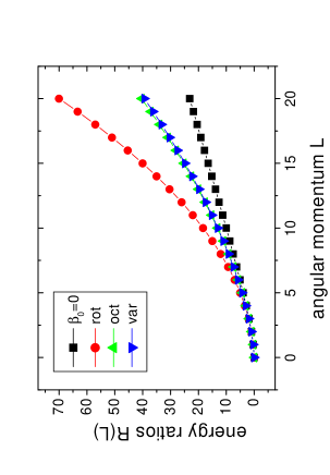
Figure 6: (color online) Energy ratios $R(L)=E(L)/E(2)$ for the ground state band and the associated negative parity band ($s=1$) of the Davidson potentials of Eq. (16), selected through the variational procedure of section 5 (labeled by “var”), compared to the ratios provided by the present work (labeled as “oct”), as a function of angular momentum. The limiting cases corresponding to Davidson potentials with $\beta_{0}=0$ (labeled as “$\beta_{0}=0$”) and $\beta_{0}\to\infty$ (labeled as “rot”) are also shown for comparison. In all cases, $\phi_{0}=45^{\rm o}$ has been used. See section 5 for further discussion.

In Refs. [18, 19] a variational procedure has been introduced, leading from the results of one-parameter Davidson potentials to the parameter-free E(5) and X(5) predictions. The same procedure can be applied in the present case, by considering (for given $\phi_{0}$) the $R(L)=E(L)/E(2)$ ratios predicted by the Davidson potentials of Eq. (16) for the excitation energies of the ground state band and the associated negative parity band, and determining for each value of $L$ separately the value of the parameter $\beta_{0}$ at which the derivative of the ratio $R(L)$ with respect to $\beta_{0}$ has a sharp maximum. The collection of $R(L)$ values selected in this way (for the case of $\phi=45^{\rm o}$) is shown in Table 7 and Fig. 6, together with the limiting cases of $\beta_{0}=0$ (a vibrator) and $\beta_{0}\to\infty$ (a rigid rotor). It is clear that the collection created through the variational procedure practicaly coincides with the predictions of the present model utilizing an infinite well potential, thus indicating that the choice of the infinite well potential indeed correponds to the transition point between a vibrator ($\beta_{0}=0$) and a rigid rotor ($\beta_{0}\to\infty$), since it is at the transition point that the rate of change of the $R(L)$ ratios is expected to become maximum.

6. Discussion

The analytic quadrupole octupole axially symmetric (AQOA) model introduced in this work describes well the border between octupole deformation and octupole vibrations in the light actinides, which corresponds to ²²⁶Th and ²²⁶Ra in the Th and Ra isotopic chains respectively. Some of the main ingredients of the present model, such as the infinite well potential and the approximate separation of variables, strongly resemble the ones used in the X(5) model, describing the critical point of the shape phase transition from vibrational to axially deformed rotational nuclei [14], determined through the study of potential energy surfaces derived from the Hamiltonian of the Interacting Boson Model [46]. An interesting task is the study of the potential energy surfaces resulting in the spdf-IBM [9, 10], the version of IBM including the octupole degree of freedom in addition to the quadrupole one, which can possibly lead to the determination of a shape phase transition from octupole deformation to octupole vibrations, in a manner similar to the determination of the critical point between the spherical and triaxial shapes found recently through the study of the potential energy surfaces resulting from an IBM-2 Hamiltonian [47, 48]. Although some early results are given in Ref. [10], this task is far from complete. The persistence of axial symmetry, as well as the importance of parity projection in this context have been emphasized [49, 50]. The inclusion of staggering in the present model, as well as its application to the rare earth region near $A=150$, where octupole deformation is known to occur [4, 5], are also of interest.

Acknowledgements

Enlightening discussions with Professor F. Iachello are gratefully acknowledged.

Table 1: Spectra of the AQOA model for the ground state band and the associated negative parity band ($s=1$), as well as for the first excited band ($s=2$) and the second excited band ($s=3$), normalized to the energy of the $2_{1}^{+}$ state, for different values of $\phi_{0}$. The second column contains the values obtained slightly above $0^{\rm o}$ or slightly below $90^{\rm o}$. In addition, the X(5) spectrum is shown for comparison. See Section 3 for further discussion.

$\phi_{0}$	$0^{\rm o}$, $90^{\rm o}$	$15^{\rm o}$	$30^{\rm o}$	$45^{\rm o}$	$60^{\rm 0}$	$75^{\rm o}$	X(5)
$L^{\pi}$
$s=1$
$0^{+}$	0.000	0.000	0.000	0.000	0.000	0.000	0.000
$1^{-}$	0.333	0.337	0.344	0.346	0.342	0.336
$2^{+}$	1.000	1.000	1.000	1.000	1.000	1.000	1.000
$3^{-}$	2.000	1.969	1.921	1.912	1.938	1.981
$4^{+}$	3.333	3.221	3.069	3.039	3.119	3.264	2.904
$5^{-}$	5.000	4.734	4.414	4.351	4.513	4.832
$6^{+}$	7.000	6.490	5.935	5.829	6.098	6.667	5.430
$7^{-}$	9.333	8.471	7.620	7.459	7.857	8.755
$8^{+}$	12.000	10.666	9.459	9.233	9.779	11.082	8.483
$9^{-}$	15.000	13.065	11.445	11.144	11.857	13.635
$10^{+}$	18.333	15.659	13.574	13.187	14.082	16.406	12.027
$11^{-}$	22.000	18.443	15.841	15.359	16.451	19.386
$12^{+}$	26.000	21.410	18.245	17.658	18.959	22.567	16.041
$13^{-}$	30.333	24.557	20.782	20.081	21.605	25.943
$14^{+}$	35.000	27.881	23.452	22.626	24.384	29.510	20.514
$15^{-}$	40.000	31.379	26.251	25.293	27.297	33.264
$16^{+}$	45.333	35.048	29.180	28.080	30.340	37.200	25.437
$17^{-}$	51.000	38.886	32.237	30.985	33.513	41.315
$18^{+}$	57.000	42.892	35.421	34.009	36.814	45.607	30.804
$19^{-}$	63.333	47.064	38.731	37.150	40.242	50.074
$20^{+}$	70.000	51.402	42.166	40.408	43.796	54.713	36.611
$s=2$
$0^{+}$		13.292	8.983	9.351	12.410	23.896	5.649
$2^{+}$		14.893	10.726	11.133	14.160	25.502	7.450
$4^{+}$		18.384	14.204	14.630	17.763	29.098	10.689
$6^{+}$		23.392	18.820	19.209	22.649	34.410	14.751
$s=3$
$0^{+}$		30.940	21.944	23.114	30.316	55.625	14.119

Table 2: $B(E2;L_{i}\to L_{f})$ values between states of the AQOA model with $s=1$. $B(E2)$s with $L_{i}$ and $L_{f}$ even are normalized to the $2_{1}^{+}\to 0_{1}^{+}$ transition, while $B(E2)$s with $L_{i}$ and $L_{f}$ odd are normalized to the $3_{1}^{-}\to 1_{1}^{-}$ transition. The X(5) results are also shown for comparison. See Section 3 for further discussion.

	$\phi_{0}$	$1^{\rm o}$	$15^{\rm o}$	$30^{\rm o}$	$45^{\rm o}$	$60^{\rm 0}$	$75^{\rm o}$	X(5)
$L_{i}^{\pi}$	$L_{f}^{\pi}$
$2^{+}$	$0^{+}$	1.000	1.000	1.000	1.000	1.000	1.000	1.000
$4^{+}$	$2^{+}$	1.429	1.475	1.530	1.539	1.509	1.457	1.599
$6^{+}$	$4^{+}$	1.574	1.701	1.834	1.855	1.786	1.656	1.982
$8^{+}$	$6^{+}$	1.648	1.870	2.072	2.104	2.005	1.797	2.276
$10^{+}$	$8^{+}$	1.693	2.011	2.268	2.309	2.187	1.915	2.509
$12^{+}$	$10^{+}$	1.723	2.131	2.431	2.480	2.342	2.019	2.697
$14^{+}$	$12^{+}$	1.746	2.236	2.569	2.626	2.476	2.111	2.854
$16^{+}$	$14^{+}$	1.762	2.327	2.687	2.751	2.593	2.194	2.987
$18^{+}$	$16^{+}$	1.776	2.407	2.790	2.860	2.695	2.269	3.101
$20^{+}$	$18^{+}$	1.787	2.478	2.881	2.955	2.785	2.337	3.200
$3^{-}$	$1^{-}$	1.000	1.000	1.000	1.000	1.000	1.000
$5^{-}$	$3^{-}$	1.179	1.227	1.278	1.286	1.260	1.210
$7^{-}$	$5^{-}$	1.257	1.374	1.479	1.496	1.444	1.335
$9^{-}$	$7^{-}$	1.301	1.491	1.642	1.665	1.595	1.433
$11^{-}$	$9^{-}$	1.329	1.591	1.777	1.806	1.723	1.518
$13^{-}$	$11^{-}$	1.350	1.677	1.890	1.924	1.832	1.594
$15^{-}$	$13^{-}$	1.365	1.752	1.986	2.026	1.927	1.661
$17^{-}$	$15^{-}$	1.376	1.817	2.069	2.114	2.010	1.722
$19^{-}$	$17^{-}$	1.386	1.875	2.142	2.190	2.082	1.777

Table 3: $B(E1;L_{i}\to L_{f})$ values between states with $s=1$, normalized to the $1_{1}^{-}\to 0_{1}^{+}$ transition.

	$\phi_{0}$	$1^{\rm o}$	$15^{\rm o}$	$30^{\rm o}$	$45^{\rm o}$	$60^{\rm 0}$	$75^{\rm o}$
$L_{i}^{\pi}$	$L_{f}^{\pi}$
$1^{-}$	$0^{+}$	1.000	1.000	1.000	1.000	1.000	1.000
$2^{+}$	$1^{-}$	1.200	1.227	1.264	1.269	1.247	1.215
$3^{-}$	$2^{+}$	1.286	1.358	1.455	1.469	1.414	1.328
$4^{+}$	$3^{-}$	1.334	1.467	1.633	1.657	1.564	1.413
$5^{-}$	$4^{+}$	1.364	1.570	1.807	1.842	1.712	1.489
$6^{+}$	$5^{-}$	1.385	1.670	1.977	2.022	1.857	1.562
$7^{-}$	$6^{+}$	1.401	1.768	2.141	2.196	2.000	1.634
$8^{+}$	$7^{-}$	1.413	1.864	2.299	2.364	2.139	1.705
$9^{-}$	$8^{+}$	1.423	1.957	2.449	2.523	2.273	1.777
$10^{+}$	$9^{-}$	1.431	2.048	2.592	2.676	2.403	1.847
$11^{-}$	$10^{+}$	1.437	2.135	2.727	2.821	2.527	1.917
$12^{+}$	$11^{-}$	1.443	2.220	2.856	2.959	2.646	1.985
$13^{-}$	$12^{+}$	1.448	2.300	2.979	3.090	2.760	2.052
$14^{+}$	$13^{-}$	1.452	2.377	3.095	3.215	2.870	2.117
$15^{-}$	$14^{+}$	1.456	2.451	3.206	3.334	2.974	2.181
$16^{+}$	$15^{-}$	1.460	2.522	3.311	3.447	3.075	2.242
$17^{-}$	$16^{+}$	1.463	2.590	3.411	3.555	3.171	2.302
$18^{+}$	$17^{-}$	1.466	2.655	3.507	3.659	3.263	2.360
$19^{-}$	$18^{+}$	1.469	2.718	3.598	3.757	3.351	2.417
$20^{+}$	$19^{-}$	1.471	2.778	3.685	3.852	3.436	2.471

Table 4: $B(E3;L_{i}\to L_{f})$ values between states with $s=1$, normalized to the $3_{1}^{-}\to 0_{1}^{+}$ transition.

	$\phi_{0}$	$1^{\rm o}$	$15^{\rm o}$	$30^{\rm o}$	$45^{\rm o}$	$60^{\rm 0}$	$75^{\rm o}$
$L_{i}^{\pi}$	$L_{f}^{\pi}$
$3^{-}$	$0^{+}$	1.000	1.000	1.000	1.000	1.000	1.000
$4^{+}$	$1^{-}$	1.333	1.351	1.369	1.373	1.364	1.345
$5^{-}$	$2^{+}$	1.515	1.563	1.613	1.623	1.596	1.547
$6^{+}$	$3^{-}$	1.632	1.719	1.809	1.825	1.778	1.690
$7^{-}$	$4^{+}$	1.714	1.847	1.979	2.001	1.934	1.804
$8^{+}$	$5^{-}$	1.774	1.958	2.130	2.158	2.073	1.900
$9^{-}$	$6^{+}$	1.821	2.058	2.267	2.300	2.199	1.986
$10^{+}$	$7^{-}$	1.859	2.149	2.390	2.429	2.314	2.063
$11^{-}$	$8^{+}$	1.889	2.233	2.502	2.546	2.420	2.135
$12^{+}$	$9^{-}$	1.915	2.310	2.605	2.653	2.517	2.202
$13^{-}$	$10^{+}$	1.936	2.381	2.699	2.752	2.607	2.264
$14^{+}$	$11^{-}$	1.955	2.447	2.786	2.842	2.691	2.323
$15^{-}$	$12^{+}$	1.971	2.509	2.865	2.926	2.768	2.379
$16^{+}$	$13^{-}$	1.985	2.567	2.939	3.004	2.841	2.431
$17^{-}$	$14^{+}$	1.998	2.621	3.008	3.076	2.908	2.481
$18^{+}$	$15^{-}$	2.009	2.671	3.072	3.143	2.971	2.528
$19^{-}$	$16^{+}$	2.019	2.719	3.132	3.207	3.031	2.573
$20^{+}$	$17^{-}$	2.028	2.763	3.188	3.266	3.087	2.615
$2^{+}$	$1^{-}$	1.800	1.794	1.797	1.797	1.793	1.795
$3^{-}$	$2^{+}$	1.333	1.353	1.386	1.390	1.370	1.344
$4^{+}$	$3^{-}$	1.273	1.321	1.383	1.391	1.356	1.301
$5^{-}$	$4^{+}$	1.259	1.338	1.429	1.441	1.393	1.308
$6^{+}$	$5^{-}$	1.257	1.370	1.486	1.503	1.442	1.329
$7^{-}$	$6^{+}$	1.258	1.406	1.545	1.565	1.495	1.355
$8^{+}$	$7^{-}$	1.261	1.443	1.602	1.625	1.547	1.383
$9^{-}$	$8^{+}$	1.264	1.480	1.656	1.683	1.598	1.413
$10^{+}$	$9^{-}$	1.267	1.516	1.707	1.736	1.646	1.442
$11^{-}$	$10^{+}$	1.270	1.550	1.754	1.786	1.691	1.471
$12^{+}$	$11^{-}$	1.272	1.582	1.798	1.833	1.734	1.498
$13^{-}$	$12^{+}$	1.275	1.612	1.840	1.876	1.774	1.526
$14^{+}$	$13^{-}$	1.277	1.641	1.878	1.917	1.812	1.552
$15^{-}$	$14^{+}$	1.279	1.669	1.914	1.955	1.848	1.577
$16^{+}$	$15^{-}$	1.281	1.695	1.948	1.991	1.881	1.601
$17^{-}$	$16^{+}$	1.283	1.719	1.979	2.025	1.913	1.624
$18^{+}$	$17^{-}$	1.285	1.742	2.009	2.056	1.943	1.646
$19^{-}$	$18^{+}$	1.287	1.764	2.037	2.086	1.971	1.667
$20^{+}$	$19^{-}$	1.288	1.785	2.064	2.114	1.998	1.688

Table 5: Experimental $B(E1;L\to L-1)$ / $B(E2;L\to L-2)$ ratios (multiplied by $10^{5}$) [20] of $B(E1)$ and $B(E2)$ values originating from the same level of ²²⁶Th, compared to theoretical predictions for $\phi_{0}=45^{\rm o}$, $60^{\rm o}$, as well as to theoretical predictions by Bizzeti and Bizzeti-Sona [20] (labeled as BBS). As in Ref. [20], asterisks indicate the values used for normalization.

$L^{\pi}$	exp	$45^{\rm o}$	$60^{\rm o}$	BBS
$8^{+}$	2.0 (8)	1.454	1.457	1.3
$9^{-}$	1.7 (2)	1.649	1.652	1.3
$10^{+}$	1.5 (1)∗	1.500∗	1.500∗	1.6∗
$11^{-}$	1.7 (1)∗	1.700∗	1.700∗	1.6∗
$12^{+}$	1.6 (1)	1.544	1.542	1.8
$13^{-}$		1.747	1.746	1.8
$14^{+}$	1.4 (1)	1.585	1.582	1.9
$15^{-}$	1.7 (3)	1.791	1.789	2.0
$16^{+}$		1.622	1.619	2.1
$17^{-}$	1.5 (3)	1.831	1.829	2.1
$18^{+}$		1.656	1.653	2.2
$19^{-}$	1.7 (4)	1.867	1.865	2.3

Table 6: Experimental $B(E1;L\to L+1)$ / $B(E1;L\to L-1)$ ratios [40] of $B(E1)$ values originating from the same level of ²²⁶Ra, compared to theoretical predictions for $\phi_{0}=45^{\rm o}$, $56^{\rm o}$, as well as to three different theoretical predictions from Ref. [39], labelled as R-h, R-I, R-II. See section 4 for further discussion.

$L^{\pi}$	exp	$45^{\rm o}$	$56^{\rm o}$	R-h	R-I	R-II
$1^{-}$	1.85$\pm$1.20	2.116	2.092	1.84	1.98	1.85
$3^{-}$	0.87$\pm$0.35	1.451	1.433	1.12	1.31	0.95
$5^{-}$		1.297	1.288
$7^{-}$	1.79$\pm$1.59	1.220	1.215	0.86	1.12	0.99
$9^{-}$	1.27$\pm$0.68	1.172	1.170	0.83	1.10	1.13
$11^{-}$	1.12$\pm$0.79	1.140	1.139	0.83	1.10	1.26
$13^{-}$	1.06$\pm$0.68	1.117	1.117	0.85	1.11	1.35

Table 7: Parameter values $\beta_{0,max}$ where the first derivative of the energy ratios $R(L)=E(L)/E(2)$ for the ground state band and the associated negative parity band ($s=1$) of the Davidson potentials of Eq. (16) has a maximum, while the second derivative vanishes, together with the $R(L)$ ratios obtained at these values (labeled by “var”) and the corresponding ratios of the present model (labeled by “oct”), for several values of the angular momentum $L$. In all cases $\phi_{0}=45^{\rm o}$ has been used. See section 5 for further discussion.

$L^{\pi}$	$\beta_{0,max}$	$R_{L}$	$R_{L}$
		var	oct
$1^{-}$	1.200	0.347	0.346
$2^{+}$		1.000	1.000
$3^{-}$	1.283	1.909	1.912
$4^{+}$	1.329	3.030	3.039
$5^{-}$	1.374	4.333	4.351
$6^{+}$	1.419	5.797	5.829
$7^{-}$	1.461	7.407	7.459
$8^{+}$	1.502	9.154	9.233
$9^{-}$	1.541	11.032	11.144
$10^{+}$	1.579	13.034	13.187

References

- [1] A. Bohr and B. R. Mottelson, Nuclear Structure, Vol. II (Benjamin, New York, 1975).
- [2] P. Schüler, Ch. Lauterbach, Y. K. Agarwal, J. De Boer, K. P. Blume, P. A. Butler, K. Euler, Ch. Fleischmann, C. Günther, E. Hauber, H. J. Maier, M. Marten-Tölle, Ch. Schandera, R. S. Simon, R. Tölle, and P. Zeyen, Phys. Lett. B 174, 241 (1986).
- [3] S. G. Rohoziński, Rep. Prog. Phys. 51, 541 (1988).
- [4] I. Ahmad and P. A. Butler, Annu. Rev. Nucl. Part. Sci. 43, 71 (1993).
- [5] P. A. Butler and W. Nazarewicz, Rev. Mod. Phys. 68, 349 (1996).
- [6] W. Nazarewicz, P. Olanders, I. Ragnarsson, J. Dudek, G. A. Leander, P. Möller, and E. Ruchowska, Nucl. Phys. A 429, 269 (1984).
- [7] W. Nazarewicz and P. Olanders, Nucl. Phys. A 441, 420 (1985).
- [8] R. K. Sheline, Phys. Lett. B 197, 500 (1987).
- [9] J. Engel and F. Iachello, Phys. Rev. Lett. 54, 1126 (1985).
- [10] J. Engel and F. Iachello, Nucl. Phys. A 472, 61 (1987).
- [11] H. J. Daley and F. Iachello, Ann. Phys. (N.Y.) 167, 73 (1986).
- [12] B. Buck, A. C. Merchant, and S. M. Perez, Phys. Rev. C 57, R2095 (1998).
- [13] T. M. Shneidman, G. G. Adamian, N. V. Antonenko, R. V. Jolos, and W. Scheid, Phys. Rev. C 67, 014313 (2003).
- [14] F. Iachello, Phys. Rev. Lett. 87, 052502 (2001).
- [15] F. Iachello, Phys. Rev. Lett. 85, 3580 (2000).
- [16] A. Ya. Dzyublik and V. Yu. Denisov, Yad. Fiz. 56, 30 (1993) [Phys. At. Nucl. 56, 303 (1993)].
- [17] P. M. Davidson, Proc. R. Soc. London Ser. A 135, 459 (1932).
- [18] D. Bonatsos, D. Lenis, N. Minkov, D. Petrellis, P. P. Raychev, and P. A. Terziev, Phys. Lett. B 584, 40 (2004).
- [19] D. Bonatsos, D. Lenis, N. Minkov, D. Petrellis, P. P. Raychev, and P. A. Terziev, Phys. Rev. C 70, 024305 (2004).
- [20] P. G. Bizzeti and A. M. Bizzeti-Sona, Phys. Rev. C 70, 064319 (2004).
- [21] A. S. Davydov and A. A. Chaban, Nucl. Phys. 20, 499 (1960).
- [22] V. Yu. Denisov and A. Ya. Dzyublik, Nucl. Phys. A 589, 17 (1995).
- [23] J. P. Elliott, J. A. Evans, and P. Park, Phys. Lett. B 169, 309 (1986).
- [24] D. J. Rowe and C. Bahri, J. Phys. A 31, 4947 (1998).
- [25] P. Holmberg and P. O. Lipas, Nucl. Phys. A 117, 552 (1968).
- [26] A. R. Edmonds, Angular Momentum in Quantum Mechanics (Princeton University Press, Princeton, 1957).
- [27] A. Artna-Cohen, Nucl. Data Sheets 80, 157 (1997).
- [28] Y. A. Akovali, Nucl. Data Sheets 77, 271 (1996).
- [29] A. Artna-Cohen, Nucl. Data Sheets 80, 227 (1997).
- [30] Y. A. Akovali, Nucl. Data Sheets 77, 433 (1996).
- [31] A. Artna-Cohen, Nucl. Data Sheets 80, 723 (1997).
- [32] J. F. C. Cocks, D. Hawcroft, N. Amzal, P. A. Butler, K. J. Cann, P. T. Greenlees, G. D. Jones, S. Asztalos, R. M. Clark, M. A. Deleplanque, R. M. Diamond, P. Fallon, I. Y. Lee, A. O. Macchiavelli, R. W. MacLeod, F. S. Stephens, P. Jones, R. Julin, R. Broda, B. Fornal, J. F. Smith, T. Lauritsen, P. Bhattacharyya, and C. T. Zhang, Nucl. Phys. A 645, 61 (1999).
- [33] M. R. Schmorak, Nucl. Data Sheets 63, 139 (1991).
- [34] Y. A. Akovali, Nucl. Data Sheets 76, 457 (1995).
- [35] N. Schulz, V. Vanin, M. Aïche, A. Chevallier, J. Chevallier, J. C. Sens, Ch. Briançon, S. Cwiok, E. Ruchowska, J. Fernandez-Niello, Ch. Mittag, and J. Dudek, Phys. Rev. Lett. 63, 2645 (1989).
- [36] J. F. C. Cocks, P. A. Butler, K. J. Cann, P. T. Greenlees, G. D. Jones, S. Asztalos, P. Bhattacharyya, R. Broda, R. M. Clark, M. A. Deleplanque, R. M. Diamond, P. Fallon, B. Fornal, P. M. Jones, R. Julin, T. Lauritsen, I. Y. Lee, A. O. Macchiavelli, R. W. MacLeod, J. F. Smith, F. S. Stephens, and C. T. Zhang, Phys. Rev. Lett. 78, 2920 (1997).
- [37] D. Bonatsos, C. Daskaloyannis, S. B. Drenska, N. Karoussos, N. Minkov, P. P. Raychev, and R. P. Roussev, Phys. Rev. C 62, 024301 (2000).
- [38] W. R. Phillips, I. Ahmad, H. Emling, R. Holzmann, R. V. F. Janssens, T.-L. Khoo, and M. W. Drigert, Phys. Rev. Lett. 57, 3257 (1986).
- [39] A. A. Raduta, D. Ionescu, I. I. Ursu, and A. Faessler, Nucl. Phys. A 720, 43 (2003).
- [40] H. J. Wollersheim, H. Emling, H. Grein, R. Kulessa, R. S. Simon, C. Fleischmann, J. de Boer, E. Hauber, C. Lauterbach, C. Schandera, P. A. Butler, and T. Czosnyka, Nucl. Phys. A 556, 261 (1993).
- [41] A. A. Raduta, Recent Res. Devel. Nuclear Phys. 1, 1 (2004).
- [42] G. A. Leander, W. Nazarewicz, G. F. Bertsch, and J. Dudek, Nucl. Phys. A 453, 58 (1986).
- [43] N. V. Zamfir and D. Kusnezov, Phys. Rev. C 63, 054306 (2001).
- [44] G. A. Leander, R. K. Sheline, P. Möller, P. Olanders, I. Ragnarsson, and A. J. Sierk, Nucl. Phys. A 388, 452 (1982).
- [45] R. V. Jolos and P. von Brentano, Phys. Rev. C 49, R2301 (1994).
- [46] F. Iachello and A. Arima, The Interacting Boson Model (Cambridge University Press, Cambridge, 1987).
- [47] J. M. Arias, J. E. García-Ramos, and J. Dukelsky, Phys. Rev. Lett. 93, 212501 (2004).
- [48] M. A. Caprio and F. Iachello, Phys. Rev. Lett. 93, 242502 (2004).
- [49] S. Kuyucak, Phys. Lett. B 466, 79 (1999).
- [50] S. Kuyucak and M. Honma, Phys. Rev. C 65, 064323 (2002).