Relativistic models for quasi-elastic neutrino scattering

Abstract

We present quasi-elastic neutrino-nucleus cross sections in the energy range from 150 MeV up to 5 GeV for the target nuclei ¹²C and ⁵⁶Fe. A relativistic description of the nuclear dynamics and the neutrino-nucleus coupling is adopted. For the treatment of final-state interactions (FSI) we rely on two frameworks succesfully applied to exclusive electron-nucleus scattering: a relativistic optical potential and a relativistic multiple-scattering Glauber approximation. At lower energies, the optical-potential approach is considered to be the optimum choice, whereas at high energies a Glauber approach is more natural. Comparing the results of both calculations, it is found that the Glauber approach yields valid results down to the remarkably small nucleon kinetic energies of 200 MeV. We argue that the nuclear transparencies extracted from $A(e,\,e^{\prime}p)$ measurements can be used to obtain realistic estimates of the effect of FSI mechanisms on quasi-elastic neutrino-nucleus cross sections. We present two independent relativistic plane-wave impulse approximation (RPWIA) calculations of quasi-elastic neutrino-nucleus cross sections. They agree at the percent level, showing the reliability of the numerical techniques adopted and providing benchmark RPWIA results.

I Introduction

Neutrino interactions offer unique opportunities for exploring fundamental questions in different domains of physics. The mass of the neutrino remains one of the greatest puzzles in elementary particle physics. In recent years, a number of positive neutrino oscillation signals made the claims of non-zero neutrino masses irrefutable superkam98 and boosted the interest in this issue. Several experiments are running or proposed in order to address intriguing questions in current neutrino physics freedman : What does the neutrino mass hierarchy look like, and what are the values of the oscillation parameters superkam98 ? What is the role of vacuum and matter-enhanced oscillations ? Are neutrinos representatives of CP-violation in the leptonic sector ? Is the neutrino a Dirac or a Majorana particle ? Does it have a magnetic moment ? minerva .

The interest in neutrinos goes beyond the study of the particle’s intrinsic properties, and extends to a variety of topics in astro-, nuclear and hadronic physics. Typical astrophysical examples include the understanding of the energy production in our sun, neutrino nucleosynthesis and the synthesis of heavy elements during the r-process, the influence of neutrinos on the dynamics of a core-collapse supernova explosion and the cooling of a proto-neutronstar bahcall ; langanke . In many astrophysical situations the neutrinos serve as messengers probing the interior of dense and opaque objects that otherwise remain inaccessible. The influence of neutrinos even extends to cosmological questions such as the role of neutrinos in the matter-antimatter asymmetry in the universe. In hadronic and nuclear physics, neutrino scattering can shed light on a lot of issues, including investigations of electroweak form factors, the study of the strange quark content of the nucleon and $\nu$-induced pion production minerva ; boone ; nutev .

Despite the richness of phenomena they are involved in, neutrinos remain elusive particles, only weakly interacting and eager to escape detectors on the watch. The presence of neutrinos, being chargeless particles, can only be inferred by detecting the secondary particles they create when colliding and interacting with matter. Nuclei are often used as neutrino detectors, providing relatively large cross sections that offer a broad variety of information. As a consequence, a reliable interpretation of data involving neutrinos heavily counts on a detailed knowledge of the magnitude of neutrino-nucleus interactions under various circumstances. A precise knowledge of the energy and mass number dependence of the neutrino-nucleus cross section is essential to current and future measurements. The energies that neutrinos can transfer to nuclei depend on their origin. The ’low’ energy regime extends to a few tens of MeV and relates to reactor, solar and supernova neutrinos. Atmospheric and accelerator neutrinos can carry energies from a few hundred MeV to several GeV’s.

At intermediate energies (here defined as energies beyond the nuclear resonance region), neutrino-nucleus interactions have been studied within several approaches, investigating a variety of effects. The relativistic Fermi gas (RFG) model was employed in Refs. horo ; umino to study the possibility of measuring strange-quark contributions to the nucleon form factors. The RFG takes into account the Fermi motion of the nucleons inside the nucleus, Pauli blocking and relativistic kinematics, but neglects several other effects. Ref. polarlet used a plane-wave impulse approximation description of the nuclear system to estimate polarization asymmetry effects in neutrino-induced nucleon knockout. Relativistic nuclear effects were included in the calculations of Refs. barbar ; albe1 ; albe2 ; mai ; meuccineut ; meuccichar ; vanderventel04 , using a relativistic shell model approach for the study of neutral-current and/or charged-current neutrino-nucleus scattering. In particular, in Refs. albe1 ; albe2 ; mai results in the relativistic plane-wave impulse approximation (RPWIA) were compared to RFG calculations. It is shown that binding-energy effects tend to vanish as the energy increases. Going one step further in the complexity of the model calculation, the implementation of the final-state interactions (FSI) of the ejected nucleon has been achieved in different manners. In Ref. bleve01 a phenomenological convolution model was applied to the RFG, showing that nucleon re-scattering can produce a reduction of the quasi-elastic cross section as large as $15\%$ at incoming neutrino energies of about 1 GeV. A description of FSI mechanisms through the inclusion of relativistic optical potentials is presented in Refs. albe1 ; albe2 ; mai ; meuccineut ; meuccichar . More specifically, Ref. mai studies the uncertainties derived from the use of different prescriptions for the potentials. A reduction of the cross section of at least $14\%$ is found at incoming neutrino energies of 1 GeV. In Refs. meuccineut ; meuccichar , important FSI effects arise from the use of relativistic optical potentials within a relativistic Green’s function approach. Apart from relativistic dynamics and FSI, other effects may have an impact on neutrino-nucleus reactions. In Refs. kim1 ; kim2 the influence of relativistic nuclear structure effects, delta- and pion degrees-of-freedom, and RPA-type correlations on neutrino-scattering cross sections was examined. Ref. nieves includes long-range correlations, FSI and Coulomb corrections in ${}^{12}C(\nu_{\mu},\mu^{-})^{12}C^{*}$ calculations. An alternative method was proposed in Ref. amaro , where it was shown that a superscaling analysis of few-GeV inclusive electron scattering data allows one to predict charged-current neutrino cross sections in the nuclear resonance region, thereby effectively including delta isobar degrees-of-freedom.

In this paper we compute the single-nucleon knockout (often referred to as quasi-elastic (QE)) contribution to the inclusive neutrino-nucleus cross sections, for energies and nuclei relevant to proposals like Miner$\nu$a minerva , Miniboone boone and Finesse finesse . We consider that the large variety of relevant neutrino energies and the tendency to study neutrino-nucleus interactions at increasing energies, necessitate the use of relativity. We employ two relativistic models for describing neutrino-nucleus scattering within the impulse approximation: the relativistic distorted-wave impulse approximation (RDWIA) developed by the Madrid-Seville group, and the relativistic multiple scattering Glauber approximation (RMSGA) developed by the Ghent group. Initially designed for the description of exclusive electron-nucleus scattering processes, both models have been succesfully tested against $A(e,e^{\prime}p)$ data Udi93 ; Udi96 ; Udi99 ; Udi01 ; cris04 ; lava04 ; lava05 . In addition, the nuclear transparencies predicted by these models have proven to be mutually consistent in the intermediate kinematic regime between 0.5 and 1 GeV nucleon kinetic energies where both of them are deemed reliable lava04 . The RDWIA model used here has already been employed in several neutrino-nucleus calculations albe1 ; albe2 ; mai . To our knowledge, this paper is the first report of a relativistic Glauber-inspired approach to neutrino-nucleus reactions. The aim of this work is twofold. First, the relativistic models available to date predict different results in the limit of vanishing FSI, motivating a ’new round’ of calculations. We investigate the plane-wave limit of the RDWIA and RMSGA approximations, aiming at providing benchmark RPWIA results. Second, we compute the effects of FSI within our models, paying special attention to the comparison between RDWIA and RMSGA results. It is well known that the inclusion of FSI within inclusive calculations requires a considerable computing effort. We propose a way to estimate FSI effects for the QE contribution to the inclusive neutrino-nucleus cross section using benchmark RPWIA results and transparency data obtained from $A(e,e^{\prime}p)$ experiments. For the time being, the effects of many-body currents, nucleon-nucleon correlations, and contributions beyond quasi-elastic scattering processes as multi-nucleon processes and pion production are neglected.

The outline of this paper is as follows. In Sec. II we present the RMSGA and RDWIA formalisms for the description of the neutral- and charged-current neutrino-nucleus scattering processes. Results of the numerical calculations are shown in Sec. III. Sec. IV summarizes our findings.

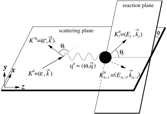
Figure 1: Kinematics for the quasi-elastic neutrino-nucleus scattering process

II Formalism

We derive expressions for neutrino and antineutrino neutral-current (NC) reactions from nuclei which result in one emitted nucleon

$$\nu(\overline{\nu})+A\Longrightarrow\nu(\overline{\nu})+N+(A-1).$$ (1)

We also consider their charged-current (CC) counterparts

$$\nu(\overline{\nu})+A\Longrightarrow l(\overline{l})+N+(A-1).$$ (2)

Here, $l$ labels the flavor of the lepton, and $A$ represents a nucleus with mass number $A$. The connection between electromagnetic and weak interactions makes that the analytical derivations follow the same lines as those used in electron-nucleus scattering. The main differences between neutrino and electron interactions stem from the intrinsic polarization of the neutrino due to the parity-violating character of the weak interaction. Moreover in weak interactions the focus is on inclusive processes, whereas exclusive processes play a predominant role in current subatomic research with electrons.

We describe these processes at lowest order in the electroweak interaction, i.e. considering the exchange of one charged vector boson. Fig. 1 defines our conventions for the kinematical variables. The four-momenta of the incident neutrino and scattered lepton are labeled $K^{\mu}$ and $K^{\prime\mu}$. Further, $K^{\mu}_{A}$, $K^{\mu}_{A-1}$ and $K^{\mu}_{f}$ represent the four-momenta of the target nucleus, the residual nucleus and the ejected nucleon. The $xyz$ coordinate system is chosen such that the $z-$axis lies along the momentum transfer $\vec{q}$, the $y-$axis along $\vec{k}\times\vec{k^{\prime}}$ and the $x-$axis lies in the scattering plane. The hadron reaction plane is then defined by $\vec{k}_{f}$ and $\vec{q}$. We adopt the standard convention $Q^{2}\equiv-q_{\mu}q^{\mu}$ for the four-momentum transfer.

II.1 Quasi-elastic neutrino-nucleus cross section

In the laboratory frame, the exclusive differential cross section for the processes specified in Eqs. (1) and (2) can be written as bjorken64

$$d\sigma=\frac{1}{\beta}\overline{\sum_{if}}|M_{fi}|^{2}\frac{M_{l}}{\varepsilon^{\prime}}\frac{M_{A-1}}{E_{A-1}}\frac{M_{N}}{E_{f}}d^{3}\vec{k}_{A-1}d^{3}\vec{k^{\prime}}d^{3}\vec{k}_{f}$$

$$\times(2\pi)^{-5}\delta^{4}(K^{\mu}+K^{\mu}_{A}-K^{\prime\mu}-K^{\mu}_{A-1}-K^{\mu}_{f}),$$ (3)

where $\overline{\sum_{if}}$ indicates sum and/or average over initial and final spins. Dealing with neutrinos, the relative initial velocity $\beta$ can trivially be put to 1. The factor $\frac{M_{l}}{\varepsilon^{\prime}}$ stems from the normalization of the outgoing lepton spinor and becomes 1 for NC reactions. Integrating over the unobserved momentum of the recoiling nucleus $\vec{k}_{A-1}$, as well as over $|\vec{k_{f}}|$, results in the following fivefold differential cross section for the $A(\nu,\nu^{\prime}N)$, $A(\overline{\nu},\overline{\nu}^{\prime}N)$, $A(\nu,lN)$ and $A(\overline{\nu},\overline{l}N)$ reactions

$$\frac{d^{5}\sigma}{d\varepsilon^{\prime}d^{2}\Omega_{l}d^{2}{\Omega_{f}}}=\frac{M_{l}M_{N}M_{A-1}}{(2\pi)^{5}M_{A}\varepsilon^{\prime}}k^{\prime 2}k_{f}f_{rec}^{-1}\overline{\sum_{if}}|M_{fi}|^{2},$$ (4)

where $\Omega_{l}$ and ${\Omega_{f}}$ define the scattering direction of the outgoing lepton and the outgoing nucleon. The recoil factor $f_{rec}$ is given by

$$f_{rec}=\frac{E_{A-1}}{M_{A}}\left|1+\frac{E_{f}}{E_{A-1}}[1-\frac{\vec{q}\cdot\vec{k}_{f}}{k_{f}^{2}}]\right|.$$ (5)

The squared invariant matrix element $M_{fi}$ can be written as

$$\overline{\sum_{if}}|M_{fi}|^{2}=\frac{G_{F}^{2}}{2}\left[\frac{M_{B}^{2}}{Q^{2}+M_{B}^{2}}\right]^{2}l_{\alpha\beta}W^{\alpha\beta}.$$ (6)

Here, $M_{B}$ represents the mass of the $Z$-boson for NC reactions and that of the $W$-boson for CC processes. $G_{F}$ is the Fermi constant. For CC reactions the latter has to be multiplied with a factor $\cos{\theta_{c}}$, with $\theta_{c}$ the Cabbibo angle, determining the mixing of the strong down and strange quarks into the weak d-quark. In the above expression the lepton tensor is defined as

$$l_{\alpha\beta}\equiv\overline{\sum_{s,s^{\prime}}}[\overline{u}_{l}\gamma_{\alpha}(1-\gamma_{5})u_{l}]^{\dagger}[\overline{u}_{\nu}\gamma_{\beta}(1-\gamma_{5})u_{\nu}],$$ (7)

with $s$ and $s^{\prime}$ the initial and final lepton spins. The hadron tensor is given by

$$W^{\alpha\beta}=\overline{\sum_{if}}\langle\Delta^{\alpha\mu}J_{\mu}\rangle^{\dagger}\langle\Delta^{\beta\nu}J_{\nu}\rangle=\overline{\sum_{if}}\langle\cal{J}^{\alpha}\rangle^{\dagger}\langle\cal{J}^{\beta}\rangle,$$ (8)

with the boson propagator

$$\Delta^{\mu\nu}=g^{\mu\nu}-\frac{q^{\mu}q^{\nu}}{M_{B}^{2}}.$$ (9)

The quantity $\langle\cal{J}^{\alpha}\rangle$ in Eq. (8) can be written as

$$\left<\cal{J}^{\alpha}\right>\equiv\left<(A-1)(J_{R}M_{R}),K_{f}(E_{f},\vec{k}_{f})m_{s}\left|\Delta_{\alpha\mu}\hat{J}^{\mu}\right|A(0^{+},g.s.)\right>,$$ (10)

with $\hat{J}^{\mu}$ the weak current operator, $\left|A(0^{+},g.s.)\right>$ the ground state of the target even-even nucleus and $\left|(A-1)(J_{R}M_{R})\right>$ the state in which the residual nucleus is left. At the energies considered here, Eq. (9) can approximately be written as $\Delta^{\mu\nu}\approx g^{\mu\nu}$, and the quantity $\langle\cal{J}^{\alpha}\rangle\approx\langle$$J^{\alpha}\rangle$, establishing the connection between the four-vector $\cal{J}^{\alpha}$ and the nuclear current operator. In the extreme relativistic limit, the contraction of the lepton tensor $l_{\alpha\beta}$ with the nuclear one $W^{\alpha\beta}$ in Eq. (6) can be cast in the form donnelly86  :

$$\frac{d^{5}\sigma}{d\varepsilon^{\prime}d^{2}\Omega_{l}d^{2}{\Omega_{f}}} = \frac{M_{N}M_{A-1}}{(2\pi)^{3}M_{A}}k_{f}f_{rec}^{-1}\sigma_{M}^{Z,\,W^{\pm}}$$ (11)

$$\times\left[v_{L}R_{L}+v_{T}R_{T}+v_{TT}R_{TT}\cos{2\phi}\right.$$

$$\left.+v_{TL}R_{TL}\cos{\phi}+h(v_{T}^{\prime}R_{T}^{\prime}+v_{TL}^{\prime}R_{TL}^{\prime}\cos{\phi})\right],$$

with $\sigma_{M}$ defined by

$$\sigma_{M}^{Z}=\left(\frac{G_{F}\cos(\theta_{l}/2)\varepsilon^{\prime}M_{Z}^{2}}{\sqrt{2}\pi(Q^{2}+M_{Z}^{2})}\right)^{2},$$ (12)

for NC reactions and

$$\sigma_{M}^{W^{\pm}}=\sqrt{1-\frac{M_{l}^{2}}{\varepsilon^{\prime 2}}}\left(\frac{G_{F}\cos(\theta_{c})\varepsilon^{\prime}M_{W}^{2}}{2\pi(Q^{2}+M_{W}^{2})}\right)^{2},$$ (13)

for CC reactions. In these equations, $\theta_{l}$ is the angle between the direction of the incident and the scattered lepton’s momentum and $\phi$ the azimuthal angle of the reaction plane (see Fig. 1). In Eq. (11), $h=-1$ ($h=+1$) corresponds to the helicity of the incident neutrino (antineutrino). For NC reactions, the lepton kinematics is contained in the kinematic factors

$$v_{L} = 1,$$ (14)

$$v_{T} = \tan^{2}{\frac{\theta_{l}}{2}}+\frac{Q^{2}}{2|\vec{q}|^{2}},$$ (15)

$$v_{TT} = -\frac{Q^{2}}{2|\vec{q}|^{2}},$$ (16)

$$v_{TL} = -\frac{1}{\sqrt{2}}\sqrt{\tan^{2}{\frac{\theta_{l}}{2}}+\frac{Q^{2}}{|\vec{q}|^{2}}},$$ (17)

$$v_{T}^{\prime} = \tan{\frac{\theta_{l}}{2}}\sqrt{\tan^{2}{\frac{\theta_{l}}{2}}+\frac{Q^{2}}{|\vec{q}|^{2}}},$$ (18)

$$v_{TL}^{\prime} = \frac{1}{\sqrt{2}}\tan{\frac{\theta_{l}}{2}}.$$ (19)

The corresponding response functions read

$$R_{L} = \left|\langle{\cal J}^{0}(\vec{q})\rangle-\frac{\omega}{|\vec{q}|}\langle{\cal J}^{z}(\vec{q})\rangle\right|^{2},$$ (20)

$$R_{T} = \left|\langle{\cal J}^{+}(\vec{q})\rangle\right|^{2}+\left|\langle{\cal J}^{-}(\vec{q})\rangle\right|^{2},$$ (21)

$$R_{TT}\cos{2\phi} = 2\Re\left\{\langle{\cal J}^{+}(\vec{q})\rangle^{*}\langle{\cal J}^{-}(\vec{q})\rangle\right\},$$ (22)

$$R_{TL}\cos{\phi} = -2\Re\left\{\left[\langle{\cal J}^{0}(\vec{q})\rangle-\frac{\omega}{|\vec{q}|}\langle{\cal J}^{0}(\vec{q})\rangle\right]\left[\langle{\cal J}^{+}(\vec{q})\rangle-\langle{\cal J}^{-}(\vec{q})\rangle\right]^{*}\right\},$$ (23)

$$R_{T}^{\prime} = \left|\langle{\cal J}^{+}(\vec{q})\rangle\right|^{2}-\left|\langle{\cal J}^{-}(\vec{q})\rangle\right|^{2},$$ (24)

$$R_{TL}^{\prime}\cos{\phi} = -2\Re\left\{\left[\langle{\cal J}^{0}(\vec{q})\rangle-\frac{\omega}{|\vec{q}|}\langle{\cal J}^{z}(\vec{q})\rangle\right]\left[\langle{\cal J}^{+}(\vec{q})\rangle+\langle{\cal J}^{-}(\vec{q})\rangle\right]^{*}\right\},$$ (25)

where $\langle\vec{\cal J}(\vec{q})\rangle$ is expanded in terms of unit spherical vectors $\vec{e}_{m}$

$$\vec{e}_{0}=\vec{e}_{z},~{}~{}~{}~{}~{}~{}\vec{e}_{\pm 1}=\mp\frac{1}{\sqrt{2}}(\vec{e}_{x}\pm i\vec{e}_{y}).$$ (26)

For CC reactions, the mass of the outgoing lepton has to be taken into account. This results in the following substitutions (see also for instance umino )

$$v_{T} = 1-\sqrt{1-\frac{M_{l}^{2}}{\varepsilon^{\prime 2}}}\cos{\theta_{l}}+\frac{\varepsilon\varepsilon^{\prime}}{|\vec{q}|^{2}}\left(1-\frac{M_{l}^{2}}{\varepsilon^{\prime 2}}\right)\sin^{2}{\theta_{l}},$$ (27)

$$v_{TT} = -\frac{\varepsilon\varepsilon^{\prime}}{|\vec{q}|^{2}}\left(1-\frac{M_{l}^{2}}{\varepsilon^{\prime 2}}\right)\sin^{2}{\theta_{l}},$$ (28)

$$v_{TL} = \frac{\sin{\theta_{l}}}{\sqrt{2}|\vec{q}|}(\varepsilon+\varepsilon^{\prime}),$$ (29)

$$v_{T}^{\prime} = {\frac{\varepsilon+\varepsilon^{\prime}}{|\vec{q}|}}\left(1-\sqrt{1-\frac{M_{l}^{2}}{\varepsilon^{\prime 2}}}\cos{\theta_{l}}\right)-\frac{M_{l}^{2}}{\varepsilon^{\prime}|\vec{q}|},$$ (30)

$$v_{TL}^{\prime} = -\frac{\sin{\theta_{l}}}{\sqrt{2}}\sqrt{1-\frac{M_{l}^{2}}{\varepsilon^{\prime 2}}}.$$ (31)

Furthermore

$$R_{TL}\cos\phi=2\Re\biggl{\{}\left[\langle{\cal J}^{0}(\vec{q})\rangle-\frac{\omega+M_{l}^{2}}{|\vec{q}|}\langle{\cal J}^{z}(\vec{q})\rangle\right]\left[\langle{\cal J}^{+}(\vec{q})\rangle-\langle{\cal J}^{-}(\vec{q})\rangle\right]^{*}\biggr{\}},$$ (32)

and

$$v_{L}R_{L}=v_{L}^{0}R_{L}^{0}+v_{L}^{z}R_{L}^{z}+v_{L}^{0z}R_{L}^{0z},$$ (33)

with

$$R_{L}^{0}=\left|\langle{\cal J}^{0}(\vec{q})\rangle\right|^{2},\;\;\;R_{L}^{z}=\left|\langle{\cal J}^{z}(\vec{q})\rangle\right|^{2},\;\;\;R_{L}^{0z}=-2\Re\left\{\langle{\cal J}^{0}(\vec{q})\rangle\langle{\cal J}^{z}(\vec{q})\rangle^{*}\right\},$$ (34)

and

$$v_{L}^{0} = \left[1+\sqrt{1-\frac{M_{l}^{2}}{\varepsilon^{\prime 2}}}\cos{\theta_{l}}\right],$$ (35)

$$v_{L}^{z} = \left[1+\sqrt{1-\frac{M_{l}^{2}}{\varepsilon^{\prime 2}}}\cos{\theta_{l}}-\frac{2\varepsilon\varepsilon^{\prime}}{|\vec{q}|^{2}}\left(1-\frac{M_{l}^{2}}{\varepsilon^{\prime 2}}\right)\sin^{2}{\theta_{l}}\right],$$ (36)

$$v_{L}^{0z} = \left[\frac{\omega}{|\vec{q}|}\left(1+\sqrt{1-\frac{M_{l}^{2}}{\varepsilon^{\prime 2}}}\cos{\theta_{l}}\right)+\frac{M_{l}^{2}}{\varepsilon^{\prime}|\vec{q}|}\right].$$ (37)

The expressions for $R_{T}$, $R_{TT}$, $R^{\prime}_{T}$ and $R^{\prime}_{TL}$ remain unaltered.

So far, a precise knowledge of the kinematic variables at the lepton vertex was assumed. In practice, this information is not attainable in typical neutrino scattering experiments. Indeed, in NC reactions, the scattered lepton is chargeless and remains undetected. In CC processes, on the other hand, detection of the final lepton is possible and its energy and momentum could in principle be measured. However, due to limited control on the incoming neutrino energies, the energy-momentum balance at the lepton vertex cannot be precisely determined. In order to get the QE neutrino-nucleus cross section, we integrate over the phase space of the scattered lepton ($d^{2}\Omega_{l}$) and the outgoing nucleon ($d^{2}\Omega_{f}(\theta_{f},\,\phi)$). For the latter, integration over the azimuthal angle $\phi$ yields a factor $2\pi$, whilst only the $\phi$-independent terms survive due to symmetry properties. This yields

$$\frac{d\sigma}{d\varepsilon^{\prime}}=\frac{M_{N}M_{A-1}}{(2\pi)^{3}M_{A}}4\pi^{2}\int\sin{\theta_{l}}d\theta_{l}\int\sin{\theta_{f}}d\theta_{f}k_{f}f_{rec}^{-1}\sigma_{M}[v_{L}R_{L}+v_{T}R_{T}+hv_{T}^{\prime}R_{T}^{\prime}]\;.$$ (38)

In practice, we compute the response functions for all single-particle levels in the target nucleus, and obtain $d\sigma/d\varepsilon^{\prime}$ by summing over all these.

II.2 Nuclear current

Obviously, the determination of the response functions requires knowledge of the nuclear current matrix elements (10). We describe the neutrino-nucleus nucleon-knockout reaction within the impulse approximation, assuming that the incident neutrino interacts with only one nucleon, which is subsequently emitted. The nuclear current is written as a sum of single-nucleon currents. The wave functions for the target and the residual nuclei are described in terms of an independent-particle model. Then, the transition matrix elements can be cast in the following form :

$$\langle J^{\mu}\rangle=\int d\vec{r}\;\overline{\phi}_{F}(\vec{r})\hat{J}^{\mu}(\vec{r})e^{i\vec{q}.\vec{r}}\phi_{B}(\vec{r})\;,$$ (39)

where $\phi_{B}$ and $\phi_{F}$ are relativistic bound-state and scattering wave functions. Further, $\hat{J}^{\mu}$ is the relativistic one-body current operator modeling the coupling between the virtual $Z^{0}$ or $W^{\pm}$ boson and a bound nucleon. The relativistic bound-state wave functions are obtained within the Hartree approximation to the $\sigma$-$\omega$ model serot86 . The quantum-field theoretical problem is solved in the standard mean-field approximation replacing the meson field operators by their expectation values. The resulting eigenvalue equations of the relativistic mean-field theory can be solved exactly. The corresponding bound-state wave functions $\phi_{B}$ are four-spinors and can formally be written as

$$\phi_{B}(\vec{r})=\left(\begin{array}[]{@{\hspace{0pt}}c@{\hspace{0pt}}}\frac{iG_{n_{B}\kappa_{B}}(r)}{r}\mathcal{Y}_{\kappa_{B}m_{B}}(\Omega_{r},\vec{\sigma})\\ \frac{-F_{n_{B}\kappa_{B}}(r)}{r}\mathcal{Y}_{-\kappa_{B}m_{B}}(\Omega_{r},\vec{\sigma})\\ \end{array}\right)\,,$$ (40)

with $\mathcal{Y}_{\kappa_{B}m_{B}}(\Omega_{r},\vec{\sigma})$ the familiar spin spherical harmonics.

We use a relativistic one-body vertex function of the form:

$$J^{\mu}=F_{1}(Q^{2})\gamma^{\mu}+i\frac{\kappa}{2M_{N}}F_{2}(Q^{2})\sigma^{\mu\nu}q_{\nu}+G_{A}(Q^{2})\gamma^{\mu}\gamma_{5}+\frac{1}{2M_{N}}G_{P}(Q^{2})q^{\mu}\gamma_{5},$$ (41)

with $\kappa$ the anomalous magnetic moment. The weak vector form factors $F_{1}$ and $F_{2}$ can be related to the corresponding electromagnetic ones for protons $(F_{i,p}^{EM})$ and neutrons $(F_{i,n}^{EM})$ by the conserved vector current (CVC) hypothesis. For proton knockout they are given by

$$F_{i}=\begin{cases}\left(\frac{1}{2}-2\sin^{2}{\theta_{W}}\right)F_{i,p}^{EM}-\frac{1}{2}F_{i,n}^{EM}&\text{for NC reactions},\\ (F_{i,p}^{EM}-F_{i,n}^{EM})&\text{for CC reactions},\end{cases}$$ (42)

with $\theta_{W}$ the Weinberg angle defined by $\sin^{2}{\theta_{W}}=0.2224$. For neutron knockout the weak vector form factors result from the exchange of the subindexes $p$ and $n$ in Eq. (42). A standard dipole parametrization is adopted for the vector form factors.

The axial form factor for proton knockout is expressed as

$$G_{A}=\begin{cases}-\frac{g_{A}}{2}G&\text{for NC reactions},\\ {g_{A}}G&\text{for CC reactions}\end{cases}$$ (43)

where $g_{A}\mbox{=}1.262$, and $G=(1+Q^{2}/M^{2})^{-2}$ with $M=1.032$ GeV. For neutron knockout a minus sign must be added to Eq. (43).

The Goldberger-Treiman relation allows one to write the pseudoscalar form factor as

$$G_{P}(Q^{2})=\frac{2M_{N}}{Q^{2}+m_{\pi}^{2}}G_{A}(Q^{2}),$$ (44)

where $m_{\pi}$ denotes the pion mass. The contribution of this form factor, being proportional to the mass of the scattered lepton, vanishes for NC reactions.

II.3 Final-state interactions in relativistic models

We now turn to the question of computing a relativistic scattering wave function for the outgoing nucleon. Including nucleon-nucleus FSI is a long-standing issue in theoretical $A(e,e^{\prime}p)$ investigations. For kinetic energies up to around $1$ GeV, most calculations have traditionally been performed within a so-called distorted-wave impulse approximation model (DWIA), where the final nucleon scattering state is computed with the aid of proton-nucleus optical potentials. For proton kinetic energies above $1$ GeV parameterizations of these potentials within the context of Dirac phenomenology are not readily at hand. Furthermore, beyond this energy the use of optical potentials for modeling FSI processes does not seem very natural in view of the highly inelastic and diffractive properties of the underlying nucleon-nucleon scattering process. In this energy regime, the Glauber model, which is a multiple-scattering extension of the eikonal approximation, offers a valid and economical alternative for describing FSI glauber70 . In a Glauber framework, the FSI effects are computed directly from the elementary nucleon-nucleon scattering data. Below, we give a brief outline of the main features of both models.

Within the RDWIA framework Udi93 ; Udi96 ; Udi99 ; Udi01 , $\phi_{F}$ in Eq. (39) is a scattering solution to a Dirac-like equation, which includes scalar and vector complex optical potentials obtained by fitting elastic $pA$ scattering data. The real part of these potentials describes the rescatterings of the ejected nucleon. The imaginary part accounts for the absorption into unobserved channels. The scattering wave function, expressed in terms of a partial-wave expansion in configuration space, reads

$$\phi_{F}({\vec{r}})=4\pi\sqrt{\frac{E_{f}+M_{N}}{2E_{f}}}\sum_{\kappa\mu m}e^{-i\delta^{\ast}_{\kappa}}i^{\ell}\langle\ell m\frac{1}{2}s_{f}|j\mu\rangle$$

$$\times Y_{\ell}^{m\ast}(\Omega_{k_{f}})\Psi_{\kappa}^{\mu}({\vec{r}})\,,$$ (45)

where $\Psi_{\kappa}^{\mu}({\vec{r}})$ are four-spinors of the same form as in Eq. (40). The phase-shifts $\delta^{\ast}_{\kappa}$ and radial functions are complex because of the complex potentials. The outgoing nucleon spin is denoted as $s_{f}$. In this work we use the relativistic global optical potential corresponding to the energy and target mass-dependent parametrization (EDAD1) of Ref. Cooper93 .

The Glauber approach relies on the eikonal and the frozen-spectators approximation. It allows to formulate a full-fledged multiple-scattering theory for the emission of a “fast” nucleon from a composite system consisting of $A-1$ temporarily “frozen” nucleons. Ref. ryckebusch03 provides a detailed outline of a relativistic and unfactorized formulation of Glauber multiple scattering theory. In this approach, coined RMSGA, the scattering wave function in the matrix element of Eq. (39) adopts the form

$$\phi_{F}({\vec{r}})\equiv\mathcal{G}(\vec{b},z)\phi_{k_{f},\;s_{f}}(\vec{r})\,$$ (46)

where $\phi_{k_{f},\;s_{f}}$ is a relativistic plane wave. The impact of the FSI mechanisms on the scattering wave function is contained in the scalar Dirac-Glauber phase $\mathcal{G}(\vec{b},z)$

$$\mathcal{G}(\vec{b},z)=\prod_{\alpha\neq B}\biggl{[}1-\int d\vec{r}~{}^{\prime}|\phi_{\alpha}(\vec{r}~{}^{\prime})|^{2}\theta(z^{\prime}-z)\Gamma(\vec{b}^{\prime}-\vec{b})\biggr{]},$$ (47)

where the product over $\alpha(n,\kappa,m)$ extends over all occupied single-particle states in the target nucleus, excluding the one from which the nucleon is ejected. The profile function for $NN$ scattering is defined in the standard manner

$$\Gamma(\vec{b})=\frac{\sigma_{NN}^{tot}(1-i\epsilon_{NN})}{4\pi\beta^{2}_{NN}}\exp(\frac{-b^{2}}{2\beta^{2}_{NN}})\;.$$ (48)

The parameters $\sigma_{NN}^{tot}$, $\beta_{NN}$ and $\epsilon_{NN}$ depend on the ejectile energy. Values for the parameters fitted to the $pp$ and $pn$ data can be found in Ref. pdg . The neutron-neutron scattering parameters are assumed identical to the proton-proton ones.

As the integrations in Eq. (38) would require an enormous numerical effort, we introduce an additional averaging over the positions of the spectator nucleons. This procedure amounts to replacing in Eq. (47) the characteristic spatial distributions of each of the spectator nucleons by an average density distribution for the target nucleus

$$\mathcal{G}(\vec{b},z) \approx \Biggl{\{}1-\frac{\sigma^{tot}_{NN}(1-i\epsilon_{NN})}{4\pi\beta_{NN}^{2}}$$ (49)

$$\times \int_{0}^{\infty}b^{\prime}db^{\prime}T_{B}(b^{\prime},z)\exp\left[-\frac{(b-b^{\prime})^{2}}{2\beta_{NN}^{2}}\right]$$

$$\times \int_{0}^{2\pi}d\phi_{b^{\prime}}\exp\biggl{[}\frac{-2bb^{\prime}}{\beta_{NN}^{2}}{\sin}^{2}\left(\frac{\phi_{b}-\phi_{b^{\prime}}}{2}\right)\biggr{]}\Biggr{\}}^{A-1}\;.$$

The function $T_{B}(b^{\prime},z)$ which was introduced in the above expressions is known as the “thickness function” and reads

$$T_{B}(b^{\prime},z)=\frac{1}{A}\int_{-\infty}^{+\infty}dz^{\prime}\theta(z^{\prime}-z)\rho_{B}(r^{\prime}(b^{\prime},z^{\prime})),$$ (50)

where the relativistic radial baryon density $\rho_{B}(r)$ is defined in the standard fashion

$$\rho_{B}(r) \equiv \langle\overline{\Psi_{A}^{gs}}\gamma_{0}\Psi_{A}^{gs}\rangle=\sum_{\alpha}\int d\vec{\sigma}d\Omega(\phi_{\alpha}(\vec{r},\vec{\sigma}))^{\dagger}(\phi_{\alpha}(\vec{r},\vec{\sigma}))$$ (51)

$$= \sum_{n\kappa}\frac{(2j+1)}{4\pi r^{2}}\biggl{[}\left|G_{n\kappa}(r)\right|^{2}+\left|F_{n\kappa}(r)\right|^{2}\biggr{]},$$

and the sum over $n\kappa$ extends over all occupied states. For exclusive $A(e,e^{\prime},p)$ processes, where the quantum numbers of the residual nucleus are well defined, the thickness-function approximation of Eq. (49) provided results which approach the exact ones obtained with the expression of Eq. (47) ryckebusch03 . Here, we only deal with inclusive cross sections, obtained after incoherently summing over nucleon emission from all possible single-particle shells. Under these circumstances, one can expect that the thickness-function approximation becomes an even better one.

The RDWIA and RMSGA codes were developed independently and adopt distinctive numerical techniques to compute the scattering wave functions and the corresponding matrix elements of Eq. (39). The RDWIA code employs a partial-wave expansion to solve the Dirac equation for the ejectile. The cylindrical symmetry of the Glauber phase of Eq. (47) prohibits any meaningful use of this technique in the RMSGA calculations. Instead, the multi-dimensional integrals are computed numerically. In the limit of vanishing FSI mechanisms, i.e. within RPWIA, though, both models should yield identical results. In the Glauber picture this limit is reached by putting the Glauber phase of Eq. (46) equal to unity. In the RDWIA picture, the effect of FSI can be made vanishing by nullifying the optical potentials. Then, the computed partial waves sum to a relativistic plane wave. Convergence of the partial wave expansion was tested against the analytical plane-wave result.

The models described above were initially developed for the description of exclusive $A(e,e^{\prime}p)$ processes, for which an excellent agreement between theoretical calculations and data has been achieved Udi93 ; Udi96 ; Udi99 ; Udi01 ; cris04 ; lava05 . It is clear that inclusive neutrino scattering cross sections include contributions which fall beyond the scope of the RDWIA and RMSGA models. Both the RDWIA and RMSGA are confined to those processes where the scattering of a neutrino from a nucleus causes a single nucleon to escape, thereby exciting the residual nucleus in a state at missing energies below 80 MeV and a predominant single-hole nuclear structure with respect to the ground state of the target nucleus. We refer to such processes as ”elastic” ones and wish to stress that they include proton and neutron knockout from the deepest lying $1s$ up to the Fermi level. Inelastic single-nucleon knockout channels populating more complex states in the residual A-1 nucleus are excluded from our calculations. So are multi-nucleon knockout channels and channels involving a pion. In that sense, the RDWIA and RMSGA predictions for the inclusive neutrino-nucleus cross sections should be interpreted as a lower limit of the single-nucleon knockout contribution.

III Results

We present results for QE neutrino scattering from ¹²C and ⁵⁶Fe, which are nuclei well suited for neutrino detection. The calculations span incident neutrino energies from 150 MeV up to 5 GeV. From about 200 MeV to 1 GeV, the quasi-elastic nucleon knockout is expected to be the dominant contribution to the neutrino-nucleus cross section. At higher energies, the relative contribution of the inelastic channels, mainly those involving an intermediate delta resonance and pion production, is expected to become increasingly dominant in the inclusive process  ahrens ; paschos . Ref. ahrens indicates that in the neutrino energy range from 0.7 to 5 GeV reaction channels involving a pion contribute for $15\%$ to the total cross section.

In order to make the comparisons between the RDWIA and RMSGA calculations as meaningful as possible, all the ingredients in the calculations not related to FSI, as those concerning the implementation of relativistic dynamics and nuclear recoil effects, are kept identical. In particular, both pictures adopt the W1 parametrization furnstahl97 for the different field strenghts in determining the bound-state wave functions. Accordingly, the RDWIA and RMSGA only differ in their assumptions regarding the treatment of FSI.

It speaks for itself that before embarking on the study of effects like FSI, pion production, the role of the delta in the medium, multi-nucleon knock-out, the strangeness content of the nucleon …, it is absolutely essential to possess reliable baseline RPWIA cross sections with a numerical accuracy of a few percent. To this purpose, before turning to the study of the role of FSI mechanisms, we first investigate the RPWIA limit of the RMSGA and RDWIA models. These predictions will be compared and confronted with other RPWIA results which made their way to literature recently meuccineut ; vanderventel04 .

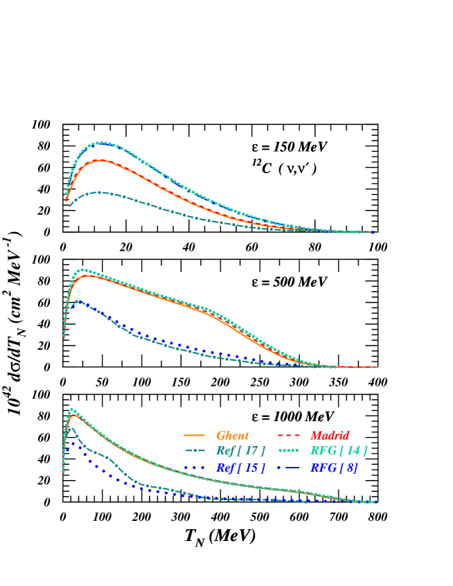
Figure 2: Neutral current ¹²C$({\nu},{\nu}^{\prime})$ cross sections as a function of the outgoing nucleon kinetic energy $T_{N}$ at different incoming neutrino energies. The solid (dashed) lines represent the RPWIA results of the Ghent (Madrid) group. The short-dot-dashed lines show the RPWIA results of Ref. vanderventel04 , and the long-dotted lines those of Ref. meuccineut . The short-dotted (long-dot-dashed) line shows the predictions of the RFG model of Ref. mai (Ref. horo ) with a binding-energy correction of $27$ MeV.

III.1 RPWIA

Fig. 2 shows the results of various RPWIA calculations for ¹²C$(\nu,\nu^{\prime})$ at $150$, $500$ and $1000$ MeV. We observe that the plane-wave limits of our RMSGA and RDWIA formalisms are in excellent agreement. The remaining differences, smaller than 2-3$\%$, can be attributed to the distinctive numerical techniques. This comparison lends us confidence about the consistency of the two types of calculations and the reliability of the adopted numerical techniques.

The fact that our models provide almost identical RPWIA results may seem trivial. As can be appreciated via Fig. 2, however, our RPWIA predictions disagree with the ones of Refs. meuccineut and vanderventel04 . Although the RPWIA calculations of Refs. meuccineut and vanderventel04 are mutually consistent at $\varepsilon=500$ MeV, this is no longer the case at $\varepsilon=1$ GeV. In the search for the origin of the discrepancies between our and other RPWIA calculations, differences in the nuclear current can be ruled out. The current operator of Eq. (41) used along this work is formally identical to the one mentioned in Refs. meuccineut and vanderventel04 , and the same holds for the form-factor parameterization. Only the bound-state wave functions used in Refs. meuccineut and vanderventel04 differ from ours. We have performed cross section calculations with various parameterizations for the bound state wave functions, and found almost negligible differences.

The role of the various terms $F_{1}$, $F_{2}$ and $G_{A}$ in Eq. (41) in the NC differential cross section was investigated in Ref. vanderventel04 . The results were shown for proton knockout from the $1p_{3/2}$ orbital of ¹²C, at incident neutrino energies of 150, 500 and 1000 MeV. In Fig. 3 we analyse the contribution of the $F_{1}$, $F_{2}$ and $G_{A}$ form factors in our cross sections under the same circumstances. First, let us observe that the calculations performed by setting $F_{1}=0$ (long-dot-dashed lines) almost reproduce the full cross sections (solid lines). This shows, in agreement with the outcomes of Ref. vanderventel04 , that the contribution of the Dirac form factor is very small. The cross section can then be very well approximated as a sum of three terms: one proportional to ($G_{A}$)², a second proportional to ($F_{2}$)², and a third proportional to the interference of $G_{A}$ and $F_{2}$ contributions. The term proportional to ($G_{A}$)² (dashed lines) is very similar to the corresponding one in Fig. 11 of Ref. vanderventel04 . The same holds for the cross sections obtained by nullifying $G_{A}$ (short-dot-dashed lines), whose behaviour is almost entirely given by $F_{2}^{2}$ term. Thus, the fact that our curves neglecting the $F_{1}$ contribution differ from those in Ref. vanderventel04 can mainly be attributed to the $G_{A}F_{2}$ interference term. Furthermore, the results seem to differ in the sign of this term. As a matter of fact, changing the sign of the $G_{A}F_{2}$ term in our calculations, the cross sections follow closely the ones of Ref. vanderventel04 . At $500$ and $1000$ MeV the differential cross sections of Ref. vanderventel04 display some oscillations as a function of $T_{N}$. As can be appreciated from Fig. 2 and 3, we find no indications for these oscillations. Recently, the authors of Ref. vanderventel04 have extended their work to calculate CC neutrino cross sections vanderventel05 . We remark that for this type of neutrino reactions the magnitude of the cross sections is in agreement with the RPWIA limit of the models presented here.

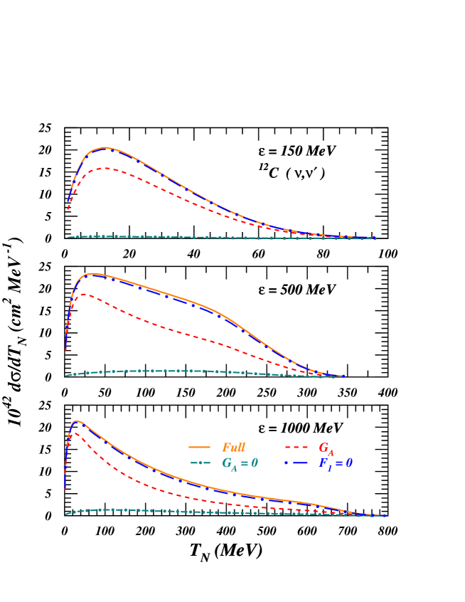
Figure 3: Effect of the different form factors on the neutral current ¹²C$({\nu},{\nu}^{\prime})$ cross sections as a function of $T_{N}$ at different incoming neutrino energies. The solid lines represent the full RPWIA results. The long-dot-dashed (short-dot-dashed) lines show the results with $F_{1}=0$ ($G_{A}=0$). The dashed lines show the cross section when only $G_{A}$ is considered.

It is well known that binding-energy effects tend to vanish with increasing energies. Accordingly, a description of the $\nu$-nucleus scattering process in terms of a RFG model is expected to approach the RPWIA predictions at high incoming neutrino energies. This is observed in Fig. 2, when comparing the RFG results of Refs. horo ; albe1 ; mai with our RPWIA predictions. At $\varepsilon=150$ MeV, our RPWIA cross sections are approximately $15\%$ smaller than the RFG ones. The RFG result from Refs. albe1 ; mai closely follows our RPWIA results at 500 MeV, the agreement at 1 GeV being remarkably good. The observed similarity between the independent RFG predictions of Refs. horo ; albe1 ; mai and our RPWIA results lends us additional confidence that the RPWIA results presented here can serve as benchmark calculations.

III.2 The effect of FSI : RMSGA and RDWIA approaches

Let us now turn our attention to the effect of FSI. NC $\nu$-nucleus cross sections obtained within RDWIA and RMSGA are displayed in Fig. 4. The calculations correspond to ¹²C and ⁵⁶Fe targets, and incoming energies of $500$, $1000$, and $5000$ MeV. Focusing on the results of the RDWIA model, the inclusion of the complex optical potential reduces the RPWIA results by nearly $40-50\%$ for ¹²C. As expected, the global effect of FSI increases with growing atomic number, and reductions of over $60\%$ are obtained for ⁵⁶Fe. The presence of the imaginary term in the optical potential is likely to lead to an underestimation of the single-nucleon knockout contribution to the inclusive cross section. Indeed, in inclusive measurements all possible final channels are included, whilst the RDWIA and RMSGA calculations are confined to ”elastic” single-nucleon knockout.

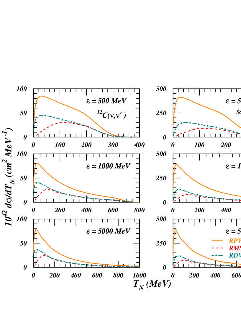
Figure 4: Neutral current ¹²C$({\nu},{\nu}^{\prime})$ (left panels) and ⁵⁶Fe$({\nu},{\nu}^{\prime})$ (right panels) cross sections as a function of $T_{N}$ at different incoming neutrino energies. The solid lines represent the RPWIA predictions of the Madrid group, in agreement with those of the Ghent one. The dashed (dot-dashed) lines implement the effect of FSI within the RMSGA (RDWIA) framework.

Traditionally, Glauber-inspired models have been esteemed to provide reliable results at high energies, as they rely on the eikonal approximation. A very striking outcome of Fig. 4 is that, for integrated quantities as the ones involved in neutrino experiments, the RMSGA cross sections compare very well with the RDWIA ones down to remarkably low ejectile kinetic energies of about $200$ MeV. Below this energy, the RMSGA predictions are not realistic due to the underlying approximations, mainly the postulation of linear trajectories and frozen spectator nucleons.

For the sake of completeness, in Fig. 5 we show our predictions for CC $\nu$-nucleus cross sections. The effects of FSI are of the same order as for NC, and very similar results are also obtained within RMSGA and RDWIA down to very low ejectile kinetic energies.

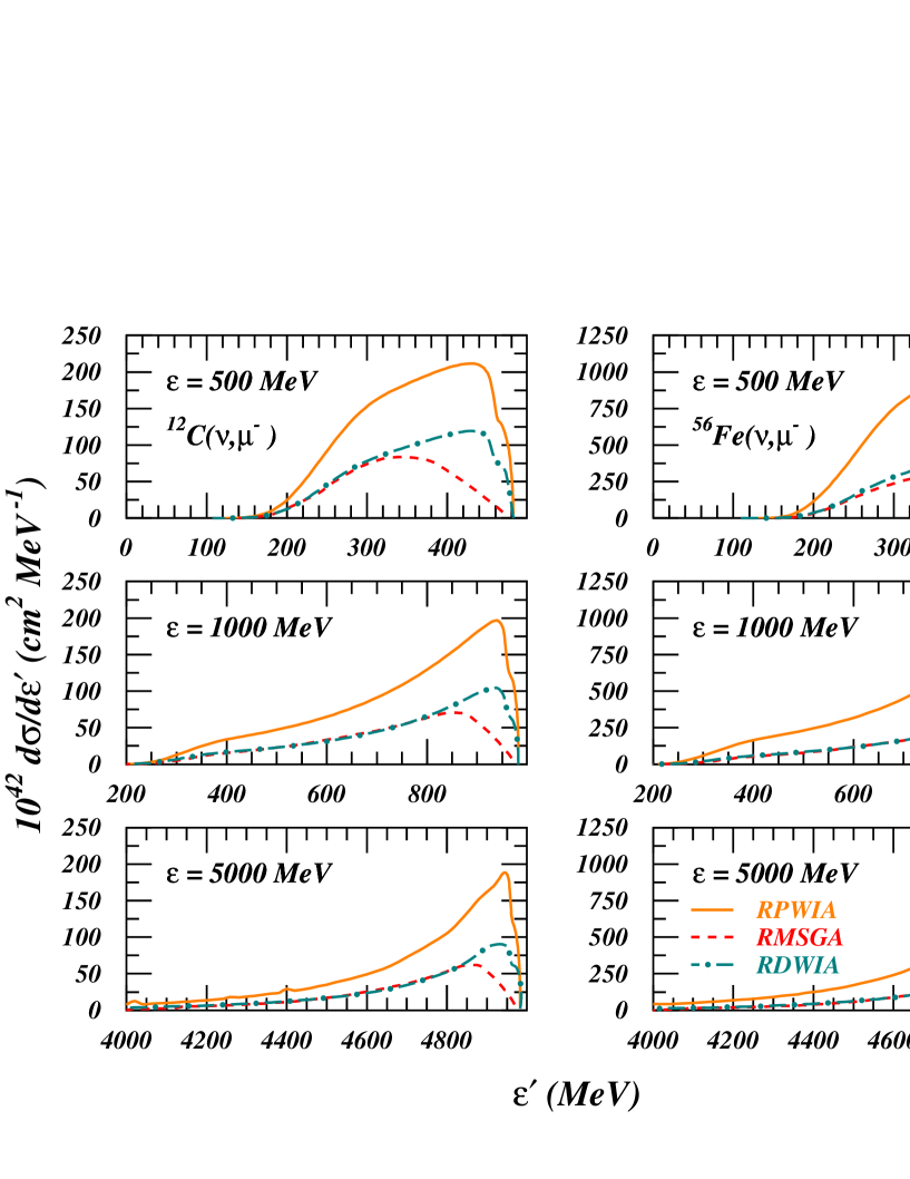
Figure 5: Charged current ¹²C$({\nu}_{\mu},{\mu}^{-})$ (left panels) and ⁵⁶Fe$({\nu}_{\mu},{\mu}^{-})$ (right panels) cross sections as a function of the outgoing lepton energy $\varepsilon^{\prime}$ at different incoming energies. The labeling is the same as in Fig. 4.

III.3 Estimating the effect of FSI mechanisms

A quantity routinely used to estimate the overall effect of FSI in nucleon-emission processes is the nuclear transparency. Intuitively, it provides a measure for the probability that a nucleon of a certain energy - above the particle-emission threshold - can escape from the nucleus without being subject to any further interaction. From this ’definition’, one can expect that the nuclear transparency is identical for neutrino and electron induced nucleon knockout. Once the nucleon is traversing the nuclear medium, only its energy is expected to determine the way it propagates. In addition, neutrinos and electrons can be expected to probe equal amounts of bulk and surface parts of the target nucleus.

Several investigations of the nuclear transparency have been carried out using the $A(e,e^{\prime}p)$ reaction in the QE regime (i.e. the Bjorken variable $x=Q^{2}/(2M_{N}\omega)\approx 1$), and data for different nuclei are now available. The nuclear transparency is extracted from the ratio of the measured $A(e,e^{\prime}p)$ yield to the calculated one using the plane-wave impulse approximation, according to

$$T_{exp}(Q^{2})=\frac{\int_{V}d^{3}p_{m}dE_{m}Y_{exp}(E_{m},\vec{p}_{m},\vec{k}_{f})}{c(A)\int_{V}d^{3}p_{m}dE_{m}Y_{PWIA}(E_{m},\vec{p}_{m})}.$$ (52)

The quantity $V$ specifies the experimental phase-space in missing momentum ($p_{m}$) and energy ($E_{m}$). The kinematics cuts $|p_{m}|\leq 300$ MeV/c and $E_{m}\leq 80$ MeV, in combination with the requirement that $x\approx 1$, guarantee that the electro-induced proton-emission process is predominantly quasi-elastic. The factor $c(A)$ is introduced to correct in a phenomenological way for short-range mechanisms, and is assumed to be moderately target-mass dependent ($c=0.9$ for ¹²C, and $c=0.82$ for ⁵⁶Fe). It accounts for the fact that short-range correlations move a fraction of the single-particle strength to higher missing energies and momenta and, hence, beyond the ranges covered in the integrations of Eq. (52). Without going into details, theoretical predictions are obtained in a similar way from the ratio of distorted-wave calculations to plane-wave ones. In Fig. 6, the transparencies predicted by the RMSGA and the RDWIA models are displayed as a function of $Q^{2}$ for ¹²C and ⁵⁶Fe, together with the world data extracted from $A(e,e^{\prime}p)$. Solid (dot-dashed) lines show the $A(e,e^{\prime}p)$ results within RMSGA (RDWIA). Details about the calculations can be found in Ref. lava04 . The dashed (RMSGA) and dotted (RDWIA) curves correspond to the computed $A(\nu,\nu^{\prime}p)$ transparencies, obtained using the same procedure as for electron scattering. This procedure includes the computation of RDWIA and RPWIA cross sections at $x\approx 1$, averaged over the same phase space used in Eq. (52). As can be seen, within each model the neutrino transparencies agree quite well with their electron counterparts. This result clearly illustrates the fact that in our models the average attenuation effect of the nuclear medium on the emerging nucleon is rather independent of the nature of the leptonic probe.

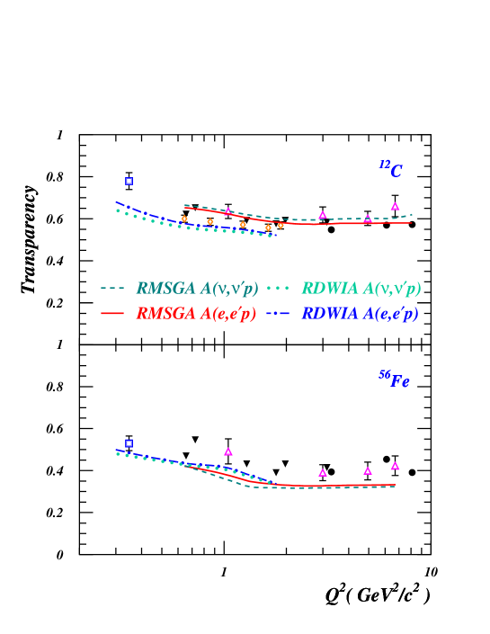
Figure 6: Nuclear transparencies versus $Q^{2}$ for different nuclei in quasi-elastic kinematics. The solid (dot-dashed) lines shows the results of a RMSGA (RDWIA) $A(e,e^{\prime}p)$ calculation lava04 . The dashed (dotted) lines represent the results for $A(\nu,\nu^{\prime}p)$ within RMSGA (RDWIA). Data points are from Refs. Garino92 (open squares), oneill95 ; makins94 (open triangles), Garrow2002 (solid circles), Abbott98 ; Dutta2003 (solid triangles), and rohe05 (diamonds).

Adopting the idea that the nuclear transparency for electrons equals the one for neutrinos, the information obtained about nucleon propagation via $A(e,e^{\prime}p)$ can be used to predict the effects of FSI mechanisms in inclusive QE $\nu$-nucleus cross sections. As the transparency is essentially the ratio of cross sections including FSI to the ones in the plane-wave limit, this will be done by multiplying the RPWIA results for neutrino-nucleus cross sections with the measured transparency factors extracted from $A(e,e^{\prime}p)$. In this scenario, the benchmark RPWIA neutrino-nucleus cross sections are crucial. It is important to realize that we use transparency factors that are confined to $x\approx 1$, while the computation of the inclusive neutrino-nucleus cross section include the full phase-space.

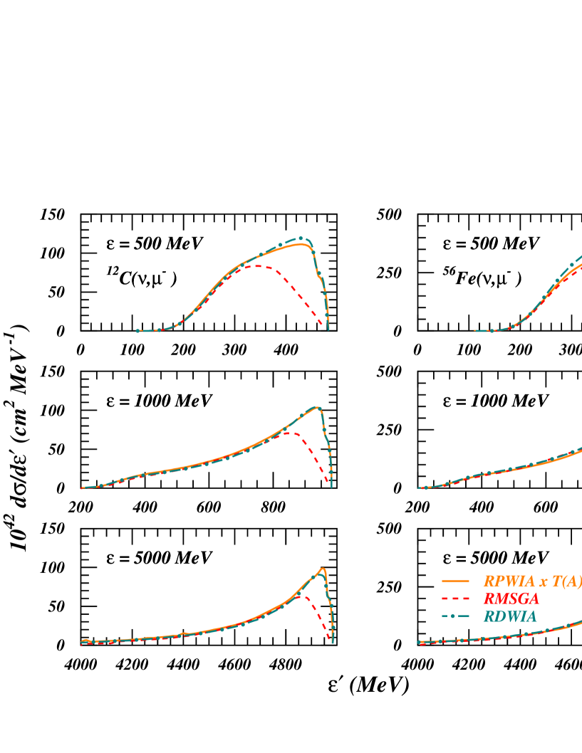
Figure 7: Charged current ¹²C$({\nu}_{\mu},{\mu}^{-})$ (left panels) and ⁵⁶Fe$({\nu}_{\mu},{\mu}^{-})$ (right panels) cross sections as a function of $\varepsilon^{\prime}$ at different incoming energies. The dashed (dot-dashed) lines represent the RMSGA (RDWIA) prediction. The solid lines show the RPWIA results, scaled with a transparency factor $T(^{12}C)\approx 0.52$ and $T(^{56}Fe)\approx 0.34$.

In Fig. 7, the dashed and dot-dashed lines represent the inclusive CC $\nu$-nucleus cross section within RMSGA and RDWIA, respectively. The solid curve displays our corresponding RPWIA calculation, scaled with a constant factor taken as a representative value for the experimental $A(e,e^{\prime}p)$ transparency for the nucleus. For ¹²C (⁵⁶Fe) we take $T\approx 0.52$ ($\approx 0.34$). In extracting these values, we have corrected the measured transparencies from Fig. 6 with the factor $c(A)$. A very good agreement is observed between the rescaled RPWIA and the full RDWIA/RMSGA curves in the case of ¹²C. This finding supports the idea that a simple scaling of the RPWIA results with a transparency factor obtained from electron scattering data allows one to reliably estimate the FSI effects for the quasi-elastic contribution to the inclusive neutrino cross section. The fact that for ⁵⁶Fe the agreement is less satisfactory reflects the fact that our models slightly underestimate the ⁵⁶Fe transparency data.

Finally, Fig. 8 displays the total cross section ($\sigma=\int d\varepsilon^{\prime}(d\sigma/d\varepsilon^{\prime})$) for ¹²C$(\nu_{\mu},\mu^{-})$ and ⁵⁶Fe$(\nu_{\mu},\mu^{-})$ reactions, scaled with the number of neutrons in the target. Results are shown within RPWIA and RDWIA using a complex optical potential. The figure clearly shows that the difference between RPWIA and RDWIA cross sections is approximately given by the experimental transparency factor extracted from $A(e,e^{\prime}p)$ at QE kinematics. Furthermore, other important features can be extracted from this figure. First, the RPWIA cross sections scale with the target mass-number. In this way, when RPWIA cross sections are required for a heavy nucleus, a very good approximation consists in multiplying this cross section per nucleon by its mass number. Second, the cross sections do not appreciably change from neutrino energies above 2 GeV, i.e. the cross sections saturate at high incoming neutrino energies. To finish with, we compare our relativistic calculations with data from various experiments. The RPWIA calculations give a fair account of the neutrino-energy and magnitude of the data. The RPWIA is confined to single-nucleon knockout thereby not including final-state interaction effects. The RDWIA calculations, on the other hand, including FSI effects via the introduction of an optical potential, considerably underestimate the data. The results contained in Fig. 8 indicate that at least $50\%$ of the measured $(\nu_{\mu},\mu^{-})$ strength can be attributed to single-step (”elastic”) nucleon knockout to missing energies below 80 MeV in the residual A-1 nucleus. The remaining fraction of about $50\%$ could be attributed to multi-nucleon knockout, pion production with subsequent reabsorption, single-nucleon knockout to more complex states, … . Adding all these contributions would move the calculations closer to the data.

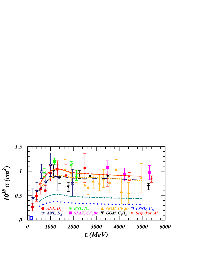
Figure 8: Total CC $(\nu_{\mu},\mu^{-})$ neutrino cross sections as a function of the incoming neutrino energy. The solid (dashed) line shows the RPWIA calculations on ¹²C (⁵⁶Fe). The dot-dashed (long-dotted) curves implement the effect of FSI on ¹²C (⁵⁶Fe) within RDWIA. The short-dotted (long-dashed) show the RMF curve for ¹²C (⁵⁶Fe). All results are scaled with the number of neutrons in the target. Data points are from Refs. barish ; baker ; mann ; brunner ; pohl ; auerbach ; belikov ; bonetti .

It has been suggested serot86 ; kim3 ; caballero05 that the importance of these missing channels can be estimated in a model in which both the single-particle bound-states and scattering states are computed in a real mean-field potential obtained in the Hartree approximation to the $\sigma-\omega$ model. Such an extreme mean-field model (here coined as RMF) involves no imaginary potential and accordingly the loss of single-nucleon knockout strength into ”inelastic” nucleon-knockout channels is effectively reintroduced. As can be appreciated from Fig. 8, the presence of a real potential reduces the RPWIA single-nucleon knockout strength, but the global reduction with respect to RPWIA is much smaller compared to the $50-60\%$ in the RDWIA/RMSGA frameworks. It is remarkable that the energy dependence of the cross section is identical in all three relativistic frameworks adopted here. The magnitude, on the other hand, depends strongly on the model used to account for FSI mechanisms. This reinforces our suggestion that one could use RPWIA results to predict the ”elastic” single-nucleon knockout contribution to inclusive neutrino cross sections, provided that they are rescaled with a transparency factor extracted from $A(e,e^{\prime}p)$ data.

IV Conclusions

We have employed two relativistic models, RMSGA and RDWIA, to study NC and CC quasi-elastic neutrino-nucleus scattering. Results have been presented for carbon and iron targets, covering a wide range of neutrino energies. Within RPWIA both models provide nearly identical results, which deviate from existing RPWIA predictions. The fact that two independently developed codes that adopt very different numerical techniques agree in this limit, together with the fact that our RPWIA predictions approach the RFG model at high energies, give us confidence that our RPWIA calculations serve as benchmark results. We subsequently computed the effects of FSI mechanisms within the RMSGA and RDWIA models. The two ways of dealing with FSI are consistent down to remarkably low outgoing nucleon kinetic energies of about 200 MeV. FSI produce a large reduction of the cross sections, that increases with the mass number of the target nucleus. Finally, we have illustrated that the nuclear transparencies extracted from $A(e,e^{\prime}p)$ measurements can be used to estimate the effect of FSI mechanisms on the elastic single-nucleon knockout contribution to the inclusive neutrino-nucleus cross sections. Extensions of our models include the implementation of pion production and delta resonance. Work in this direction is in progress.

References

- (1) Y. Fukuda et al. (Super-Kamiokande Collaboration), Phys. Rev. Lett. 81, 1562 (1998); M.H. Ahn et al. (K2K Collaboration), Phys. Rev. Lett. 90, 041801 (2003); Q.-R. Ahmad et al. (SNO Collaboration), Phys. Rev. Lett. 87, 071301 (2001) and Phys. Rev. Lett. 89, 011301 (2002); K. Eguchi et al. (KamLAND Collaboration), Phys. Rev. Lett. 90, 021802 (2003); C. Athanassopoulos et al. (LSND Collaboration), Phys. Rev. Lett. 77, 3082 (1996) and Phys. Rev. Lett. 81, 1774 (1998).
- (2) Stuart J. Freedman and Boris Kayser, physics/0411216.
- (3) Minera Collaboration home page http://minerva.fnal.gov/
- (4) John N. Bahcall, Aldo M. Serenelli and Sarbani Basu, Astrophys. J. 621, L85 (2005); John N. Bahcall, hep-ph/0412068
- (5) A. Aprahamian, K. Langanke and M. Wiescher, Prog. Part. Nucl. Phys. 54, 535 (2005)
- (6) Boone home page http://www-boone.fnal.gov/
- (7) NuTeV home page http://www-e815.fnal.gov/NuTeV.html
- (8) C.J. Horowitz, H. Kim, P.D. Murdock, and S. Pollock, Phys. Rev. C 48, 3078 (1993).
- (9) Y. Umino, J.M. Udias, Phys. Rev. C 52, 3399 (1995); Y. Umino, J.M. Udias, P.J. Mulders, Phys. Rev. Lett. 74, 4993 (1995).
- (10) N. Jachowicz, K. Vantournhout, J. Ryckebusch, and K. Heyde, Phys. Rev. Lett. 93, 082501 (2004).
- (11) M.B. Barbaro, A. De pace, T.W. Donnelly, A. Molinari, and M.J. Musolf, Phys. Rev. C 54, 1954 (1996).
- (12) W.M. Alberico, M.B. Barbaro, S.M. Bilenky, J.A. Caballero, C. Giunti, et al., Nucl. Phys. A623, 471 (1997).
- (13) W.M. Alberico, M.B. Barbaro, S.M. Bilenky, J.A. Caballero, C. Giunti, et al., Phys. Lett. B 438, 9 (1998).
- (14) C. Maieron, M.C. Martínez, J.A. Caballero, and J.M. Udías, Phys. Rev. C 68, 048501 (2003).
- (15) A. Meucci, C. Giusti, and F.D. Pacati, Nucl. Phys. A744, 307 (2004).
- (16) A. Meucci, C. Giusti, and F.D. Pacati, Nucl. Phys. A739, 277 (2004).
- (17) B.I.S. van der Ventel and J. Piekarewicz, Phys. Rev. C 69, 035501 (2004).
- (18) C. Bleve, G. Co, I. De Mitri, P. Bernardini, G. Mancarella, D. Martello and A. Surdo, Astropart. Phys. 16, 145 (2001).
- (19) H. Kim, J. Piekarewicz, and C.J. Horowitz, Phys. Rev. C 51, 2739 (1995).
- (20) H. Kim, S. Schramm, and C.J. Horowitz, Phys. Rev. C 53, 2468 (1996);53, 3131 (1996).
- (21) J. Nieves, J.E. Amaro, and M. Valverde, Phys. Rev. C 70, 055503 (2004).
- (22) J.E. Amaro, M.B. Barbaro, J.A. Caballero, T.W. Donnelly, A. Molinari, and I. Sick, Phys. Rev. C 71, 015501 (2005).
- (23) Finesse home page http://www-finesse.fnal.gov/
- (24) J.M Udías, P. Sarriguren, E. Moya de Guerra, E. Garrido and J.A. Caballero, Phys. Rev. C 48, 2731 (1993).
- (25) J.M. Udías, P. Sarriguren, E. Moya de Guerra and J.A. Caballero, Phys. Rev. C 53, R1488 (1996).
- (26) J.M. Udías, J.A. Caballero, E. Moya de Guerra, J.E. Amaro and T.W. Donnelly, Phys. Rev. Lett. 83, 5451 (1999).
- (27) J.M. Udías, J.A. Caballero, E. Moya de Guerra, J.R. Vignote and A. Escuderos, Phys. Rev. C 64, 024614 (2001).
- (28) M.C. Martínez, J.R. Vignote, J.A. Caballero, T.W. Donnelly, E. Moya de Guerra and J.M. Udías, Phys. Rev. C 69, 034604 (2004).
- (29) P. Lava, M.C. Martínez, J. Ryckebusch, J.A. Caballero, and J.M. Udías, Phys. Lett. B 595, 177 (2004).
- (30) P. Lava, J. Ryckebusch, B. Van Overmeire and S. Strauch, Phys. Rev. C 71, 014605 (2005)
- (31) J. Bjorken, and S. Drell, Relativistic Quantum Mechanics,Mc-Graw-Hill, New York, 1964.
- (32) J. Ryckebusch, D. Debruyne, P. Lava, S. Janssen, B. Van Overmeire, and T. Van Cauteren, Nucl. Phys. A 728, 226 (2003).
- (33) B. Serot, and J. Walecka, Adv. Nucl. Phys. 16, 1 (1986).
- (34) T. Donnelly, and A. Raskin, Ann. Phys. 169, 247 (1986).
- (35) R. Furnstahl et al., Nucl. Phys. A615, 441 (1997).
- (36) S. Eidelman et al., Phys. Lett. B 592, 1 (2004), http://pdg.lbl.gov/
- (37) R. Glauber and G. Matthiae, Nucl. Phys. B21, 135 (1970).
- (38) E. D. Cooper, S. Hama, B.C. Clark, and R.L. Mercer, Phys. Rev. C 47, 297 (1993).
- (39) O. Lalakulich and E.A. Paschos, Phys. Rev. D 71, 074003 (2005).
- (40) L.A. Ahrens et al., Phys. Rev. D 35, 785 (1987).
- (41) B.I.S. van der Ventel and J. Piekarewicz, nucl-th/0506071.
- (42) K.S. Kim, L.E. Wright, Yanhe Jin, and D.W. Kosik, Phys. Rev. C 54, 2515 (1996).
- (43) J.A. Caballero, J.E. Amaro, M.B. Barbaro, T.W. Donnelly, C. Maieron, J.M Udías, Phys. Rev. Lett. 95, 252502 (2005).
- (44) G. Garino et al., Phys. Rev. C 45, 780 (1992).
- (45) T. O’Neill et al., Phys. Lett. B 351, 87 (1995).
- (46) N. Makins et al., Phys. Rev. Lett. 72, 1986 (1994).
- (47) K. Garrow et al., Phys. Rev. C 66, 044613 (2002).
- (48) D. Abbott et al., Phys. Rev. Lett. 80, 5072 (1998).
- (49) D. Dutta et al., Phys. Rev. C 68, 064603 (2003), and nucl-ex/0303011.
- (50) D. Rohe et al., Phys. Rev. C 72, 054602 (2005).
- (51) S.J. Barish et al., Phys. Rev. D 16, 3103 (1977).
- (52) N.J. Baker et al., Phys. Rev. D 23, 2499 (1981).
- (53) W.A. Mann et al., Phys. Rev. Lett. 31, 844 (1973).
- (54) J. Brunner et al., Z. Phys. C 45, 551 (1990).
- (55) M. Pohl et al., Lett. Nuovo Cim. 26, 332 (1979).
- (56) L.B. Auerbach et al., Phys. Rev. C 66, 015501 (2002).
- (57) S.V. Belikov et al., Z. Phys. A 320, 625 (1985).
- (58) S. Bonetti et al., Nuovo Cimento A 38, 260 (1977).