Many Body Methods and Effective Field Theory

Abstract

In the framework of pionless nucleon-nucleon effective field theory we study different approximation schemes for the nuclear many body problem. We consider, in particular, ladder diagrams constructed from particle-particle, hole-hole, and particle-hole pairs. We focus on the problem of finding a suitable starting point for perturbative calculations near the unitary limit $(k_{F}a)\to\infty$ and $(k_{F}r)\to 0$, where $k_{F}$ is the Fermi momentum, $a$ is the scattering length and $r$ is the effective range. We try to clarify the relationship between different classes of diagrams and the large $g$ and large $D$ approximations, where $g$ is the fermion degeneracy and $D$ is the number of space-time dimensions. In the large $D$ limit we find that the energy per particle in the strongly interacting system is 1/2 the result for free fermions.

I Introduction

The nuclear many-body problem is of fundamental importance to nuclear physics Bethe:1971 . The traditional approach to the many-body problem is based on the assumption that nucleons can be treated as non-relativistic point-particles interacting mainly via two-body potentials. Three-body potentials, relativistic effects, and non-nucleonic degrees of freedom are assumed to give small corrections. The many-body Schrödinger equation is solved using a variety of methods that involve both variational and numerical aspects.

Over the last several years an alternative approach to nuclear physics based on effective field theory (EFT) methods has been applied successfully to the two and three-nucleon systems Weinberg:1990rz ; Beane:2000fx ; Bedaque:2002mn ; Epelbaum:1999dj . EFT methods have the advantage of being directly connected to QCD, and of providing a framework which is amendable to systematic improvements. The application of EFT to nuclear systems is complicated by the appearance of anomalously small energy scales. In the two-body system these small scales are reflected by the large neutron-neutron and neutron-proton scattering lengths, $a_{nn}(^{1}S_{0})\simeq-18$ fm and $a_{np}(^{3}S_{1})\simeq 5$ fm, respectively. Effective field theories capable of describing systems with anomalously large scattering lengths require summing an infinite number of Feynman diagrams at leading order Weinberg:1990rz .

In this work we wish to study the EFT approach to the nuclear many body problem Hammer:2000xg ; Steele:2000qt ; Kaiser:2001jx ; Furnstahl:2002gt ; Krippa:2002ht ; Lee:2004si ; Koch:1987me . We will focus on the equation of state of pure neutron matter at low to moderate density, a problem that is of relevance to the structure of neutron stars. The neutron matter problem has the theoretical advantage that there are no three-body forces at leading order. As in the two-body system the main obstacle is the large scattering length. If the scattering length was small the equation of state and other quantities of interest could be expanded in $(k_{F}a)$, where $k_{F}$ is the Fermi momentum. This is the standard low density expansion for a hard sphere Fermi gas which was studied by Huang, Lee and Yang in the 1950’s and rederived in the EFT context by Hammer and Furnstahl Huang:1957 ; Lee:1957 ; Hammer:2000xg . In real nuclear matter, however, $|k_{F}a|\gg 1$ and the perturbative low density expansion is not useful.

An interesting system that illustrates the difficulties of the nuclear matter problem is a dilute liquid of non-relativistic spin 1/2 fermions interacting via a short range potential with infinite scattering length. In this case the parameters that characterize the many body problem are either infinite or zero, $|k_{F}a|\to\infty$ and $|k_{F}r|\to 0$, where $a,r$ are the scattering length and the effective range. Dimensional analysis implies that the equation of state is of the form

$$\frac{E}{A}=\xi\frac{3}{5}\frac{k_{F}^{2}}{2m},$$ (1)

where $\xi$ is dimensionless number. For free fermions $\xi=1$, but for strongly correlated fermions the theory contains no obvious expansion parameter and the determination of $\xi$ is a difficult non-perturbative problem. Recent interest in this problem has been fueled by experimental advances in creating cold, dilute gases of fermionic atoms tuned to be near a Feshbach resonance cold . These experiments are beginning to yield results for the equation of state of non-relativistic fermions in the limit $|k_{F}a|\to\infty$.

A plausible strategy for investigating neutron matter is to start from a numerical or variational solution of the “unitary limit” system and to include corrections due to the finite effective range, explicit pion degrees of freedom, many body forces, etc. perturbatively. Recent numerical studies of many body systems with a large scattering length can be found in Carlson:2003wm ; Chen:2003vy ; Wingate:2004wm ; Lee:2004qd . In this work we study analytic many body approximations that could be used as the starting point for a theory of neutron matter based on EFT interactions. We focus on ladder diagrams built from particle-particle or particle-hole bubbles and study whether these approximations can be consistently renormalized and yield a stable $|k_{F}a|\to\infty$ limit. We also examine the relationship of these approaches to the large $g$ and large $D$ limits, where $g$ is the number of fermion fields and $D$ is the number of space-time dimensions.

II Particle-particle ladder diagrams

We will consider non-relativistic fermions governed by an effective lagrangian of the form

$${\cal L}_{\rm eff}=N^{\dagger}\left(i\partial_{0}+\frac{\nabla^{2}}{2M}\right)N-\frac{C_{0}}{2}(N^{\dagger}N)^{2}+\frac{C_{2}}{16}\left[(NN)^{\dagger}(N{\stackrel{{\scriptstyle\leftrightarrow}}{{\nabla}}}^{2}N)+h.c.\right]+\ldots\,,$$ (2)

where $\stackrel{{\scriptstyle\leftrightarrow}}{{\nabla}}=\stackrel{{\scriptstyle\leftarrow}}{{\nabla}}-\stackrel{{\scriptstyle\rightarrow}}{{\nabla}}$. We have not displayed terms with higher derivatives or more powers of the fermion field, including two-derivative terms that act in the $p$-wave channel. The parameters $C_{0}$ and $C_{2}$ are related to the $s$-wave scattering length and the effective range. In the power divergence subtraction (PDS) scheme the relationship is given by Kaplan:1998we

$$C_{0}=-\frac{4\pi/M}{\mu-1/a}\ ,\qquad C_{2}\,k^{2}=\frac{4\pi/M}{(\mu-1/a)^{2}}\frac{r}{2}\;k^{2},$$ (3)

where $\mu$ is the renormalization scale. The advantage of the PDS scheme is that the $C_{i}$ are of natural size even if the scattering length is large. Dimensional regularization with minimal subtraction gives $C_{0}=(4\pi a)/M$ which is unnatural in the limit $a\to\infty$.

We are interested in the energy density and pressure of a many body system with baryon density $\rho$. At zero temperature the density is related to the Fermi momentum via $\rho=gk_{F}^{3}/(6\pi^{2})$, where $g=2$ is the degeneracy factor. The free propagator is given by

$$G_{0}(k)_{\alpha\beta}=\delta_{\alpha\beta}\left(\frac{\theta(k-k_{F})}{k_{0}-k^{2}/2M+i\epsilon}+\frac{\theta(k_{F}-k)}{k_{0}-k^{2}/2M-i\epsilon}\right)\ ,$$ (4)

and describes two types of excitations, holes with momentum $k<k_{F}$ and particles with $k>k_{F}$. Using this propagator and the vertices from equ. (2) we can compute the energy per particle as a perturbative expansion in $(k_{F}a)$. To order $(k_{F}a)^{2}$ the result is Huang:1957 ; Lee:1957 ; Furnstahl:2002gt

$$\frac{E}{A}=\frac{k_{F}^{2}}{2M}\left[\frac{3}{5}+(g-1)\left(\frac{2}{3\pi}(k_{F}a)+\frac{4}{35\pi^{2}}(11-2\log(2))(k_{F}a)^{2}\right)+O((k_{F}a)^{3})\right].$$ (5)

Effective range corrections appear at $O((k_{F}a)^{2}(k_{F}r))$ and if $g$ is bigger than 2 logarithmic terms appear at $O((k_{F}a)^{4}\log(k_{F}a))$.

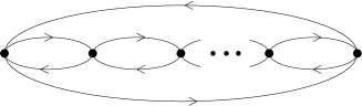
Figure 1: Particle-particle ladder diagrams (left panel) and particle-hole ring diagrams (right panel) in the effective field theory.

This expansion is clearly useless if $(k_{F}a)\gg 1$. In the case of zero baryon density it is well known that an infinite set of bubble diagrams with the leading order contact interaction must be resummed if the two-body scattering length is large. It is natural to extend this calculation to non-zero baryon density by summing particle-particle bubbles with the finite density propagator given in equ. (4). In traditional nuclear physics this approach is known as Brueckner theory Fetter:1971 ; Day:1978 . The elementary particle-particle bubble is given by

$$\int\!\!\frac{d^{3}q}{(2\pi)^{3}}\;\frac{\theta_{q}^{+}}{k^{2}-q^{2}+i\epsilon}=-\frac{\mu}{4\pi}+\frac{k_{F}}{(2\pi)^{2}}f_{PP}(\kappa,s)\ .$$ (6)

We are following here the notation of Steele Steele:2000qt . The theta function $\theta_{q}^{+}\equiv\theta(k_{1}-k_{F})\theta(k_{2}-k_{F})$ with $\vec{k}_{1,2}=\vec{P}/2\pm\vec{k}$ requires both momenta to be above the Fermi surface. The first term on the RHS is the vacuum contribution which contains the PDS renormalization scale $\mu$. The second term is the medium contribution which depends on the scaled relative momentum $\vec{\kappa}=\vec{k}/k_{F}$ and center-of-mass momentum $\vec{s}=\vec{P}/(2k_{F})$. For $s<1$ we have

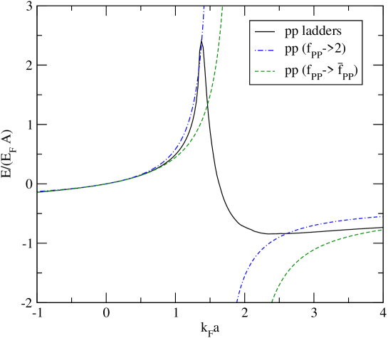
Figure 2: Interaction energy per particle from particle-particle ladder diagrams as a function of $(k_{F}a)$. The curves show a numerical calculation of the ladder sum and the two approximation $f_{PP}\to 2$ and $f_{PP}\to\langle f_{PP}\rangle$ discussed in the text.

$$f_{PP}(\kappa,s)=1+s+\kappa\log\left|\frac{1+s-\kappa}{1+s+\kappa}\right|+\frac{1-\kappa^{2}-s^{2}}{2s}\log\left|\frac{(1+s)^{2}-\kappa^{2}}{1-\kappa^{2}-s^{2}}\right|\ .$$ (7)

Particle-particle ladder diagrams built from the elementary loop integral given in equ. (6) form a geometric series. The contribution of ladder diagrams to the energy per particle is given by Fetter:1971 ; Steele:2000qt

$$\frac{E_{PP}}{A}=\frac{3(g-1)\pi^{2}}{k_{F}^{3}}\int\!\frac{d^{3}P}{(2\pi)^{3}}\frac{d^{3}k}{(2\pi)^{3}}\;\theta_{k}^{-}\;\frac{4\pi a/M}{1-\frac{k_{F}a}{\pi}f_{PP}(\kappa,s)}\ .$$ (8)

This result can be interpreted as the trace of the in-medium particle-particle scattering matrix over all occupied (hole) states. Note that equ. (8) is independent of the renormalization scale parameter $\mu$. This is in contrast to the perturbative result equ. (5) which is independent of $\mu$ only if $a$ is small. In general the integral in equ. (8) has to be performed numerically. Steele suggested that in the large $D$ limit the function $f_{PP}$ can be replaced by its asymptotic value 2 and we will examine this claim in Section V. Another possible approximation is to replace $f_{PP}$ by its phase space average

$$\langle f_{PP}\rangle=\frac{6}{35}\left(11-2\log(2)\right),$$ (9)

where $\langle.\rangle$ denotes an average over all momenta corresponding to occupied (hole) states. In this case we find

$$\frac{E_{PP}}{A}=(g-1)\frac{k_{F}^{2}}{2M}\frac{2(k_{F}a)/(3\pi)}{1-\frac{6}{35\pi}(11-2\log(2))(k_{F}a)}.$$ (10)

This approximation has the virtue that the energy per particle from ladder diagrams agrees with the perturbative result up to $O((k_{F}a)^{2})$. In Fig. 2 we compare the two approximations with numerical results. We observe that all calculations agree fairly well if the scattering length is either negative or positive and large. For $g=2$ the parameter $\xi$ in equ. (1) is given by

$$\xi=0.44\;\;(f_{PP}\to 2),\hskip 14.22636pt\xi=0.32\;\;(f_{PP}\to\langle f_{PP}\rangle),\hskip 14.22636pt\xi=0.24\;\;({\rm num}).$$ (11)

For $g>2$ the results indicate that $\xi$ is negative and the homogeneous low density phase is unstable. The different calculations shown in Fig. 2 disagree strongly in the regime $(k_{F}a)\sim 1$. Approximating $f_{PP}$ by a constant leads to a singularity in the energy per particle. In the numerical calculation this singularity is smoothed out, but a significant enhancement in the energy per particle remains. However, even in this case the particle-particle ladder sum has singularities for certain momenta that correspond to occupied states. These singularities are presumably related to the existence of deeply bound two-body states in the vacuum for $a\sim\mu^{-1}$. In this case interactions between the bound states are essential and the approximations used in this section are not reliable.

III Effective range corrections and hole ladders

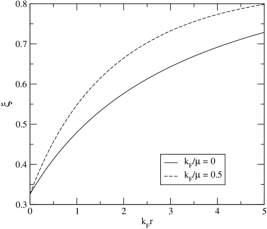
Figure 3: Equation of state of a dilute Fermi gas in the unitary limit $(k_{F}a)\to\infty$ as a function of the effective range. We show the parameter $\xi$ defined in the text as a function of $(k_{F}r)$ for two different values of the Fermi momentum in units of the PDS renormalization scale $\mu$.

In this section we study the question whether the ladder sum can be systematically improved by including higher order terms in the effective lagrangian. The two-derivative term proportional to $C_{2}$ incorporates effective range corrections. At zero baryon density the particle-particle scattering amplitude is Kaplan:1998we

$$T(k)=\frac{C_{0}+C_{2}k^{2}}{1-\frac{M}{4\pi}(\mu+ik)(C_{0}+C_{2}k^{2})}.$$ (12)

The effective range approximation corresponds to keeping $C_{0}$ to all orders but treating $C_{2}$ as a perturbation. The structure of equ. (12) is very simple because in dimensional regularization, in both the MS and PDS renormalization schemes, powers of momentum internal to the elementary particle-particle loop diagrams are converted into powers of the external momentum. At finite density the integrals are more complicated. We discuss the calculation of the bubble sum in the appendix and only present the results here. The energy per particle is

$$\frac{E_{PP}}{A} = \frac{3(g-1)\pi^{2}}{k_{F}^{3}}\int\!\frac{d^{3}P}{(2\pi)^{3}}\frac{d^{3}k}{(2\pi)^{3}}\;\theta_{k}^{-}\frac{1}{1-MC_{0}I_{0}}$$ (13)

$$\hskip 8.5359pt\times\Bigg{\{}C_{0}+C_{2}\frac{(k^{2}+MC_{0}g_{2})(4-MC_{2}g_{2})+MC_{2}g_{4}}{(2-MC_{2}g_{2})^{2}-(4C_{0}+4C_{2}k^{2}-C_{2}^{2}M(k^{2}g_{2}-g_{4}))MI_{0}}\Bigg{\}},$$

where $I_{n}$ and $g_{n}$ are

$$I_{n}(k_{F},\kappa,s) = \int\!\!\frac{d^{3}q}{(2\pi)^{3}}\;\frac{q^{n}\theta_{q}^{+}}{k^{2}-q^{2}+i\epsilon},$$ (14)

$$-g_{n}(k_{F},s) = \int\!\!\frac{d^{3}q}{(2\pi)^{3}}\;q^{n-2}\theta_{q}^{+},$$ (15)

and satisfy the following relations

$$I_{0}(k_{F},\kappa,s) = -\frac{\mu}{4\pi}+\frac{k_{F}}{(2\pi)^{2}}f_{PP}(\kappa,s),$$ (16)

$$I_{2}(k_{F},\kappa,s) = k^{2}I_{0}(k_{F},\kappa,s)+g_{2}(k_{F},s),$$ (17)

$$I_{4}(k_{F},\kappa,s) = k^{2}I_{2}(k_{F},\kappa,s)+g_{4}(k_{F},s).$$ (18)

The explicit forms of $g_{2}$ and $g_{4}$ are

$$g_{2} \equiv \frac{k_{F}^{3}}{\pi^{2}}\bar{g}_{2}(s)=\frac{k_{F}^{3}}{\pi^{2}}\left[-\frac{1}{3}+\theta(1-s)\left(\frac{1}{6}-\frac{s}{4}+\frac{s^{3}}{12}\right)\right],$$ (19)

$$g_{4} \equiv \frac{k_{F}^{5}}{\pi^{2}}\bar{g}_{4}(s)=\frac{k_{F}^{5}}{\pi^{2}}\left[-\frac{1}{5}-\frac{s^{2}}{3}+\theta(1-s)(1-s)^{3}\left(\frac{1}{10}+\frac{s}{20}+\frac{s^{2}}{60}\right)\right],$$ (20)

and both $g_{2}$ and $g_{4}$ vanish as $k_{F}\to 0$. If $k_{F}^{2}C_{2}\ll C_{0}$ then equ. (13) can be simplified to

$$\frac{E_{PP}}{A}=\frac{3(g-1)\pi^{2}}{k_{F}^{3}}\int\!\frac{d^{3}P}{(2\pi)^{3}}\frac{d^{3}k}{(2\pi)^{3}}\;\theta_{k}^{-}\frac{1}{1-C_{0}MI_{0}}\left\{C_{0}+C_{2}\frac{k^{2}+MC_{0}g_{2}}{1-C_{0}MI_{0}}\right\}$$ (21)

Using equ. (3) to relate the coupling constants $C_{0}$ and $C_{2}$ to the scattering length and the effective range we find

$$\frac{E_{PP}}{A} = \frac{3(g-1)\pi^{2}}{k_{F}^{3}}\int\!\frac{d^{3}P}{(2\pi)^{3}}\frac{d^{3}k}{(2\pi)^{3}}\;\theta_{k}^{-}\;\frac{4\pi a/M}{1-\frac{k_{F}a}{\pi}f_{PP}(\kappa,s)}$$ (22)

$$\;\times\left\{1+\frac{(k_{F}a)(k_{F}r)}{1-\frac{k_{F}a}{\pi}f_{PP}(\kappa,s)}\left[\frac{\kappa^{2}}{2}+\frac{k_{F}a}{(k_{F}a)(\mu/k_{F})-1}\cdot\frac{2\bar{g}_{2}}{\pi}\right]\right\}.$$

We observe that the energy per particle depends on the renormalization scale $\mu$. We are particularly interested in the situation when $|k_{F}a|\gg 1$ and $|k_{F}r|<1$ for which

$$\frac{E_{PP}}{A} = \frac{3(g-1)\pi^{2}}{k_{F}^{3}}\int\!\frac{d^{3}P}{(2\pi)^{3}}\frac{d^{3}k}{(2\pi)^{3}}\;\theta_{k}^{-}\;\frac{4\pi a/M}{1-\frac{k_{F}a}{\pi}f_{PP}(\kappa,s)}$$ (23)

$$\times\left\{1+\frac{(k_{F}a)(k_{F}r)}{1-\frac{k_{F}a}{\pi}f_{PP}(\kappa,s)}\left[\frac{\kappa^{2}}{2}+\frac{k_{F}}{\mu}\cdot\frac{2\bar{g}_{2}}{\pi}\right]\right\}.$$

We find that effective range corrections are small and independent of $\mu$ provided $|k_{F}r|<1$ and $k_{F}/\mu<1$. Evaluating the integral by replacing $f_{PP}$ and $g_{2}$ by their phase space averages and taking $k_{F}a\to\infty$ we get

$$\xi(k_{F}r)=0.32+0.19(k_{F}r)+O(k_{F}/\mu,(k_{F}r)^{2}).$$ (24)

Using equ. (13) we can also study the behavior of the universal parameter $\xi$ for larger values of $k_{F}r$. The result is shown in Fig. 3. We observe that the dependence of $\xi$ on $k_{F}r$ becomes weaker as $k_{F}r$ grows. In the limit $k_{F}r\to\infty$ the parameter $\xi$ slowly approaches the free Fermi gas value $\xi=1$ Schwenk:2005ka .

Figure 4: Energy per particle from hole-hole ladder diagrams as a function of $\bar{C}_{0}=Mk_{F}C_{0}/(4\pi)$. $\bar{C}_{0}$ is equal to $(k_{F}a)$ in the $\overline{MS}$ scheme, but in the PDS scheme the relation between $\bar{C}_{0}$ and $(k_{F}a)$ depends on the renormalization scale $\mu$. We also show the perturbative result up to order $\bar{C}_{0}^{2}$.

In addition to higher order corrections to the effective interaction we also consider larger classes of diagrams. A simple extension of the calculation of the particle-particle ladder sum is the inclusion of hole-hole ladders. Following the steps that lead to equ. (8) we find

$$\frac{E_{HH}}{A}=\frac{3(g-1)\pi^{2}}{k_{F}^{3}}\int\!\frac{d^{3}P}{(2\pi)^{3}}\frac{d^{3}k}{(2\pi)^{3}}\;\theta_{k}^{+}\left\{\frac{C_{0}}{1-\frac{k_{F}MC_{0}}{4\pi^{2}}f_{HH}(\kappa,s)}-C_{0}-\frac{k_{F}MC_{0}^{2}}{4\pi^{2}}f_{HH}(\kappa,s)\right\},$$ (25)

where $f_{HH}(\kappa,s)=f_{PP}(\kappa,-s)$ is the hole-hole bubble. We have subtracted the first two terms in the expansion of the geometric series. These terms have UV divergences and need to be treated separately. In our case this is not necessary since the two contributions are already included in the particle-particle ladder sum. We observe that the remaining part of the hole ladders is finite and only depends on $C_{0}$ and not the PDS renormalization scale $\mu$. This implies that if the coupling constant is related to the scattering length according to equ. (3), the energy per particle will depend on the renormalization scale $\mu$. Numerical results for the hole-ladders are shown in Fig. 4. We observe that if $C_{0}$ is of natural size the energy per particle from hole ladders is indeed very small compared to the contribution from particle ladders.

IV Particle-hole ring diagrams and the large $g$ expansion

Another important class of diagrams is the set of particle-hole ring diagrams. In gauge theories ring diagrams play a crucial role since they incorporate screening corrections and their inclusion of is necessary to achieve a well behaved perturbative expansion. In theories with short range interactions particle-hole bubbles also provide important corrections to the effective interaction. For example, particle-hole screening corrections reduce the s-wave BCS gap by a factor $\sim 1/2$ in the weak coupling limit.

The real and imaginary parts of the particle-hole bubble are given by Fetter:1971

$${\rm Re}\,\Pi_{0}(\nu,q) = \frac{Mk_{F}}{4\pi^{2}}\Bigg{\{}-1+\frac{1}{2q}\bigg{(}1-\bigg{(}\frac{\nu}{q}-\frac{q}{2}\bigg{)}^{2}\bigg{)}\ln\left|\frac{1+(\nu/q-q/2)}{1-(\nu/q-q/2)}\right|$$ (26)

$$\mbox{}\hskip 56.9055pt-\frac{1}{2q}\bigg{(}1-\bigg{(}\frac{\nu}{q}+\frac{q}{2}\bigg{)}^{2}\bigg{)}\ln\left|\frac{1+(\nu/q+q/2)}{1-(\nu/q+q/2)}\right|\Bigg{\}}$$

$${\rm Im}\,\Pi_{0}(\nu,q) = -\frac{Mk_{F}}{8\pi q}\left\{\begin{array}[]{ccc}1-\left(\frac{\nu}{q}-\frac{q}{2}\right)^{2}&q>2,&\frac{q^{2}}{2}+q\geq\nu\geq\frac{q^{2}}{2}-q\,,\\ 1-\left(\frac{\nu}{q}-\frac{q}{2}\right)^{2}&q<2,&q+\frac{q^{2}}{2}\geq\nu\geq q-\frac{q^{2}}{2}\,,\\ 2\nu&q<2,&0\leq\nu\leq q-\frac{q^{2}}{2}\,,\end{array}\right.$$ (30)

where $\nu=k_{0}M/k_{F}^{2}$ and $q=|\vec{k}|/k_{F}$. Ring diagrams containing particle-hole bubbles can be summed in essentially the same way as the particle-particle ladders. The main difference arises from different spin and symmetry factors. The spin factor of the $n$-th order particle-particle ladder contribution is $g(g-1)2^{n}$. The spin factors of particle-hole diagrams are more complicated. The situation simplifies in the limit of large $g$, often called the large $N$ limit, as it is equivalent to the limit of a large number $N$ of degenerate spin 1/2 fermions. In this case every particle-hole bubble contributes a factor $g$. Indeed, one can show that the particle-hole ring diagrams are the leading diagrams in the large $g$ limit Furnstahl:2002gt .

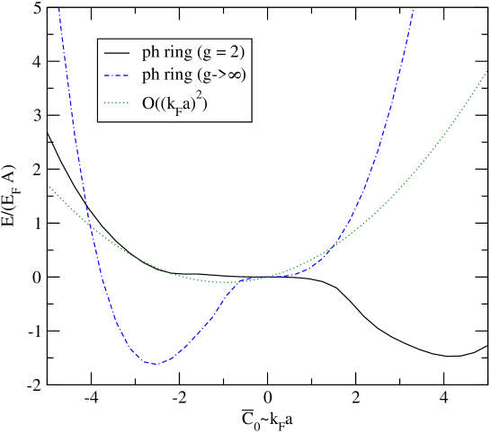
Figure 5: Energy per particle from particle-hole ring diagrams as a function of $\bar{C}_{0}=Mk_{F}C_{0}/(4\pi)$. $\bar{C}_{0}$ is equal to $(k_{F}a)$ in the $\overline{MS}$ scheme, but in the PDS scheme the relation between $\bar{C}_{0}$ and $(k_{F}a)$ depends on the renormalization scale $\mu$. We also show the perturbative result up to order $\bar{C}_{0}^{2}$.

The $n$-th order diagrams in both the particle-particle ladder sum and the particle-hole ring sum have symmetry factors $1/n$. In the case of the ladder diagrams this factor is canceled by a factor $n$ specifying the $n$ different ways in which the diagram can be cut to represent it as a particle-particle Green function integrated over all occupied states. For the ring diagrams it is more convenient to carry out the energy integration explicitly, and no factor $n$ appears. As a consequence, the sum of all ring diagrams is a logarithm. In the large $g$ limit we find

$$E=-\frac{i}{2}\int\frac{d^{4}k}{(2\pi)^{4}}\left[\log\left(1-gC_{0}\Pi(k)\right)+gC_{0}\Pi_{0}(k)+\frac{1}{2}\left(gC_{0}\Pi_{0}(k)\right)^{2}\right],$$ (31)

where we have subtracted the first two terms in the expansion of the logarithm in order to make the integral convergent. These two terms can be computed separately and correspond to the first two terms of the perturbative expansion given in equ. (5). Equ. (31) shows that the correct way to take the large $g$ limit is to keep $gC_{0}$ constant as $g\to\infty$. In this case the free Fermi gas contribution as well as the $O(k_{F}a)$ correction in equ. (5) is of order $O(1)$ while the ring diagrams give a correction of order $O(1/g)$.

Since the energy is real, the integral in equ. (31) can be written as Fetter:1971 ; Furnstahl:2002gt

$$\frac{E}{A} = \frac{3}{g\pi}\left(\frac{k_{F}^{2}}{2M}\right)\int_{0}^{\infty}q^{2}dq\int_{0}^{\infty}d\nu\Bigg{[}gC_{0}\,{\rm Im}\,\Pi_{0}(\nu,q)+(gC_{0})^{2}\,{\rm Im}\,\Pi_{0}(\nu,q){\rm Re}\,\Pi_{0}(\nu,q)$$ (32)

$$\hskip 28.45274pt\mbox{}-\arctan\left(\frac{gC_{0}\,{\rm Im}\,\Pi_{0}(\nu,q)}{gC_{0}{\rm Re}\,\Pi_{0}(\nu,q)-1}\right)\Bigg{]}.$$

In the PDS scheme $C_{0}$ is related to the scattering length by equ. (3) and the ring energy depends of the renormalization scale. Numerical results (for $g=2$) are shown in Fig. 5. For simplicity we have taken $\mu=0$. In this case the energy per particle goes to infinity as $(k_{F}a)\to\infty$. For other values of $\mu$ the energy is finite, but strongly dependent on $\mu$. We also observe that the ring energy per particle is less than $3E_{F}/5$ for $(k_{F}a)<0.9$, which implies an instability of the homogeneous system.

We emphasized above that equ. (31) is correct only in the large $g$ limit. We can also compute the ring sum for $g=2$. In this case there are two possible channels with total spin zero and one. The $n$-th order ring diagram has spin factor $(-2,4,-2,4,\ldots)$. The sum of all ring diagrams is

$$E = -\frac{i}{2}\int\frac{d^{4}k}{(2\pi)^{4}}\Big{[}\log\left(1-C_{0}\Pi(k)\right)+3\log\left(1+C_{0}\Pi(k)\right)$$ (33)

$$\hskip 142.26378pt\mbox{}-2C_{0}\Pi_{0}(k)+2\left(C_{0}\Pi_{0}(k)\right)^{2}\Big{]}.$$

The integral can be calculated as in equ. (32) and the result is shown in Fig. 5. We observe that although the correct $g=2$ result is quite different from the $g\to\infty$ result evaluated at $g=2$, qualitative features, like $E/A\to\infty$ as $C_{0}\to\infty$ and the presence of an unstable regime with $E/A<3E_{F}/5$, remain unchanged.

V Large $D$ expansion

In the previous section we saw that the particle-hole ring energy can be interpreted as the leading order contribution to the energy in the large $g$ limit. This raises the question whether there exists an expansion that gives the ladder sum as the leading order contribution. In a very interesting paper Steele suggested that expansing in $1/D$, where $D$ is the number of space-time dimensions, is the desired scheme Steele:2000qt . If true the $1/D$ expansion offers a systematic approach to the fermion many-body system in the limit $(k_{F}a)\to\infty$.

The main idea is that many body diagrams in a degenerate Fermi system are very sensitive to the available phase space and that the scaling behavior of phase space factors in the large $D$ limit could be a basis for a geometric expansion. Steele argued that the $1/D$ expansion corresponds to the hole-line expansion in traditional nuclear physics, and that it is consistent with EFT power counting for systems with a large scattering length. In this section we shall examine these claims in more detail.

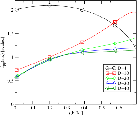
Figure 6: Scaled particle-particle scattering amplitude $Df_{PP}^{(D)}(\kappa,s)$ for $\kappa=s$ (left panel) and $s=0$ (right panel). We observe that except in the BCS limit $s=0,\kappa\to 1$ the function $Df_{PP}^{(D)}$ approaches a smooth limit as $D\to\infty$.

The spatial density of a free Fermi gas in $D$ space-time dimensions is given by

$$\rho=\frac{\Omega_{D-1}}{(2\pi)^{D-1}}\frac{k_{F}^{D-1}}{D-1},\hskip 14.22636pt\Omega_{D-1}=\frac{2\pi^{(D-1)/2}}{\Gamma(\frac{D-1}{2})},$$ (34)

where $\Omega_{D}$ is the surface area of a $D$-dimensional unit ball. In the following we will always take the degeneracy factor $g=2$. The energy per particle is

$$\frac{E_{0}}{A}=\frac{D-1}{D+1}\left(\frac{k_{F}^{2}}{2M}\right)=\left\{1-\frac{2}{D}+\ldots\right\}\left(\frac{k_{F}^{2}}{2M}\right).$$ (35)

We can compute perturbative corrections to this result in $D$ dimensions. To leading order in $C_{0}$ we find

$$\frac{E_{1}}{A}=\frac{1}{D-1}\left[\frac{\Omega_{D-1}C_{0}k_{F}^{D-3}M}{(2\pi)^{D-1}}\right]\left(\frac{k_{F}^{2}}{2M}\right).$$ (36)

This expression indicates that in the weak coupling limit the large $D$ limit should be taken in such a way that

$$\lambda\equiv\left[\frac{\Omega_{D-1}C_{0}k_{F}^{D-3}M}{D(2\pi)^{D-1}}\right]\stackrel{{\scriptstyle D\to\infty}}{{\longrightarrow}}{\it const}.$$ (37)

In the following we wish to study whether this limit is smooth even if the theory is non-perturbative, and what class of diagrams is dominant. For this purpose we consider the in medium particle-particle bubble for an arbitrary number of space-time dimensions $D$. The result is

$$\int\!\!\frac{d^{D-1}q}{(2\pi)^{D-1}}\;\frac{\theta_{q}^{+}}{k^{2}-q^{2}+i\epsilon}=f_{vac}(k)+\frac{k_{F}^{D-3}\Omega_{D-1}}{2(2\pi)^{D-1}}f_{PP}(\kappa,s),$$ (38)

where

$$f_{PP}^{(D)}(\kappa,s)=\frac{2}{c_{D}}\int_{\sqrt{1-s^{2}}}^{1+s}dt\,c\left(D,x_{0}(s,t)\right)\frac{t^{D-2}}{\kappa^{2}-t^{2}}-2I_{2}(D,s,\kappa)$$ (39)

with $x_{0}(s,t)=(s^{2}+t^{2}-1)/(2st)$. The factor 2 was inserted in equ. (39) so that the normalization of $f_{PP}^{(D)}$ is consistent with the previous case $D=4$. The other terms are

$$c(D,x_{0}) = 2x_{0}\;\mbox{}_{2}F_{1}\left(\frac{1}{2},2-\frac{D}{2},\frac{3}{2},x_{0}^{2}\right),$$ (40)

$$c_{D}\equiv c(D,1) = \sqrt{\pi}\frac{\Gamma\left(\frac{D}{2}-1\right)}{\Gamma\left(\frac{D-1}{2}\right)},$$ (41)

$$I_{2}(D,s,\kappa) = \frac{\mbox{}_{2}F_{1}\left(1,\frac{D-1}{2},\frac{D+1}{2},\frac{1+s}{\kappa^{2}}\right)}{(D-1)\kappa^{2}(1+s)^{1-D}},$$ (42)

where $\mbox{}_{2}F_{1}(a,b,c,z)$ is the hypergeometric function. Numerical results for the function $f_{PP}^{(D)}(s,\kappa)$ are shown in Fig. 6. We observe that the particle-particle bubble scales as

$$f_{PP}^{(D)}(s,\kappa)=\frac{1}{D}f_{PP}^{0}(s,\kappa)\left(1+O\left(\frac{1}{D}\right)\right).$$ (43)

The scaling behavior can be verified analytically in certain limits. We find, in particular,

$$f_{PP}^{(D)}(0,0)=\frac{2}{D-3}.$$ (44)

There is a subtlety associated with the BCS singularity at $s=0,\kappa\to 1$. Fig. 6b shows that the logarithmic singularity is not suppressed by $1/D$. We observe, however, that the range of momenta for which $f_{PP}$ is enhanced shrinks to zero as $D\to\infty$. We will study pairing in the large $D$ limit in Sect. VI.

Since $f_{PP}^{(D)}\sim 1/D$ we conclude that if the large $D$ limit is taken according to equ. (37) then all ladder diagrams with particle-particle bubbles are of the same order in $1/D$. The sum of all ladder diagrams can be calculated by noting that, except for the logarithmic (BCS) singularity at $s=0,\kappa=1$, the particle-particle bubble is a smooth function of the kinematic variables $s$ and $\kappa$. Hole-hole phase space, on the other hand, is strongly peaked at $\bar{s}=\bar{\kappa}=1/\sqrt{2}$ in the large $D$ limit. This can be seen by re-expressing $s,\kappa$ in terms of $k_{1,2}$ and using $\bar{k}_{1,2}\to k_{F}$ as $D\to\infty$. If the phase space is strongly peaked we can replace the function $f_{PP}^{(D)}(s,\kappa)$ by its value at $\bar{s},\bar{\kappa}$. We have not been able to calculate the large $D$ limit of $f_{PP}^{(D)}(\bar{s},\bar{\kappa})$ analytically. Our numerical results show that $\lim_{D\to\infty}f_{PP}^{(D)}(\bar{s},\bar{\kappa})/f_{PP}^{(D)}(0,0)=2.02\pm 0.02$. We therefore conjecture that $f_{PP}^{(D)}(\bar{s},\bar{\kappa})=4/D\cdot(1+O(1/D)))$.

We illustrate the method by calculating the second order correction. This contribution involves an integral of the particle-particle bubble over hole-hole phase space. We find

$$\int\frac{d^{D-1}P}{(2\pi)^{D-1}}\int\frac{d^{D-1}k}{(2\pi)^{D-1}}\theta_{k}^{-}f_{PP}^{(D)}(\kappa,s)=\frac{k_{F}^{2D-2}}{D^{2}}\left[\frac{\Omega_{D-1}}{(2\pi)^{D-1}}\right]^{2}\frac{4}{D}\left(1+O\left(\frac{1}{D}\right)\right),$$ (45)

and the energy per particle is given by

$$\frac{E_{2}}{A}=2\left[\frac{\Omega_{D-1}C_{0}k_{F}^{D-3}M}{D(2\pi)^{D-1}}\right]^{2}\left(\frac{k_{F}^{2}}{2M}\right).$$ (46)

Higher order terms can be calculated in the same fashion. As in $D=4$, particle-particle ladder diagrams sum to a geometric series. We get

$$\frac{E}{A}=\left\{1+\frac{\lambda}{1-2\lambda}+O\left(\frac{1}{D}\right)\right\}\left(\frac{k_{F}^{2}}{2M}\right),$$ (47)

where $\lambda$ is the coupling constant defined in equ. (37). We observe that if the strong coupling limit $\lambda\to\infty$ is taken after the limit $D\to\infty$ the universal parameter $\xi$ is given by 1/2.

We have been able to compute the particle ladder contribution to the energy per particle in the large $D$ limit. Steele argued that all other contributions are suppressed by powers of $1/D$ since each additional hole line involves an integral over the Fermi surface of the type shown in equ. (34) which gives a least one power of $1/D$. It is not clear if this argument is entirely correct. We have found, for example, that the main contribution of the particle-particle bubble also scales as $1/D$. We study this problem in more detail in Secs. VI and VII where the potentially relevant pairing and screening corrections are examined, respectively.

VI Pairing in the large $D$ limit

In the previous section we noticed that in the large $D$ limit the particle-particle bubble is enhanced when $s=0$ and $\kappa\to 1$. In this limit the two particles are on opposite sides of the Fermi surface and the logarithmic enhancement of $f_{PP}$ is the well known BCS singularity. The result suggests that in the large $D$ limit the pairing energy might dominate all other contributions to the energy density. In this section we shall study this question by computing the BCS gap and the pairing energy in the large $D$ limit.

If the interaction is weak and attractive we can derive the standard BCS gap equation (see, for example, reference Schafer:2003vz )

$$\Delta=\frac{|C_{0}|}{2}\int\frac{d^{D-1}p}{(2\pi)^{D-1}}\frac{\Delta}{\sqrt{\epsilon_{p}^{2}+\Delta^{2}}}$$ (48)

with $\epsilon_{p}=E_{p}-E_{F}$ and $E_{p}=p^{2}/(2M)$. The integral in equ. (48) can be carried analytically for arbitrary $D$. We find Papenbrock:1998wb ; Marini:1998

$$1=\frac{D\lambda\pi}{\sin(\pi\alpha)}\left(1+x^{2}\right)^{\alpha/2}P_{\alpha}\left(-\frac{1}{\sqrt{1+x^{2}}}\right)$$ (49)

where $\lambda$ is the dimensionless coupling constant defined in equ. (37), $x=\Delta/E_{F}$ is the dimensionless gap, $P_{\alpha}(z)$ is the Legendre function and $\alpha=(D-3)/2$. We note that by going to arbitrary $D$ we have regularized the UV divergence in the gap equation using dimensional regularization. If the gap is small, $x\ll 1$, equ. (49) can be solved using the asymptotic behavior of the Legendre function $P_{\alpha}(z)$ near the logarithmic singularity at $z=-1$ Erdelyi:1953

$$P_{\alpha}(z)\sim\frac{\sin(\alpha\pi)}{\pi}\left(\log\left(\frac{1+z}{2}\right)+2\gamma+2\psi(\alpha+1)+\pi\cot(\alpha\pi)\right).$$ (50)

To leading order in $1/D$ we can also use the asymptotic expression for the Digamma function $\psi(\alpha)=\Gamma^{\prime}(\alpha)/\Gamma(\alpha)\simeq\log(\alpha)+O(1/\alpha)$. We find

$$\Delta=\frac{2e^{-\gamma}E_{F}}{D}\exp\left(-\frac{1}{D\lambda}\right)\left(1+O\left(\frac{1}{D}\right)\right),$$ (51)

where $\gamma\simeq 0.5772$ is Euler’s constant. We observe that the exponential suppression of the gap disappears if the large $D$ limit is taken at fixed $\lambda$. However, the exponential suppression in $\lambda$ is replaced by a power suppression in $1/D$.

Next we calculate the pairing contribution to the energy density. In the weak coupling limit we have Schafer:1999fe

$$E=\int\frac{d^{D-1}p}{(2\pi)^{D-1}}\left\{-\frac{\Delta^{2}}{2\sqrt{\epsilon_{p}^{2}+\Delta^{2}}}+\sqrt{\epsilon_{p}^{2}+\Delta^{2}}-\epsilon_{p}\right\}.$$ (52)

The integrals can be calculated in the same fashion as the integral that appears in the gap equation. We find

$$E = -\frac{\Omega_{D-1}}{(2\pi)^{D-1}}E_{F}k_{F}^{D-1}\frac{\pi}{2}\left(1+x^{2}\right)^{\alpha/2}\left\{\left[\frac{1}{\alpha+2}-\frac{\alpha x^{2}}{2\alpha+4}\right]P_{\alpha}\left(-\frac{1}{\sqrt{1+x^{2}}}\right)\right.$$ (53)

$$\hskip 113.81102pt\mbox{}\left.+\frac{\sqrt{1+x^{2}}}{\alpha+2}P_{\alpha+1}\left(-\frac{1}{\sqrt{1+x^{2}}}\right)\right\}.$$

In the limit $x\to 0$ the logarithmic singularities in the two terms in the curly brackets cancel and the energy per particle is proportional to $x^{2}$. We find

$$\frac{E}{A}=-\frac{D-1}{4}E_{F}\left(\frac{\Delta}{E_{F}}\right)^{2}.$$ (54)

Since $\Delta/E_{F}=O(1/D)$ we conclude that the pairing energy per particle scales as $1/D$ in the large $D$ limit. This implies that the pairing energy is suppressed compared to the contribution from the ladder sum given in equ. (47).

VII Screening in the large $D$ limit

Figure 7: First order screening correction to the effective particle-particle interaction.

In $D=4$ dimensions screening of the elementary four fermion interaction by particle-hole pairs gives an important contribution to the effective interaction. It is well known, for example, that screening reduces the magnitude of the gap in the weak coupling limit by a factor $(4e)^{1/3}\sim 2.2$ Gorkov:1961 . On the other hand, if the $1/D$ expansion corresponds to an expansion in the number of hole lines then we expect that the screening correction should scale as $1/D$ in the large $D$ limit. The basic particle-hole bubble is given by

$$\Pi(\nu,q)=\frac{Mk_{F}^{D-3}\Omega_{D-1}}{(2\pi)^{D-1}}f_{PH}(\nu,q)$$ (55)

with

$$f_{PH}(\nu,q)=\frac{1}{c_{D}}\int_{0}^{1}k^{D-2}dk\int_{-1}^{1}dx(1-x^{2})^{D/2-2}\frac{2\omega_{qk}}{\nu^{2}-\omega_{qk}^{2}},$$ (56)

where $\omega_{qk}=qkx+q^{2}/2$. This integral can be evaluated analytically in $D=4$ and reduces to equ. (26). The particle-hole bubble leads to a renormalization of the effective interaction as shown in Fig. 7. In the weak coupling limit only the interaction of two quasi-particles near the Fermi surface is important. For $s$-wave pairing we can write

$$C_{eff}=C_{0}+C_{0}^{2}\frac{Mk_{F}^{D-3}\Omega_{D-1}}{(2\pi)^{D-1}}\bar{f}_{PH}$$ (57)

where $\bar{f}_{PH}$ is an average over the Fermi surface

$$\bar{f}_{PH}=\frac{1}{c_{D}}\int_{-1}^{1}dx\,(1-x^{2})^{D/2-2}f_{PH}\left(0,\sqrt{2(1-x)}\right).$$ (58)

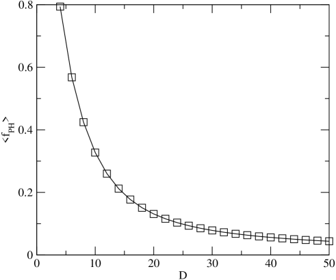
Figure 8: Screening correction to the effective $s$-wave particle-particle interaction as a function of the number of space-time dimensions $D$.

Replacing the bare interaction with the effective one in the BCS gap equation leads to a correction for the pairing gap. We find

$$\Delta=\frac{2e^{-\gamma}E_{F}}{D}\exp\left(-\bar{f}_{PH}\right)\exp\left(-\frac{1}{D\lambda}\right).$$ (59)

For $D=4$ the integral in equ. (58) can also be evaluated analytically, yielding $\bar{f}_{PH}=(2\log(2)+1)/3\simeq 0.79$. Numerical results for $D\geq 4$ are shown in Fig. 8. We observe that the screening correction vanishes as $1/D$ for large $D$.

VIII Conclusions

In this work we considered different many body theories for a system of non-relativistic fermions described by an effective field theory. We are interested, in particular, in a systematic approach to the problem of a dilute liquid of fermions in the limit in which the scattering length is large compared to the inter-particle spacing. This led us to consider the large $g$ and large $D$ expansions.

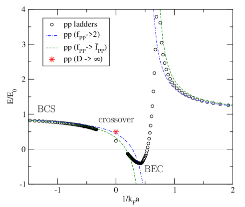
Figure 9: Total energy of an interacting fermion gas in units of the energy of a free fermion gas as a function of $(k_{F}a)^{-1}$. The open circles show the result of a numerical calculation of particle-particle ladder diagrams. The dashed and dash-dotted curves show the two approximations discussed in Sect. II. The star is the result of the $D\to\infty$ calculation in the unitary limit.

At leading order the large $g$ expansion corresponds to summing all particle-hole ring diagrams with the additional approximation that all spin factors are replaced by their large $g$ limits. The problem is that the large $g$ limit is not suitable for studying the limit $|k_{F}a|\to\infty$. Indeed, the naive large $g$ limit corresponds to taking $|k_{F}a|\to 0$. This is also manifest in the functional form of $E/A$ at leading or sub-leading order in $1/g$. The energy per particle in the limit $|k_{F}a|\to\infty$ is strongly dependent on the regularization scale. The only sensible alternative is the Bose limit where we keep $k_{F}a$ fixed and small and take $g\to\infty$ with $\rho=gk_{F}^{3}/(6\pi^{2})$ constant Furnstahl:2002gt ; Jackson:1994 .

From the study of the two-body system in effective field theory we know that if the scattering length is large then the two-body interaction has to summed to all orders. This suggests that a sensible many body theory has to contain at least all particle ladders. We have studied the particle ladder sum in effective field theory. If the particle-particle bubble is replaced by its phase space average then the particle sum can be carried out analytically. This approximation gives $\xi=0.32$ for the universal parameter in the equation of state Heiselberg:2000bm . Numerically, we find a smaller value $\xi\simeq 0.24$. The ladder approximation is unreliable in the regime $(k_{F}a)\sim 1$ in which deeply bound two-body state are important. These results are summarized in Fig. 9. We observe that different approximations agree in the weak coupling (BCS) limit, but give a range of predictions for the crossover behavior.

It is clearly desirable to construct a systematic expansion that contains the ladder sum at leading order. In a very interesting paper Steele suggested that the large $D$ expansion provides the desired approximation scheme. In order to test this idea we have calculated particle ladders for arbitrary $D$. We find that if the coupling constant is scaled appropriately then all particle ladders are indeed of the same order in $1/D$. We also find that the universal parameter $\xi$ is given by $\xi=1/2$, in surprisingly good agreement with the Green function Monte Carlo result $\xi=0.44$ Chang:2004sj . We also verified that the contribution from the pairing energy is suppressed by $1/D$.

There are many questions regarding the $1/D$ expansion that remain to be addressed. We have not been able to construct a general method for computing $1/D$ corrections. We have also not succeeded in showing that the $1/D$ expansion corresponds to an expansion in the number of hole lines. Our result for the energy per particle in the large $D$ limit differs from Steele’s result $\xi=4/9$ because he did not compute many body diagrams for a general number of space-time dimensions. Instead, he performed certain kinematic expansions in the $D=4$ loop integrals. Even if this method was correct it would correspond to a partial resummation of $1/D$ corrections. We also believe that the expansions that are used in Steele’s paper are not convergent. Finally, we note that there is an argument due to Nussinov and Nussinov Nussinov:2004 which indicates that for $D>4$ the ground state consists of non-interacting, zero energy bosons and that $\xi=0$. This argument may indicate that there is a subtlety with regard to the order of the $D\to\infty$ and $(k_{F}a)\to\infty$ limits.

Acknowledgments: This work was supported by US Department of Energy grants DE-FG02-03ER41260 (T.S.) and DE-FG02-97ER41048 (S.C. and C.K.). We would like to thank D. Lee, H. Hammer and T. Mehen for useful discussions. After this work was finished Schwenk and Pethick computed effective range corrections to the equation of state in the unitary limit Schwenk:2005ka . In order to facilitate the comparison with their results we added Fig. 3 to this paper. We thank C. Pethick and A. Schwenk for useful correspondence regarding their work.

Appendix A Effective Range Corrections

In this appendix we provide some details regarding the calculation of effective range corrections to the particle-particle ladder sum. The effective interaction is given by

$$\langle P/2\pm k_{1}|V|P/2\pm k_{2}\rangle=C_{0}+\frac{C_{2}}{2}(k_{1}^{2}+k_{2}^{2})=C_{0}+C_{2}^{L}\cdot k_{1}^{2}+C_{2}^{R}\cdot k_{2}^{2},$$ (60)

where $C_{2}^{L}=C_{2}^{R}=\frac{C_{2}}{2}$. We consider the following amplitudes

Figure 10: The recursion relations between $A_{N}^{L}$,$A_{N}^{R}$ and $A_{N}^{0}$.

• $X_{N}^{R}$($X_{N}^{L}$): The sum of all amplitudes ${\cal T}(P/2\pm k,P/2\pm k)$ starting with a $R$($L$) vertex and containing $N$ $C_{2}$ ($L$ or $R$) vertices.

• $X_{N}^{0}$: The sum of all amplitudes starting with a $C_{0}$ vertex and containing $N$ $C_{2}$ ($L$ or $R$) vertices.

In this appendix we evaluate $\sum_{N=1}^{N=\infty}(X_{N}^{L}+X_{N}^{R}+X_{N}^{0})$. Our strategy is to derive a set of recursion relations between the amplitudes and then use these relations to compute the sum. We define

$$X_{N}^{L}=k^{2}\cdot A_{N}^{L},\hskip 14.22636ptX_{N}^{R}=A_{N}^{R},\hskip 14.22636ptX_{N}^{0}=A_{N}^{0}.$$ (61)

The only difference between $X_{N}$ and $A_{N}$ is that $A_{N}$ does not include the contribution from the initial pair momentum $k$. The amplitudes $A_{N}$ satisfy (see Fig. 10)

$$A_{N+1}^{L} = \frac{C_{2}}{2}I_{2}A_{N,L}+\frac{C_{2}}{2}I_{0}A_{N}^{R}+\frac{C_{2}}{2}I_{0}A_{N}^{0},$$

$$A_{N+1}^{R} = \frac{C_{2}}{2}I_{4}A_{N,L}+\frac{C_{2}}{2}I_{2}A_{N}^{R}+\frac{C_{2}}{2}I_{2}A_{N}^{0},$$ (62)

$$A_{N}^{0} = \frac{C_{0}}{1-C_{0}I_{0}}[I_{2}A_{N}^{L}+I_{0}A_{N}^{R}].$$

Since $A_{N}^{0}$ can be expressed as the combination of $A_{N}^{L}$ and $A_{N}^{R}$ one can simplify the above recursion relations and obtain

$$(1-C_{0}I_{0})A_{N+1}^{L} = \frac{C_{2}}{2}\left[I_{2}A_{N}^{L}+I_{0}A_{N}^{R}\right],$$

$$(1-C_{0}I_{0})A_{N+1}^{R} = \frac{C_{2}}{2}\left[(I_{4}-C_{0}I_{0}I_{4}+C_{0}I_{2}^{2})A_{N}^{L}+I_{2}A_{N}^{R}\right].$$ (63)

The crucial point is that the $lhs$ of equ. (63) starts from $A_{2}$ while the $rhs$ starts from $A_{1}$. Therefore one obtains

$$2\left(1-C_{0}I_{0}\right)\left(\sum_{N=1}^{\infty}A_{N}^{L}-A_{1}^{L}\right) = C_{2}I_{2}\sum_{N=1}^{\infty}A_{N}^{L}+C_{2}I_{0}\sum_{N=1}^{\infty}A_{N}^{R},$$

$$2\left(1-C_{0}I_{0}\right)\left(\sum_{N=1}^{\infty}A_{N}^{R}-A_{1}^{R}\right) = C_{2}\left(I_{4}-C_{0}I_{0}I_{4}+C_{0}I_{2}^{2}\right)\sum_{N=1}^{\infty}A_{N}^{R}+C_{2}I_{2}\sum_{N=1}^{\infty}A_{N}^{R},$$ (64)

where $A_{1}^{L}$ and $A_{1}^{R}$ are given by

$$A_{1}^{L} = \frac{C_{2}}{2}+\frac{C_{2}}{2}I_{0}\cdot\frac{C_{0}}{1-C_{0}I_{0}}=\frac{C_{2}}{2(1-C_{0}I_{0})},\,\,\,$$

$$A_{1}^{R} = \frac{C_{2}}{2}k^{2}+\frac{C_{2}}{2}I_{2}\cdot\frac{C_{0}}{1-C_{0}I_{0}}=\frac{C_{2}}{2}\left[\frac{k^{2}+C_{0}(I_{2}-k^{2}I_{0})}{1-C_{0}I_{0}}\right].$$ (65)

We define the sums over $A_{N}^{L}$, $A_{N}^{R}$ and $A_{N}^{0}$ as

$$\sum_{N=1}^{\infty}A_{N}^{R}=Y_{R},\hskip 14.22636pt\sum_{N=1}^{\infty}A_{N}^{L}=Y_{L},\hskip 14.22636pt\sum_{N=1}^{\infty}A_{N}^{0}=Y_{0}.$$ (66)

After some algebra one obtains

$$Y_{L} = \frac{C_{2}}{2}\cdot\frac{(1-C_{0}I_{0})(1-C_{2}(I_{2}-k^{2}I_{0})/2)}{(1-C_{0}I_{0}-C_{2}I_{2}/2)^{2}-C_{2}^{2}I_{0}(C_{0}(-I_{0}I_{4}+I_{2}^{2})+I_{4})/4},$$

$$Y_{R} = \frac{C_{2}}{2}\cdot\frac{(1-C_{0}I_{0}-C_{2}I_{2}/2)(k^{2}+C_{0}(I_{2}-k^{2}I_{0}))+C_{2}(C_{0}(-I_{0}I_{4}+I_{2}^{2})+I_{4})/2}{(1-C_{0}I_{0}-C_{2}I_{2}/2)^{2}-C_{2}^{2}I_{0}(C_{0}(-I_{0}I_{4}+I_{2}^{2})+I_{4})/4}.$$ (67)

It is now straightforward to evaluate the sums over $X_{N}$

$$\sum_{N=1}^{N=\infty}\left(X_{N}^{L}+X_{N}^{R}+X_{N}^{0}\right)=k^{2}\cdot Y_{L}+Y_{R}+Y_{0}$$ (68)

$$= \frac{1}{1-C_{0}I_{0}}Y_{R}+\left(k^{2}+\frac{C_{0}I_{2}}{1-C_{0}I_{0}}\right)Y_{L}$$

$$= \frac{C_{2}}{2(1-C_{0}I_{0})}\cdot\frac{(1-C_{0}I_{0}-C_{2}I_{2}/2)(k^{2}+C_{0}(I_{2}-k^{2}I_{0}))+C_{2}(C_{0}(-I_{0}I_{4}+I_{2}^{2})+I_{4})/2}{(1-C_{0}I_{0}-C_{2}I_{2}/2)^{2}-C_{2}^{2}I_{0}(C_{0}(-I_{0}I_{4}+I_{2}^{2})+I_{4})/4}.$$

$$\mbox{}+\frac{C_{2}}{2}\cdot\frac{((k^{2}+C_{0}(I_{2}-k^{2}I_{0}))(1-C_{2}(I_{2}-k^{2}I_{0})/2)}{(1-C_{0}I_{0}-C_{2}I_{2}/2)^{2}-C_{2}^{2}I_{0}(C_{0}(-I_{0}I_{4}+I_{2}^{2})+I_{4})/4}.$$

Equ. (68) can be used to derive equ. (13).