Spherical Hartree-Fock calculations with linear momentum projection before the variation.

Abstract

The hole–spectral functions and from these the spectroscopic factors have been calculated in an Galilei–invariant way for the ground state wave functions resulting from spherical Hartree–Fock calculations with projection onto zero total linear momentum before the variation for the nuclei ⁴He, ¹²C, ¹⁶O, ²⁸Si, ³²S and ⁴⁰Ca. The results are compared to those of the conventional approach which uses the ground states resulting from usual spherical Hartree–Fock calculations subtracting the kinetic energy of the center of mass motion before the variation and to the results obtained analytically with oscillator occupations.

1 Introduction

In the first ref1. of the present series of two papers we have demonstrated that in the nuclear many–body problem Galilei–invariance can be restored with the help of projection techniques not only for simple oscillator configurations as they have been used in the recently published analytical model investigations ref2. ; ref3. ; ref4. ; ref5. , but also for more realistic wave functions. For this purpose, spherical Hartree–Fock calculations with projection into the center of mass rest frame before the variation have been performed for the six nuclei ⁴He, ¹²C, ¹⁶O, ²⁸Si, ³²S and ⁴⁰Ca. The results have been compared with those of conventional spherical Hartree–Fock calculations corrected for the center of mass motion by subtracting its kinetic energy from the hamiltonian before or after the variation (and thus already taking the trivial 1/A effect into account). As single particle basis in all nuclei up to 19 oscillator major shells have been included, and as effective interaction the Brink–Boeker force B1 ref6. complemented with a short range two–body spin–orbit term derived from the parametrisation D1S ref7. of the Gogny–force has been taken. The results were also compared to the analytical ones obtained with the same hamiltonian for simple oscillator determinants in ref. ref4. .

For the above mentioned nuclei the oscillator ground states are all “non–spurious”, i.e. they contain no center of mass excitations. Consequently, the projected and corrected approaches yield here the same total binding energy. This is not the case in the Hartree–Fock prescription. It was shown that the energy gains of the Galilei–invariance conserving projected calculations with respect to the only corrected ones amount in all these nuclei to a considerable portion of the energy gains due to major shell mixing in the latter and are hence equally important.

Drastic effects of the restoration of Galilei–invariance have been obtained for the hole–energies in the above nuclei, too. As already observed for the oscillator determinants in ref. [4], also in the Hartree–Fock prescription the holes out of the last occupied shell remain almost unaffected while for those out of the second and third but last occupied shells the projected energies are considerably different from their conventionally corrected counterparts (which obviously already include the trivial 1/A effect).

Figure 1: The proton–hole–spectroscopic factors for the various spherical hole–orbits in the considered nuclei are displayed. Open symbols refer to the projected results $S^{proj;osc}_{\tilde{h}}$ out of eq. (26) using pure harmonic oscillator occupations. In this case for ³²S and ⁴⁰Ca “0s1/2” denotes the (with respect to the 1s1/2–orbit) orthonormalized states. Full symbols refer to the general results out of eq. (25) based on the Hartree–Fock determinants obtained in ref. [1] with projection into the center of mass rest frame before the variation. In this case obviously “0s1/2” denotes the lowest s1/2 solution resulting from eq. (18), “1s1/2” the second lowest one, and for the other orbits “0lj” always the lowest solution is meant. Note, that in the usual approach all the displayed numbers should be identical to one, irrespective whether pure oscillator– or unprojected Hartree–Fock determinants are considered.

Furthermore, in ref. ref1. the elastic charge form factors and corresponding charge densities as well as the mathematical Coulomb sum rules have been analyzed. Here again, for oscillator configurations the conventional approach complemented with the usual Tassie–Barker correction ref8. and the projection yield identical results. In contrast to the results for the total binding energies, this is at least approximately true in the Hartree–Fock prescription, too. It should be stressed, however, that form factors can be rather sensitive to the particular effective interaction used in the calculations (as it has been discussed already in ref. ref9. ), and hence this agreement may dissapear, if more realistic interactions are studied.

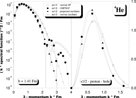
Figure 2: The square of 3–momentum k times the square of the (reduced) spectral function is plotted versus the 3–momentum for the s1/2–proton–hole in the nucleus ⁴He. Open circles refer to the results (7) of normal Hartree–Fock with subtraction of the kinetic energy of the center of mass motion before the variation, full circles to the results (22) of Hartree–Fock with projection into the center of mass rest frame before the variation. For comparison the normal (open inverted triangles) and projected (full triangles) for pure oscillator occupation are presented. In the left part of the figure we display the corresponding curves in a logarithmic, in the right part in a linear scale. The integral over 3–momentum from zero to infinty yields for the “normal” approaches just one, while for the projected calculations the spectroscopic factors out of figure 1 are obtained. The oscillator length was here $b=1.41$ Fm.

We shall now continue the analysis of the various wave functions obtained in ref. ref1. by investigating hole–spectral functions and the corresponding spectroscopic factors. They play an important role in the analysis of e.g., quasi–elastic electron scattering and one–nucleon transfer reactions, where they are often used to draw conclusions on nucleon–nucleon correlations in the considered nuclei. Such conclusions obviously require the precise knowledge on how “uncorrelated” systems do behave. Now, in the investigation ref2. with oscillator determinants it was already demonstrated that the conventional picture of an uncorrelated system has to be modified : instead of the usual spectroscopic factors of one for all the occupied orbits, Galilei–invariance requires a considerable depletion of the spectroscopic factors for hole–states with excitation energies larger or equal to $1\hbar\omega$, while in the last occupied shell an enhancement of the spectroscopic factors is obtained. Consequently, in the analysis of correlations not the usual, but the Galilei–invariance respecting projected spectroscopic factors should be taken as reference. However, in ref. ref2. only simple oscillator configurations were studied, and it is not clear a priori whether the much more realistic Hartree–Fock states produce similar features. This question will be answered in the present paper.

2 Spectral functions and spectroscopic factors.

In the following we shall first summarize the usual definition of hole–spectral functions and spectroscopic factors and then present their Galilei–invariant form. Since we want to evaluate them with the Galilei–invariant Hartree–Fock ground states obtained in ref. ref1. we shall restrict ourselves in the derivation to “uncorrelated” systems, i.e. to one–determinant states of the form

$$|D\rangle\,\equiv\,\prod\limits_{h=1}^{A}\,b_{h}^{\dagger}|0\rangle,$$ (1)

where $|0\rangle$ denotes the particle vacuum. The determinant (1) is composed out of single particle states

$$|h\rangle\,=\,b_{h}^{\dagger}|0\rangle\,=\,\sum\limits_{i=1}^{M_{b}}|i\rangle D_{ih}^{*}\,=\,\sum\limits_{i=1}^{M_{b}}c_{i}^{\dagger}|0\rangle D_{ih}^{*}$$ (2)

which are obtained by a unitary, in general $M_{b}\times M_{b}$–dimensional, transformation $D$ from the $M_{b}$ spherical basis states $|i\rangle\,=\,|\tau_{i}n_{i}l_{i}j_{i}m_{i}\rangle$ defining our model space. The corresponding creation operators will be denoted by $\{c_{i}^{\dagger},\,i=1,...,M_{b}\}$. For these basis states we shall take spin–orbit coupled spherical harmonic oscillator wave functions. As usual $\tau_{i}$ denotes the isospin projection, $n_{i}\,(=0,1,...)$ the node number, $l_{i}$ the orbital angular momentum, which is coupled with the spin to total angular momentum $j_{i}$, and $m_{i}$ is the 3–projection of the latter. We shall furthermore restrict ourselves to transformations (2), which conserve the spherical symmetry of the basis orbits. Then each hole state $|h\rangle$ has definite $\tau_{h}$, $l_{h}$, $j_{h}$ and $m_{h}$ and the transformation (2) does not depend on $m_{h}$. For each set of quantum numbers the sum runs only over the node number $n$ and eq. (2) reduces to

$$|h\rangle\,=\,|\tau_{h}\alpha_{h}l_{h}j_{h}m_{h}\rangle\,=\,\sum\limits_{n}|\tau_{h}nl_{h}j_{h}m_{h}\rangle\,D^{\tau_{h}l_{h}j_{h}}_{n\alpha_{h}},$$ (3)

where we have assumed in addition that the transformation matrix $D$ is purely real. For doubly–even nuclei with closed j–shells the determinant (1) is then spherically symmetric, too, and has total angular momentum and parity $0^{+}$.

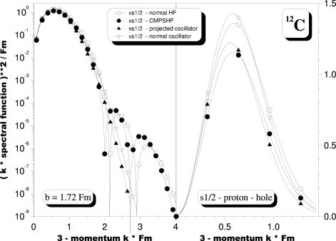
Figure 3: Same as in Fig. 2, but for the s1/2–proton–hole in the nucleus ¹²C. Here the oscillator length was $b=1.72$ Fm.

Furthermore we shall introduce creation operators $C_{\vec{k}\,\tau\sigma}$

$$|\vec{k}\,\tau\sigma\rangle\,\equiv\,C_{\vec{k}\,\tau\sigma}|0\rangle,$$ (4)

which create from the particle vacuum a nucleon in a plane wave state with linear momentum $\hbar\vec{k}$ and spin– and isospin–projections $\sigma$ and $\tau$. As usual, the hole–spectral function is then defined as the probability amplitude to pick out such a plane wave nucleon from a definite hole state $h$

$$f_{h\tau\sigma}^{nor}(\vec{k}\,)\,\equiv\,\langle D|C_{\vec{k}\,\tau\sigma}^{\dagger}b_{h}|D\rangle\,=\,\langle h|\vec{k}\,\tau\sigma\rangle$$ (5)

where the superscript $nor$ indicates that the usual (or “normal”) prescription is used. For all the hole states $h$ occupied in the one–determinant state (1) this expression gives essentially (the complex conjugate of) the Fourier–transform of the corresponding single particle wave function. Evaluation of eq. (5) yields right away

$$f_{h\tau\sigma}^{nor}(\vec{k}\,)\,=\,\delta_{\tau\tau_{h}}\,i^{l_{h}}\,\sum\limits_{\lambda_{h}}\,Y_{l_{h}\lambda_{h}}^{*}(\hat{k})\times$$

$$\times(l_{h}1/2j_{h}|\lambda_{h}\sigma m_{h})\,g_{\tau_{h}\alpha_{h}l_{h}j_{h}}^{nor}(k),$$ (6)

where the “reduced” spectral function $g_{\tau_{h}\alpha_{h}l_{h}j_{h}}^{nor}(k)$ is given by

$$g_{\tau_{h}\alpha_{h}l_{h}j_{h}}^{nor}(k)\,=\,\sum\limits_{n}\,(-)^{n}\,D^{\tau_{h}l_{h}j_{h}}_{n\alpha_{h}}\,R_{nl_{h}}(k)$$ (7)

and

$$R_{nl_{h}}(k)=b^{3/2}\exp\left\{-{1\over 2}(bk)^{2}\right\}{\tilde{R}}_{nl_{h}}(bk)$$

$$=(-)^{n}\sqrt{{2\over{\pi}}}\int\limits_{0}^{\infty}drr^{2}j_{l_{h}}(kr)\,R_{nl_{h}}(r)$$ (8)

is the Fourier–transform of the usual radial harmonic oscillator function $R_{nl_{h}}(r)$.

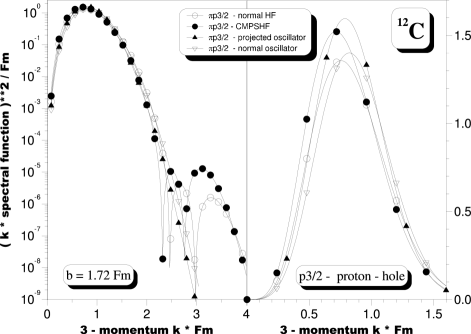
Figure 4: Same as in Fig. 3, but for the p3/2–proton–hole in the nucleus ¹²C.

The “normal” hole–spectroscopic factors are then defined as

$$S_{h}^{nor}=\sum\limits_{\sigma}\int d^{3}\vec{k}\,|f_{h\tau\sigma}^{nor}(\vec{k}\,)|^{2}$$

$$=\delta_{\tau\tau_{h}}\int\limits_{0}^{\infty}dkk^{2}\,{g_{\tau_{h}\alpha_{h}l_{h}j_{h}}^{nor}(k)\,}^{2}\,=\,\delta_{\tau\tau_{h}}.$$ (9)

Since the plane waves (4) form a complete set, it is obvious that the hole–spectroscopic factors fulfill the sum rule

$$\sum\limits_{h}S_{h}^{nor}\,=\,A.$$ (10)

Eqs. (1) to (10) summarize the usual picture of an uncorrelated system : the hole–spectroscopic factors are equal to one for all occupied states and vanish for the unoccupied ones, and the hole–spectral functions are nothing but the wave functions of the occupied single nucleon states in momentum representation.

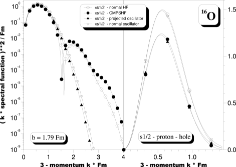
Figure 5: Same as in Fig. 2, but for the s1/2–proton–hole in the nucleus ¹⁶O. Here the oscillator length was $b=1.79$ Fm.

Figure 6: Same as in Fig. 5, but for the p3/2–proton–hole in the nucleus ¹⁶O.

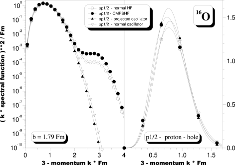
Figure 7: Same as in Fig. 5, but for the p1/2–proton–hole in the nucleus ¹⁶O.

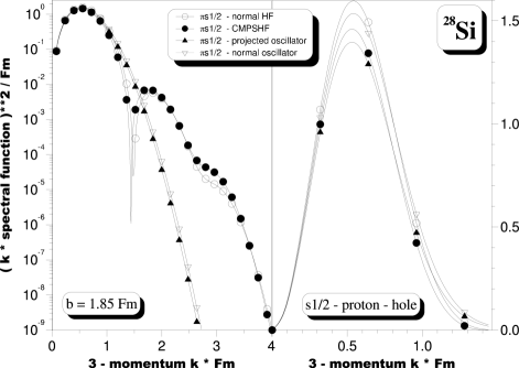
Figure 8: Same as in Fig. 2, but for the s1/2–proton–hole in the nucleus ²⁸Si. Here the oscillator length was $b=1.85$ Fm.

Obviously, the above description is not Galilei–invariant. First of all, neither the ground state $|D\rangle$ of the considered A–nucleon system nor the states $b_{h}|D\rangle$ of the (A-1)–nucleon system live in their respective center of mass rest frame but contain “spurious” admixtures from the motion of the corresponding systems as a whole. In order to obtain a Galilei–invariant description, as demonstrated in ref. ref1. , instead of the determinant (1)

$$|D;\,0\rangle\,\equiv\,{{\hat{C}(0)|D\rangle}\over{\sqrt{\langle D|\hat{C}(0)|D\rangle}}}$$ (11)

has to be used as test wave function in the variational calculation yielding the Hartree–Fock transformation $D$. Here

$$\hat{C}(0)\,\equiv\,\int d^{3}\vec{a}\,\hat{S}(\vec{a}\,)$$ (12)

where

$$\hat{S}(\vec{a}\,)\,\equiv\,\exp\left\{i\vec{a}\cdot\hat{P}\right\}$$ (13)

is the usual shift operator ($\hat{P}$ being the operator of the total linear momentum of the considered system), projects $|D\rangle$ in its center of mass rest frame. For the normalization in eq. (11) we obtain

Figure 9: Same as in Fig. 8, but for the p3/2–proton–hole in the nucleus ²⁸Si.

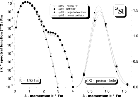
Figure 10: Same as in Fig. 8, but for the p1/2–proton–hole in the nucleus ²⁸Si.

$$N_{0}=\langle D|\hat{C}(0)|D\rangle\,=\,\int d^{3}\vec{a}\,\langle D|\hat{S}(\vec{a}\,)|D\rangle$$ (14)

$$=\,4\pi b^{3}\int\limits_{0}^{\infty}d\alpha\,\alpha^{2}\,\exp\left\{-{A\over 4}\,\alpha^{2}\right\}\,{\rm det}\,s(\alpha)$$

$$=\,4\pi b^{3}\left({4\over A}\right)^{3/2}\,\int\limits_{0}^{\infty}dy\,{\rm e}^{-y^{2}}\,y^{2}\,{\rm det}\,s\left({2\over{\sqrt{A}}}y\right)\,$$

$$=4\pi b^{3}\left({4\over A}\right)^{3/2}\,n_{0}$$ (15)

where $b$ is the oscillator length parameter, $\vec{\alpha}\,\equiv\,\vec{a}/b$, $y=\alpha\sqrt{A}/2$ and the single particle matrix elements of the shift operator

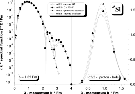
Figure 11: Same as in Fig. 8, but for the d5/2–proton–hole in the nucleus ²⁸Si.

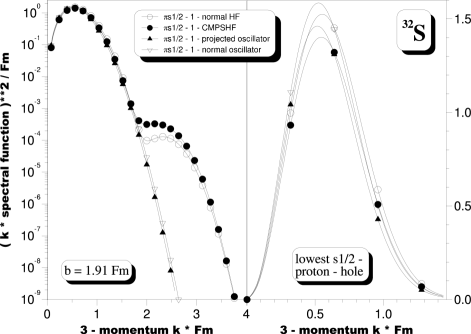
Figure 12: Same as in Fig. 2, but for the lowest s1/2–proton–hole in the nucleus ³²S. Here the oscillator length was $b=1.91$ Fm.

$$s_{hh^{\prime}}(\alpha)\,\equiv\,{\rm e}^{\alpha^{2}/4}\,\langle h|\hat{S}(\hat{e}_{z}\cdot\vec{a}\,)|h^{\prime}\rangle$$ (16)

have been given in ref. ref1. . In eqs. (14) and (16) we have used that $|D\rangle$ is spherically symmetric (i.e., invariant under rotations) so that we can put the shift vector without loss of generality into the z–direction.

Figure 13: ame as in Fig. 12, but for the p3/2–proton–hole in the nucleus ³²S.

Figure 14: Same as in Fig. 12, but for the p1/2–proton–hole in the nucleus ³²S.

In the same way we define

$$N_{hh^{\prime}}\,\equiv\,\langle D|b^{\dagger}_{h}\hat{C}(0)b_{h^{\prime}}|D\rangle\,\equiv\,4\pi b^{3}\left({4\over{A-1}}\right)^{3/2}\,n_{hh^{\prime}}$$

and

$$H_{hh^{\prime}}\,\equiv\,\langle D|b^{\dagger}_{h}\hat{H}\hat{C}(0)b_{h^{\prime}}|D\rangle\,\equiv\,4\pi b^{3}\left({4\over{A-1}}\right)^{3/2}\,h_{hh^{\prime}}$$

where $\hat{H}$ denotes the same Hamiltonian as has been used to obtain the Hartree–Fock transformation $D$. Solving the generalized eigenvalue problem

$$(h-En)w\,=\,0\qquad{\rm with}\qquad w^{T}nw\,\equiv\,{\bf 1}$$ (19)

the Galilei–invariant form of the one–hole states can be written as

$$|\tilde{h};\,0\rangle\,=\,{\sum\limits_{\alpha_{h}}}^{(\tau_{h}l_{h}j_{h})}\hat{C}(0)b_{h}|D\rangle\,w^{\tau_{h}l_{h}j_{h}}_{\alpha_{h}\tilde{h}}\,{1\over{\sqrt{4\pi b^{3}(4/(A-1))^{3/2}}}}$$

Furthermore, for the outgoing (or incoming) continuum nucleon not the state (4) but a relative wave function with respect to the (A-1)–nucleon system should be used. Consequently, we get for the Galilei–invariant hole–spectral function

$$f_{\tilde{h}\tau\sigma}^{proj}(\vec{k}\,)=\delta_{\tau\tau_{h}}\,{{n_{0}^{-1/2}}\over{4\pi b^{3}(4/A)^{3/4}(4/(A-1))^{3/4}}}\times$$

$$\times{\sum\limits_{\alpha_{h}}}^{(\tau_{h}l_{h}j_{h})}\langle D|C^{\dagger}_{\vec{k}\,\tau\sigma}\exp\{-i\vec{k}\cdot\vec{R}_{A-1}\}\hat{C}(0)b_{h}|D\rangle\ w^{\tau_{h}l_{h}j_{h}}_{\alpha_{h}\tilde{h}}$$

$$=\delta_{\tau\tau_{h}}\,{{n_{0}^{-1/2}}\over{4\pi b^{3}(4/A)^{3/4}(4/(A-1))^{3/4}}}{\sum\limits_{\alpha_{h}}}^{(\tau_{h}l_{h}j_{h})}{\sum\limits_{\alpha_{h^{\prime}}l_{h^{\prime}}j_{h^{\prime}}m_{h^{\prime}}}}^{(\tau_{h})}$$

$$\langle h^{\prime}|\vec{k}\,\tau_{h}\sigma\rangle\langle D|b^{\dagger}_{h^{\prime}}\exp\{-i\vec{k}\cdot\vec{R}_{A-1}\}\hat{C}(0)b_{h}|D\rangle\,w^{\tau_{h}l_{h}j_{h}}_{\alpha_{h}\tilde{h}}$$

where $\vec{R}_{A-1}$ denotes the center of mass coordinate of the (A-1)–nucleon system. Again the spherical symmetry of $|D\rangle$ and the properties of the hole–creation and –annihilation operators under rotations can be used to put for the evaluation of the matrix element in eq. (2) one vector without loss of generality in the z–direction. Here we choose $\vec{k}\,=\,\hat{e}_{z}\cdot\vec{k}$. In analogy to eq. (2) we can write

$$f_{\tilde{h}\tau\sigma}^{proj}(\vec{k}\,)\,=\,\delta_{\tau\tau_{h}}\,i^{l_{h}}\,\sum\limits_{\lambda_{h}}\,Y_{l_{h}\lambda_{h}}^{*}(\hat{k})(l_{h}1/2j_{h}|\lambda_{h}\sigma m_{h})\,g_{\tau_{h}\tilde{h}\,l_{h}j_{h}}^{proj}(k)$$

where the “reduced” projected spectral function is now given by

$$g_{\tau_{h}\tilde{h}\,l_{h}j_{h}}^{proj}(k)=\left({A\over{A-1}}\,b^{2}\right)^{3/4}\exp\left\{-{1\over 2}{A\over{A-1}}(bk)^{2}\right\}n_{0}^{-1/2}$$

$${\sum\limits_{\alpha_{h}}}^{(\tau_{h}l_{h}j_{h})}w^{\tau_{h}l_{h}j_{h}}_{\alpha_{h}\tilde{h}}{\sum\limits_{l_{h^{\prime}}j_{h^{\prime}}\alpha_{h^{\prime}}}}^{(\tau_{h})}\tilde{R}^{\tau_{h}l_{h^{\prime}}j_{h^{\prime}}}_{\alpha_{h^{\prime}}}(bk)$$

$$\sum\limits_{L}\Delta(l_{h},\,l_{h^{\prime}},\,L){1\over 2}\left[1+(-)^{l_{h}+l_{h^{\prime}}+L}\right]\sqrt{{{2j_{h^{\prime}}+1}\over{2j_{h}+1}}}$$

$$(-)^{j_{h^{\prime}}-1/2}(j_{h^{\prime}}j_{h}L|1/2-1/20)2$$

$$\sum\limits_{m>0}(-)^{j_{h}-m}(j_{h^{\prime}}j_{h}L|m-m0)$$

$$exp\left\{{1\over{A-1}}\left({{bk}\over 2}\right)^{2}\right\}\int\limits_{0}^{\infty}dy{\rm e}^{-y^{2}}y^{2}\int\limits_{0}^{\pi/2}d\vartheta\sin\vartheta$$

$$\Biggl{\{}{1\over 2}[1+(-)^{l_{h}+l_{h^{\prime}}}](-)^{(l_{h^{\prime}}-l_{h})/2}\times$$

$${\rm Re}\Biggl{[}\left(z^{(\tau_{h})}(bk,\alpha,\vartheta)\right)^{-1}_{\alpha_{h}l_{h}j_{h}m;\,\alpha_{h^{\prime}}l_{h^{\prime}}j_{h^{\prime}}m}\,{\rm det}\,z\Biggr{]}+$$

$$+\,{1\over 2}[1-(-)^{l_{h}+l_{h^{\prime}}}](-)^{(l_{h^{\prime}}-l_{h}-1)/2}\times$$

$${\rm Im}\Biggl{[}\left(z^{(\tau_{h})}(bk,\alpha,\vartheta)\right)^{-1}_{\alpha_{h}l_{h}j_{h}m;\,\alpha_{h^{\prime}}l_{h^{\prime}}j_{h^{\prime}}m}\,{\rm det}\,z\Biggr{]}\Biggr{\}}$$

Here $\Delta(l_{h},\,l_{h^{\prime}},\,L)=1$ if $|l_{h}-l_{h^{\prime}}|\leq L\leq l_{h}+l_{h^{\prime}}$ and $=0$ if not, $y\,\equiv\,\alpha\sqrt{A-1}/2$, $\vartheta$ is the angle between the shift vector and the z–direction and

$$\tilde{R}^{\tau_{h}l_{h^{\prime}}j_{h^{\prime}}}_{\alpha_{h^{\prime}}}(bk)\,\equiv\,\sum\limits_{n^{\prime}}\,(-)^{n^{\prime}}\,D^{\tau_{h}l_{h^{\prime}}j_{h^{\prime}}}_{n^{\prime}\alpha_{h^{\prime}}}\,\tilde{R}_{n^{\prime}l_{h^{\prime}}}(bk)\noindent$$ (24)

denotes the polynomial part of the Fourier–transform of the radial wave function of the hole state $h^{\prime}$. The matrix elements of $z^{(\tau_{h})}$ are identical to those given in appendix B of ref. ref1. except for the fact that the argument $qb/A$ has to be replaced here by $kb/(A-1)$. The determinant factorizes in a proton– and a neutron–part

$${\rm det}z\,=\,\prod\limits_{\tau=p,n}\,{\rm det}z^{(\tau)}$$ (25)

and obviously depends on the same arguments as the matrix elements of the inverse matrices $(z^{(\tau)})^{-1}$ in eq. (2).

Figure 15: Same as in Fig. 12, but for the d5/2–proton–hole in the nucleus ³²S.

Similarly as in eq. (2), the projected spectroscopic factors are then defined by

$$S_{\tilde{h}}^{proj}\,\equiv\,\sum\limits_{\sigma}\int d^{3}\vec{k}\,|f_{\tilde{h}\tau\sigma}^{proj}(\vec{k}\,)|^{2}\,$$

$$=\delta_{\tau\tau_{h}}\int\limits_{0}^{\infty}dk\,k^{2}\,{g_{\tau_{h}\tilde{h}\,l_{h}j_{h}}^{proj}(k)\,}^{2}$$ (26)

It has been demonstrated in ref. ref2. that, if the hole states (2) are pure harmonic oscillator states and if $|D\rangle$ is a “non–spurious” oscillator determinant, then eqs. (2) and (2) can be evaluated analytically. In this case one does not even have to solve the generalized eigenvalue problem (19). In all doubly closed j–shell nuclei up to ²⁸Si, the overlap matrix $n_{hh^{\prime}}$ out of eq. (2) is diagonal, so that the $w$’s needed in eq. (2) are simply the inverse square roots of its diagonal elements. In ³²S and ⁴⁰Ca two s–states are occupied and do mix via eq. (2). Here one can always Gram–Schmidt–orthonormalize the 0s–state with respect to the 1s–state as has been shown in ref. ref2. . The result of these analytical calculations was that the (reduced) hole spectral function (2) can be written as

$$g_{\tau_{h}\tilde{h}\,l_{h}j_{h}}^{proj;\,osc}(k)\,\equiv\,R^{rel}_{\tilde{h}l_{h}}(k)\,\sqrt{S^{proj;\,osc}_{\tilde{h}}}$$ (27)

where, in the one–dimensional cases, the subscript $\tilde{h}\,=\,n_{h}$ and

$$R^{rel}_{n_{h}l_{h}}(k)=(-)^{n_{h}}\left({A\over{A-1}}\,b^{2}\right)^{3/4}$$

$$\exp\left\{-{1\over 2}{A\over{A-1}}(bk)^{2}\right\}\,\tilde{R}_{n_{h}l_{h}}\left(\sqrt{{A\over{A-1}}}bk\right),$$ (28)

while for the lowest s–states in ³²S and ⁴⁰Ca the $R^{rel}_{\tilde{h}l_{h}}$ are linear combinations of the functions (2) for $l_{h}=0$ and $n_{h}=0,\,1$ with the corresponding expansion coefficients resulting from the orthonormalization. The functions (2) are just the usual oscillator wave functions in momentum representation, however, the nucleon mass $M$ entering the parameter $b$ has been replaced by the reduced mass $(A-1)M/A$. This is indicated by the superscript $rel$. The analytical evaluation in ref. ref2. yielded

$$S^{proj;\,osc}_{\tilde{h}}\,=\,\left\{\matrix{1&{\rm for}\;0s-{\rm holes}\;{\rm in}\;^{4}{\rm He}\cr&\cr{4\over 5}&{\rm for}\;0s-{\rm holes}\;{\rm in}\;^{16}{\rm O}\cr&\cr{{16}\over{15}}&{\rm for}\;0p-{\rm holes}\;{\rm in}\;^{16}{\rm O}\cr&\cr{{1410}\over{1521}}&{\rm for}\;0\tilde{s}-{\rm holes}\;{\rm in}\;^{40}{\rm Ca}\cr&\cr{{1400}\over{1521}}&{\rm for}\;0p-{\rm holes}\;{\rm in}\;^{40}{\rm Ca}\cr&\cr{{1600}\over{1521}}&{\rm for}\;1s-{\rm holes}\;{\rm in}\;^{40}{\rm Ca}\cr&\cr{{1600}\over{1521}}&{\rm for}\;0d-{\rm holes}\;{\rm in}\;^{40}{\rm Ca}\cr}\right\}$$ (29)

It is easily checked that

$$\sum\limits_{\tilde{h}}\,S^{proj;\,osc}_{\tilde{h}}\,=\,A$$ (30)

as expected, since the functions (27) form again a complete orthonormal set. On first sight it may seem strange to obtain spectroscopic factors which are larger than one, however, the oscillator results (28) are identical to those obtained by Dieperink and de Forest ref10. with rather different methods and are easy to understand by simple considerations as discussed in ref. ref2. .

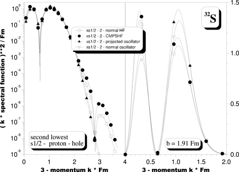
Figure 16: Same as in Fig. 12, but for the second lowest s1/2–proton–hole in the nucleus ³²S.

Unlike the “normal” result (7) and the projected oscillator result (27) for non–spurious oscillator determinants $|D\rangle$, the general form of the reduced spectral function (2) cannot be written as the product of a normalized single particle wave function times some number. Thus the sum of the spectroscopic factors over all hole–states does in general yield a smaller number than A, since $\exp\{-i\vec{k}\cdot\vec{R}_{A-1}\}C_{\vec{k}\,\tau\sigma}|D\rangle$ does not contain the complete set of configurations created by $\hat{C}(0)\,b_{h}|D\rangle$. We therefore write

$$\sum\limits_{\tilde{h}}\,S^{proj}_{\tilde{h}}\,=\,A\,-\,\epsilon$$ (31)

It turns out, however, that for the cases discussed in the next section $\epsilon/A$ varies only between 0.12 and 0.35 percent. The violation of the sum rule due to non–trivial correlations induced by the projector into the uncorrelated Hartree–Fock systems investigated here is hence rather small, and at least approximately, the separation of eq. (2) into a product of a normalized single particle function and the square root of the spectroscopic factor is still true.

3 Results and discussion.

We considered here the six doubly closed j–shell nuclei ⁴He, ¹²C, ¹⁶O, ²⁸Si, ³²S and ⁴⁰Ca. In ref. ref1. for these nuclei the results of Galilei–invariant spherical Hartree–Fock calculations with projection into the center of mass rest frame have been compared to those of standard spherical Hartree–Fock calculations, in which only the kinetic energy of the center of mass motion was subtracted from the hamiltonian before the variation. As hamiltonian the kinetic energy plus the Coulomb interaction plus the Brink–Boeker force B1 [6] complemented with a short range (0.5 Fm) two–body spin–orbit term having the same volume integral as the Gogny–force D1S ref7. has been used. The Hartree–Fock wave functions resulting from these calculations using as single particle basis 19 major oscillator shells will be analyzed in the following. Furthermore, as in ref. ref1. , also here the results will be compared to those obtained with simple oscillator determinants.

We shall first discuss the hole–spectroscopic factors. Since in the normal approach these are all equal to one (see eq. (2)), irrespective whether one uses simple oscillator determinants or the Hartree–Fock ground states $|D_{c}\rangle$ out of eq. (2) in ref. ref1. , we can restrict ourselves to the discussion of the Galilei–invariant spectroscopic factors out of eqs. (27) and (2) for the oscillator occupations and for the Hartree–Fock ground states $|D_{pr}\rangle$ (see eq. (29) of ref. ref1. ) obtained with projection into the center of mass rest frame before the variation, respectively. Since furthermore in the oscillator approach proton– and neutron–hole–spectroscopic factors are identical and even in the Hartree–Fock approach almost undistiguishable, only the proton–hole spectroscopic factors will be discussed.

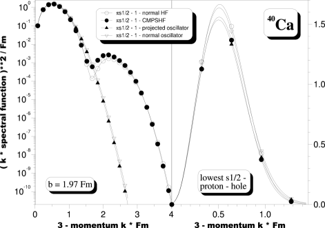
Figure 17: Same as in Fig. 2, but for the lowest s1/2–proton–hole in the nucleus ⁴⁰Ca. Here the oscillator length was $b=1.97$ Fm.

Figure 18: Same as in Fig. 17, but for the p3/2–proton–hole in the nucleus ⁴⁰Ca.

The results are summarized in figure 1. Open symbols refer to the projected oscillator, closed (or crossed) symbols to the projected Hartree–Fock results. On the abscissa the relevant orbits are presented. They are pure oscillator orbits (or for the 0s1/2–states in ³²S and ⁴⁰Ca the states resulting from Gram–Schmidt orthonormalization with respect to the 1s1/2–states) in the former, the lowest (“0”) or second lowest (“1”) Hartree–Fock single particle states resulting from the solution of eq. (18) for each set of $l$ and $j$ quantum numbers in the latter case. The figure clearly shows that, though based on rather different wave functions, oscillator and Hartree–Fock results are almost identical. Thus for the spectroscopic factors, which are integral properties, the choice of the single particle basis, which is irrelevant in the normal approach, does not seem to matter in the Galilei–invariant prescription either, at least as long as only uncorrelated systems are considered. As already discussed in ref. ref2. , one sees a considerable depletion of the strengths of the hole–states with excitation energies larger or equal to $1\hbar\omega$ and an enhancement of the strengths of the hole–orbits near the Fermi–energy. The depletion of the lowest s–state in ¹⁶O is as large as 20 percent and even for the lowest s– and p3/2–states in ³²S and ⁴⁰Ca still depletions of more than 8 percent are obtained. Exceptions of the $\hbar\omega$–rule are the spectroscopic factors of the p1/2–holes in ²⁸Si and ³²S. Though belonging to the second but last shell below the Fermi–energy, these are considerably less affected by the projection than their p3/2–spin–orbit partners. A similar spin–orbit effect for these orbits was also seen in the corresponding single particle energies discussed in ref. [1]. It results from the presence of the d5/2 and the absence of the d3/2–orbit in both these nuclei and indicates the dominance of couplings to angular momentum one in the spurious center of mass motion.

As already discussed, the oscillator results fulfill the sum rule (29) exactly, while for the Hartree–Fock this is only approximately true (see eq. (31)). However, from the fact that oscillator and Hartree–Fock spectroscopic factors are almost identical, it is clear that the violation $\epsilon$ of the sum rule (31) is, as mentioned before, only a rather small effect. It was furthermore discussed in ref. ref4. that in the oscillator approach both the normal spectroscopic factors (all equal to one) together with the normal single particle energies as well as the projected spectroscopic factors together with the projected single particle energies fulfill Kolthun’s sum rule ref11. exactly, which was interpreted as a nice check for the consistency of the projected results. Now, in case of the harmonic oscillator approach, the projected total energy for the A–nucleon ground state is identical to that of the normal approach, provided the latter is corrected by subtracting the kinetic energy of the center of mass motion. As has been demonstrated in ref. ref1. , in the Hartree–Fock prescription this is not the case. Thus, while in the normal Hartree–Fock approach Kolthun’s sum rule is fulfilled by definition, in the projected Hartree–Fock prescription, as already for the total hole–strength sum rule (31), this is only approximately true. However, again the violation is small.

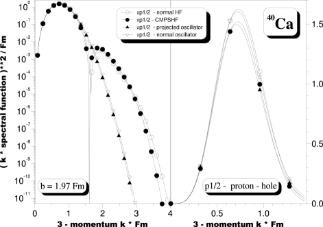
Figure 19: Same as in Fig. 17, but for the p1/2–proton–hole in the nucleus ⁴⁰Ca.

Figure 20: Same as in Fig. 17, but for the d5/2–proton–hole in the nucleus ⁴⁰Ca.

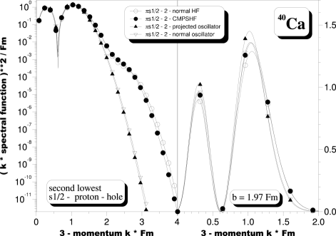
Figure 21: Same as in Fig. 17, but for the second lowest s1/2–proton–hole in the nucleus ⁴⁰Ca.

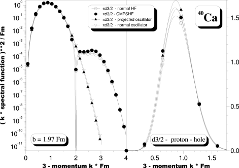
Figure 22: Same as in Fig. 17, but for the d3/2–proton–hole in the nucleus ⁴⁰Ca.

The results presented in figure 1 show that our usual picture of an uncorrelated system has to be changed considerably. This has important consequences for the analysis of experiments, in which deviations of the hole spectroscopic factors from one are usually interpreted as fingerprints of nucleon–nucleon correlations. However, we have shown that in a Galilei–invariant description the spectroscopic factors even of an uncorrelated system differ from one considerably. Only deviations from the projected results out of figure 1 can be related to non–trivial correlations.

We shall now turn our attention to the reduced spectral functions. Again only the results for the proton–hole states will be presented. The results for the different proton–hole states in the various considered nuclei are presented in figures 2 to 22. The figures show the square of the reduced spectral functions times the square of the 3–momentum as functions of the 3–momentum. In the left part of each figure the results are given in a logarithmic, in the right part in a linear scale. Open circles refer to the normal results (eq. (7)) for the ground states obtained with standard spherical Hartree–Fock subtracting the kinetic energy of the center of mass motion from the Hamiltonian before the variation in ref. ref1. . The integrals over 3–momentum from zero to infinity yield for these curves always one. Closed circles denote the results (eq. (2)) for the ground states obtained by Galilei–invariant projected Hartree–Fock calculations (CMPSHF) in ref. ref1. . Here the integral yields the projected spectroscopic factors out of eq. (25), which are displayed by full (or crossed) symbols in figure 1. Open inverted triangles represent again the results (7) of the normal approach, however, now for simple oscillator ground states. The integrals of these functions are obviously again all equal to one. Finally, full triangles are used for the (analytically obtained) projected oscillator results. Here the integrals yield the harmonic oscillator spectroscopic factors out of eq. (27), which are displayed by open symbols in figure 1.

Figure 2 displays the reduced proton spectral functions for s1/2–proton–holes in ⁴He. Here oscillator and Hartree–Fock results are rather similar at low momenta (below about 2 inverse Fm), while at higher momenta they differ considerably due to the major shell mixing in the latter. On the other hand the projected results for both approaches differ considerably from the unprojected ones already at low momenta. Since (see figure 1) the integrals of all curves give almost the same spectroscopic factor one, this large difference is entirely due to the fact that the projected approaches yield relative wave functions instead of the usual ones. The difference between relative and usual wave functions is obviously largest in ⁴He and decreases with increasing mass number.

Figure 3 shows the same plots for the s1/2–proton–holes in ¹²C. Again a rather large similarity between oscillator and Hartree–Fock results is obtained at low momenta, while large differences are seen above about 2 inverse Fm. Because of the larger mass, the difference of relative and usual wave functions is here less pronounced, however, now the projected results are quenched by about 18 percent with respect to the normal ones due to the considerably smaller spectroscopic factor.

For the p3/2–proton–holes in ¹²C in figure 4, the difference of oscillator and Hartree–Fock results due to the larger major shell mixing increases already at low momenta. Instead of a quenching, because of the larger spectroscopic factor here an enhancement of the projected results with respect to the unprojected ones is seen.

The results for the various proton–hole states in ¹⁶O displayed in figures 5 to 7 show, as expected, rather similar features as those for ¹²C, except that here the major shell mixing becomes even more important, so that the deviations of the Hartree–Fock results from the oscillator ones are larger and start already at lower momenta. Again, according to the corresponding spectroscopic factors, the projected s1/2–spectral functions (figure 5) are quenched with respect to the usual ones, while for the projected p3/2– (figure 6) and p1/2–spectral functions (figure 7) an enhancement is obtained.

Similar arguments hold for the various hole states in ²⁸Si (figures 8 to 11). Here the projected spectral functions for the s1/2– (figure 8) and p3/2–holes (figure 9) are quenched, while those for the d5/2–holes (figure 11) show an enhancement due to the corresponding spectroscopic factors. That such an (though small) enhancement is also seen for the projected p1/2–hole–spectral functions (figure 10) is due to the absence of the d3/2–state in the ground state and has been discussed already above.

This pattern is essentially repeated for ³²S (figures 12 to 16). The projected spectral functions are quenched for the lowest s1/2– (figure 12) and the p3/2–states (figure 13), enhanced for the d5/2– (figure 15) and second lowest s1/2–states (figure 16), while for the p1/2–state (figure 14) though belonging to the second but last occupied shell because of the occupied d5/2– and unoccupied d3/2–orbits again a slight enhancement is obtained.

Finally, for the doubly closed shell nucleus ⁴⁰Ca (figures 17 to 22) the spectral functions out of the last occupied shell (d5/2, second lowest s1/2 and d3/2 in figures 20, 21 and 22, respectively) are enhanced by almost the same factor, while for the holes with excitation energy $1\hbar\omega$ (p3/2 and p1/2 in figures 18 and 19) or $2\hbar\omega$ (the lowest s1/2 in figure 17) the projected results are quenched with respect to the normal ones.

Note, that in all cases, though sometimes a little obscured by the logarithmic plotting, considerable differences are seen between the projected and the normal Hartree–Fock hole–spectroscopic functions, which can not be explained by “quenching” or “enhancement” due to the corresponding spectroscopic factors alone. This demonstrates that the single particle wave functions obtained by the Galilei–invariant Hartree–Fock prescription are rather different from those obtained via the usual Hartree–Fock approach as it has been demonstrated already by other observables in ref. ref1. .

4 Conclusions.

Normally, we describe the ground state of an uncorrelated A–nucleon system by a single Slater–determinant, in which the energetically lowest A single particle states are fully occupied while the higher orbits are empty. The hole–spectral functions of such a system are then the Fourier–transforms of the single particle states it is composed of, and the hole–spectroscopic factors are all equal to one.

This simple picture, however, is not true any more, if Galilei–invariance is respected. As already demonstrated in ref. [10,2] using simple oscillator configurations for the ground state of some doubly–closed major shell nuclei, Galilei–invariance requires a considerable depletion of the spectroscopic factors for hole–states out of the second and third but last shell below the Fermi–energy, while those for the hole–states out of the last shell are enhanced, so that the sum rule for the total hole–strength remains conserved.

These results are nicely confirmed even for the more realistic Hartree–Fock wave functions analyzed in the present paper. The Galilei–invariance respecting hole–spectroscopic factors for the Hartree–Fock ground states resulting from calculations with projection into the center of mass rest frame before the variation are almost identical to the projected oscillator results from ref. [2] and thus fulfill the sum rule for the total hole–strength in a very good approximation, too. Furthermore, in both the oscillator as well as the Hartree–Fock description, Galilei–invariance induces an interesting spin–orbit effect into the 0p–shell of the closed subshell nuclei ²⁸Si and ³²S. On the other hand, as expected because of the major shell mixing, the hole spectral functions obtained in the projected Hartree-Fock prescription, are quite different from the simple projected oscillator ones.

The results clearly show, that not only in the simple oscillator approximation but also for more realistic approaches the simple picture of an uncorrelated system has to be changed considerably if Galilei-invariance is respected. This may have serious consequences for the analysis of correlations in the nuclei, since the correct uncorrelated reference is considerably different from that which is usually assumed.

- (1) R.R. Rodríguez-Guzmán, K.W. Schmid, Eur. Phys. J. A 19, 45 (2004). (see also arXiv:nucl-th/0503059)
- (2) K.W. Schmid, Eur. Phys. J. A 12, 29 (2001).
- (3) K.W. Schmid, Eur. Phys. J. A 13, 319 (2002).
- (4) K.W. Schmid, Eur. Phys. J. A 14, 413 (2002).
- (5) K.W. Schmid, Eur. Phys. J. A 16, (2003), in press.
- (6) D.M. Brink, E. Boeker, Nucl. Phys. A 91, 1 (1966).
- (7) J.F. Berger, M. Girod, D. Gogny, Comp. Phys. Commun. 63, 365 (1991).
- (8) L.J. Tassie, C.F. Barker, Phys. Rev. 111, 940 (1958).
- (9) K.W. Schmid, P.–G. Reinhard, Nucl. Phys. A 530, 283 (1991).
- (10) A.E.L. Dieperink, T. de Forest, Phys. Rev. C 10, 543 (1974).
- (11) D.J. Thouless, Nucl. Phys. 21, 225 (1960).